The Overall Efficiency in the Presence of Imprecise Adaptable Measures

Available online at http://ijdea.srbiau.ac.ir

Int. J. Data Envelopment Analysis (ISSN 2345-458X)

Vol.4, No.4, Year 2016 Article ID IJDEA-00422, 10 pages Research Article

The Overall Efficiency in the Presence of

Imprecise Adaptable Measures

Sohrab Kordrostami

a

, Monireh Jahani Sayyad Noveiri

b *

(a)

Department of Mathematics, Lahijan Branch, Islamic Azad University, Lahijan,

Iran

(b)

Young

Researchers and Elite

Club,

Lahijan Branch

, Islamic Azad

University,

Lahijan,

Iran

Received June 27, 2016, Accepted September 28, 2106

Abstract

Traditional data envelopment analysis (DEA) models usually evaluate the efficiency scores of decision making units (DMUs) with precise data from an optimistic point of view where the status of each measure (i.e. input/output) is certain. However, there are occasions in real world applications that measures can play both input and output roles in an imprecise environment. In the current study, measures with two roles, input and output, are called “adaptable measures”. This paper proposes a DEA-based approach for estimating the performance of DMUs where adaptable and fuzzy data exist. Indeed, efficiency scores are calculated from two aspects, optimistic and pessimistic, when there are adaptable and fuzzy data. Two different efficiency scores are integrated into a geometric average efficiency. Thus, the overall efficiency is calculated and adaptable variables are split into input and output variables in evaluating the efficiency of each DMU. A numerical example is used to illustrate the approach.

Keywords: Data envelopment analysis (DEA), Efficiency, Fuzzy data, Adaptable variable.

*. Corresponding author, E-Mail: [email protected]

1. Introduction

Data envelopment analysis (DEA), initially suggested by Charnes et al. [1], is a nonparametric technique to evaluate the relative efficiency of decision making units (DMUs) that use multiple inputs to produce multiple outputs. In conventional DEA models, the efficiency scores of DMUs with crisp inputs/outputs are usually calculated from an optimistic point of view. Wang et al. [2] measured the performance of DMUs with precise data from different points of view, optimistic and pessimistic, and calculated the overall efficiency by using the geometric average efficiency. However, in the real world, there are situations that imprecise data exist. In the DEA literature, there are methods for assessing the efficiency of firms in the presence of vague inputs and outputs.

One of the popular approaches for the efficiency evaluation in the presence of imprecise information is fuzzy DEA methods. Firstly, Sengupta [3] suggested a fuzzy DEA model to incorporate fuzzy data via the tolerance levels definition. Afterwards, various DEA-based approaches are introduced to measure the performance of DMUs with fuzzy factors. Hatami-Marbini et al. [4] reviewed the fuzzy data envelopment analysis literature over 20 years. Also, Emrouznejad and Tavana [5] classified the application of fuzzy set theory in DEA into six groups: the tolerance approach [3, 6], the possibility approach [7, 8], the



-level based approach [9, 10], the fuzzy arithmetic [11, 12] the fuzzy ranking approach [13], and the fuzzy random/type-2 fuzzy set [14, 15]. Readers can refer to Hatami-Marbini et al. [4] and Emrouznejad & Tavana [5] for more information.

Furthermore, the input/output status of measures has been usually specified in the conventional DEA models. Nonetheless, sometimes the input/output status of a variable is uncertain. It means a variable can be considered as both an input and output. In this study, variables with uncertain status are defined as adaptable

have some drawbacks. Firstly, they calculate the efficiency from an optimistic viewpoint. Secondly, the majority of them consider precise inputs and outputs. Finally, the role of a variable is determined as an input or an output.

To tackle the aforementioned drawbacks, in the current paper, the overall efficiency of DMUs is calculated where adaptable and fuzzy data present. Actually, the fuzzy expected value models are introduced to estimate the optimistic and pessimistic efficiencies of DMUs. Then, the efficiency scores are integrated as a geometric average efficiency. Moreover, it is indicated how much of adaptable variable is considered as input and how much as output. In sum, fuzzy expected value DEA models are introduced to specify the efficiency of DMUs where fuzzy adaptable measures exist.

The paper is organized as follows. Section 2 reviews some basic concepts of fuzzy variables, the fuzzy expected value and dual-role factors. In Section 3, a DEA-based methodology is developed that is designed to handle situations that adaptable and fuzzy factors present. A numerical example illustrates and clarifies the proposed approach in Section 4. Conclusions appear in Section 5.

2. Basic concepts and fundamentals

Firstly, basic concepts of fuzzy numbers and related issues are provided in this section. It is pointed out that adaptable measures, which are under consideration in this study, have the similar definition of dual-role factors. Actually, a dual-role factor can play both roles, input and output, simultaneously. So, dual-role factors are also described briefly.

2.1. Fuzzy variables

Definition 2.1. A fuzzy set Ain X is characterized by a membership function

( )

A

x



which associates with each point in

X a real number in the interval

[0,1]

.

( )

A

x



indicates the degree of membership of

x

in A.[29]

Definition 2.2. A fuzzy subset Bof the real numbers R is convex if and only if for

, , [0 ,1]

x y R 

    ,

( (1 ) ) min( ( ), ( ))

B x y B x B y

       .

Definition 2.3. Fuzzy numbers are convex normalized fuzzy set of real numbers in which



( )

x

is piecewise continuous. In this study trapezoidal and triangular fuzzy variables are utilized because of the wide applications of them in practical problems. A trapezoidal fuzzy variable

( , , , )

a b c d





is a fuzzy variable with the following membership function

( ) / ( ) ,

1 ,

( )

( ) / ( ) ,

0 .

x a b a i f a x b

i f b x c x

x d c d i f c x d

o t h e r w i s e

 

   



 _{ }

  

   

  

A triangular fuzzy variable





( , , )

a b c

is a fuzzy variable with a membership function



_ as follows:

( ) / ( ) ,

( ) ( ) / ( ) ,

0 .

x a b a i f a x b

x x c b c i f b x c

o th e r w i s e

 

   

 

 _    

 

Definition 2.4. [30] The expected value of a trapezoidal fuzzy variable





( , , , )

a b c d

is defined as

( )

( )

4

a b c d

E     

Also, the expected value of a triangular fuzzy number





( , , )

a b c

is shown by

( 2 )

( )

4

a b c

E     .

Proposition 1. [30, 31] Assume

f

and g

are fuzzy variables and

a

and

b

are real numbers. Thus, we have

( ) ( ) ( ).

E af bg aE f bE g

2.3. Dual-role factors

and an output, simultaneously. In the literature, these factors are so-called flexible measures and dual-role factors. Factors like trainees in organizations, awards to scholars, and outages in power plants are deemed as dual-role factors. For instance, according to Cook et al. [27] “the number of nurse trainees on staff in a study of hospital efficiency constitutes an output measure for a hospital, but at the same time it is an important component of the hospital’s total staff component, hence it is an input”.

3. Efficiency measurement of DMUs

with fuzzy adaptable variables

In this section, an approach based on DEA is introduced to estimate the overall efficiency of DMUs when fuzzy adaptable variables exist. For this purpose, the efficiency scores of DMUs are firstly calculated from two aspects, optimistic and pessimistic viewpoints.

Assume, there are n DMUs, DMU_j,

(j1,..., )n with m _inputs xij (i1,..., )m ,

s outputs y_rj (r 1,..., )s and k adaptable variables z_tj (t1,..., )k . In this case, inputs, outputs and adaptable variables are considered as trapezoidal fuzzy data, i.e.

( L, M, N, U) ij ij ij ij ij

x  x x x x , y_rj(y_rjL,y_rjM,y_rjN,y_rjU) and

z



_tj ( ,z z_tjL _tjM,z_tjN,z_tjU), respectively. According to Liu and Liu [30] and definition 2.4, we have

( _ij

)

(1/ 4)( _ijL _ijM _ijN _ijU)

E x  x x x x ,

( _rj

)

(1/ 4)( _rjL _rjM _rjN U_rj)

E y  y y y y , and

( _tj

)

(1 / 4)( _tjL _tjM _tjN _tjU)

E z  z z z z .

With considering the continuous variable

t

d

0



d

_t



1

, we define the relative

efficiency of DMU_o , the unit under evaluation, as follows:

1 1

1 1

( )

( (1 ) )

s k

r ro t t to

O p t r t

o m k

i io t t to

i t

E u y w d z e

E v x w d z

 

 

 

 









 

 

(1)

Thatv u_i, _r,andw_tare weights of input, output and adaptable variables, respectively. Also, d_t is used to determine

the portion of adaptable variablez_tj that is

taken as output. Due to proposition 1,e_oOpt

can be rewritten as follows:

1 1

1 1

( ) ( )

( ) (1 ) ( )

s k

r ro t t to

Opt r t

o m k

i io t t to

i t

u E y w d E z e

v E x w d E z

 

 

 

 









 

 

(2)

Thus, the following fractional nonlinear programming is proposed for evaluating the efficiency of

DMU

_ofrom optimistic point of view:

1 1

1 1

1 1

1 1

( ) ( )

( ) (1 ) ( )

( ) ( )

. . 1, 1,..., ,

( ) (1 ) ( )

, , , , , ,

0 1, .

s k

r ro t t to

best r t

o m k

i io t t to

i t

s k

r rj t t tj

r t

m k

i ij t t tj

i t

i r t t

u E y w d E z Max e

v E x w d E z

u E y w d E z

s t j n

v E x w d E z

v u w i r t d t



 

 

 

 

 

 



 

 

 

  

















 

 

 

 

(3)

That



is the non-Archimedean infinitesimal.

( ) 1 ( ) 1 ( ) 1 ( ) ( ) 1 1 ( ) 1 . . (

s _{L M N U}

u_r y_ro y_ro y_ro y_ro best r

Max eo m _{L M N U}

v_i x_io x_io x_io x_io i

k _{L M N U}

z z z z

t to to to to t

k _{L M N U} k _{L M N U}

w_t z_to z_to z_to z_{to t} z_to z_to z_to z_to

t t

s _{L M N U}

u_r y_rj y_rj y_rj y_rj r

s t

L M

v_i x_ij x_ij x_i                                    ) ( ) 1 1 ( )

1 _{1, 1,..., ,}

( )

1

, , , , , , 0 , .

m _{N U} k _{L M N U}

x _t z z z z

j ij _t tj tj tj tj i

k _{L M N U}

z z z z

t tj tj tj tj

t _{j n}

k _{L M N U}

w_t z_tj z_tj z_tj z_tj t

v u w_{r t} i r t i w t t t                   _{ }          

By utilizing the Charnes and Cooper [32] transformation, i.e. ( ) ( ) 1 1 1 ( ) 1

m _{L M N U} k _{L M N U}

v x_{i io} x_io x_io x_io w z_{t to} z_to z_to z_to t

i

k _{L M N U}

z z z z

t to to to to

t  

                 r r

u  u ,v_i  v_i,w_t  w_t,_t   _t

model (4) changes to the following linear programming: ( ) 1 ( ) 1 . . ( ) ( ) 1 1

( ) 1,

1

( ) (

1

s

best L M N U

Max e_o u_ry_ro y_ro y_ro y_ro r

k _{L M N U}

z z z z

t to to to to t

m _{L M N U} K _{L M N U}

s t v_i x_io x_io x_io x_io w z_{t to} z_to z_to z_to t

i

K _{L M N U}

z z z z

t to to to to t

s _{L M N U L}

u_r y_rj y_rj y_rj y_{rj t} z_tj z_tj r                                     

 1 )

( ) ( )

1 1

( ) 0, 1,..., , 1

, , , , , ,

0 , .

k _{M N U}

z_tj z_tj t

m _{L M N U} K _{L M N U}

v x_{i ij} x_ij x_ij x_ij w z_{t tj} z_tj z_tj z_tj t

i

K _{L M N U}

z z z z j n

t tj tj tj tj t

v u w_{r t} i r t i w t t t                             

Notice that the efficiency obtained from model (5) is between 0 and 1. That is

0 b es t 1

o

e

  .

Definition 3.1. D M U_o is said optimistic

efficient in model (5) if and only if eobest 1.

Now for evaluating the efficiency of

o

D M U from pessimistic point of view, model (3) can be substituted by the following program:

( ) ( )

1 1

( ) (1 ) ( ) 1

1

( ) ( )

1 1

. . 1, 1, ..., , ( ) (1 ) ( )

1 1

, , , , , , 0 1, .

s k

u E y_{r ro} w d E z_{t t to}

w orst r t

M in _eo

m k

v E x_{i io} w_t d_t E z_to t

i

s k

u E y_{r rj} w d E z_{t t tj}

r t

s t j n

m k

v E x_{i ij} w_t d_t E z_tj t

i

v_i u_r w_t i r t

d_t t

                  _{ }                   

As aforementioned in the case of the optimistic viewpoint, model (6) can be transformed to the following linear programming by using definition 2.4, the change of variables w d_{t t} _t and the Charnes and Cooper [32] transformation:

( ) 1 ( ) 1 . . ( ) 1

( ) ( ) 1,

1 1

( ) (

1

s

worst L M N U

Min e_o u_r y_ro y_ro y_ro y_ro

r

k _{L M N U}

z z z z

t to to to to

t

m _{L M N U}

s t v x_{i io} x_io x_io x_io

i

K _{L M N U} K _{L M N U}

w z_{t to} z_to z_to z_{to t} z_to z_to z_to z_to

t t

s _{L M N U L}

u_r y_rj y_rj y_rj y_{rj t} z_tj z_t

r                                       

 1 )

( ) ( )

1 1

( ) 0, 1,..., ,

1

, , , , , ,

0 , .

k _{M N U}

z z

j tj tj

t

m _{L M N U} K _{L M N U}

v x_{i ij} x_ij x_ij x_ij w z_{t tj} z_tj z_tj z_tj

t i

K _{L M N U}

z z z z j n

t tj tj tj tj

t

v u w_{i r t} i r t

w t t t                             

The efficiency resulted from (7) is greater than or equal to 1, i.e. w o rst 1

o

e  .

Definition 3.2. D M U_o is said pessimistic infficient in model (7) if and only if

1

w o rst o

e  .

In the existence of triangular fuzzy variables,xij (xijL,xijM,xijU), ( , , )

L M U

rj rj rj rj

y  y y y

and

z



_tj (z_tjL,z_tjM,zU_tj), models (5) and (7) are substituted by the following models:

(4)

(5)

(6)

( 2 ) ( 2 )

1 1

. . ( 2 ) ( 2 )

1 1

( 2 ) 1,

1

( 2 ) ( 2 )

1 1

( 2

s k

best L M U L M U

Max e_o u y_{r ro} y_ro y_{ro t to}z z_to z_to

r t

m _{L M U} K _{L M U}

s t v x_{i io} x_io x_io w z_{t to} z_to z_to

t i

K _{L M U}

z z z

t to to to

t

s _{L M U} k _{L M U}

u y_{r rj} y_rj y_{rj t} z_tj z_tj z_tj

r t

L

v x_{i ij} x

                                  

  ) ( 2 )

1 1

( 2 ) 0, 1,..., ,

1

, , , , , ,

0 , .

m _{M U} K _{L M U}

x w z_t z z

ij ij _t tj tj tj

i

K _{L M U}

z z z j n

t tj tj tj

t

v u w_{i r t} i r t

w t t t                       and

( 2 ) ( 2 )

1 1

. . ( 2 ) ( 2 )

1 1

( 2 ) 1,

1

( 2 ) ( 2 )

1 1

( 2

s k

worst L M U L M U

Min e_o u_ry_ro y_ro y_{ro t} z_to z_to z_to

r t

m _{L M U} K _{L M U}

s t v x_{i io} x_io x_io w z_{t to} z_to z_to t

i

K _{L M U}

z z z

t to to to t

s _{L M U} k _{L M U}

u y_{r rj} y_rj y_{rj t} z_tj z_tj z_tj

r t

L v x_{i ij}

                                  

  ) ( 2 )

1 1

( 2 ) 0, 1,..., , 1

, , , , , ,

0 , .

m _{M U} K _{L M U}

x_ij x_ij w z_{t tj} z_tj z_tj t

i

K _{L M U}

z z z j n

t tj tj tj t

v u w_{i r t} i r t

w t t t                      

In the next stage, a geometric average of optimistic and pessimistic efficiencies is used to calculate the overall efficiency of DMUs, i.e.

, 1, ..., .

Overall b est w orst

j j j

e  e e j  n (10)

Moreover, portions of adaptable variables are estimated by using the arithmetic average of values that are obtained from both viewpoints. It means

(1 ) (1 )

, 1, ..., 2

best w orst

j j overall d_j d d j n     

, 1, ..., . 2

best w orst

j j overall d j d d j n

   (11)

To explain, for integrating optimistic and pessimistic efficiencies and determining the portions of adaptable measures, the averages of values are calculated.

4. An example

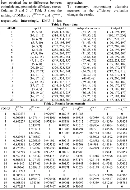
For illustration and clarification the approach, a numerical example is provided. Suppose there are 20 DMUs that each DMU consists of two inputs, one

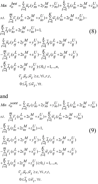
adaptable measure and one output. Data can be seen in Table 1. Data has been given as triangular fuzzy numbers. At first, models (8) and (9) are calculated. The results have been shown in Table 2. The results obtained from model (8) are provided in columns 4-6. As can be found, 6 DMUs, DMU4, DMU5, DMU6, DMU7, DMU16 and DMU17 are optimistic efficient. Also, columns 7-9 show the results obtained from model (9). Column 7 indicates 4 DMUs, DMU1, DMU 11, DMU16 and DMU 20 are pessimistic inefficient. Then, the geometric average efficiencies are computed that are obtained via integrating two different efficiencies. Column 4 of Table 3 indicates them. Afterwards, the arithmetic averages of values of dand 1d, which are obtained from both viewpoints, are calculated and shown in columns 6 and 7 of Table 3, respectively. To compare the results, we consider the adaptable measure as an output factor and calculate the optimistic and pessimistic efficiency scores using the fuzzy expected value approach (Wang and Chin's models [33]. Results are shown in columns 2 and 3 of Table 2. Column 2 indicates the optimistic efficiency results when the adaptable measure is considered as an output. The pessimistic efficiency scores when the adaptable measure is deemed as an output are given in column 3. As can be seen, eWC best_j . ebest_j and eWC worst_j . eworst_j . To illustrate, ebest_j and eworst_j obtain the results

closer than to 1 in contrast to eWC best_j . and

.

WC worst j

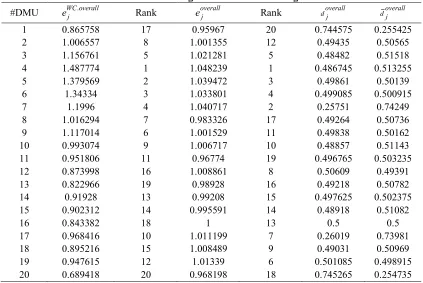
e . Column 2 of Table 3 describes the average efficiency, calculated by the geometric average, when the adaptable measure is considered as an output. The average efficiencies comparisons of two approaches do not display an especial

(8)

pattern. Actually, the varied results have been obtained due to differences between optimistic and pessimistic efficiency scores. Columns 3 and 5 of Table 3 show the ranking of DMUs by eWC average_j . and eaverage_j , respectively. Interestingly, DMU 4 has

obtained the best ranking in both approaches.

To summary, incorporating adaptable measures in the efficiency evaluation changes the results.

Table 1. Fuzzy data

#DMU Input 1 Input 2 Adaptable measure Output 1

1 (5, 5, 5) (470, 475, 480) (34, 35, 36) (194, 195, 196)

2 (10, 11, 13) (314, 315, 318) (48, 50, 52) (196,197, 200)

3 (4, 6, 9) (332, 334, 335) (54, 54, 56) (221, 223, 223)

4 (5, 7, 10) (195, 195, 195) (41, 43, 43) (190, 190, 190)

5 (4, 5, 9) (257, 258, 259) (58, 59, 59) (207, 208, 209)

6 (2, 4, 5) (258, 261, 262) (55, 55, 55) (192, 196, 196)

7 (7, 9, 10) (266, 267, 270) (31, 32, 33) (204, 205, 206)

8 (9, 13, 15) (349, 350, 351) (62, 64, 64) (198, 199, 200)

9 (9, 11, 12) (349, 352, 355) (67, 68, 70) (222, 223, 225)

10 (5, 6, 8) (321, 323, 323) (32, 33, 34) (185, 185, 187)

11 (20, 20, 20) (326, 328, 328) (62, 64, 64) (169, 170, 173)

12 (15, 17, 21) (339, 340, 341) (24, 24, 25) (217, 218, 218)

13 (15, 17, 19) (306, 308, 310) (28, 30, 30) (168, 170, 171)

14 (16, 17, 18) (331, 333, 334) (46,47,48) (198, 200, 201)

15 (9, 12, 16) (315, 316, 318) (39, 41, 41) (186, 187, 189)

16 (17, 17, 17) (244, 245, 247) (14, 14, 14) (170, 170, 170)

17 (3, 4, 5) (310, 310, 310) (19, 20, 21) (183, 185, 185)

18 (16, 19, 24) (236, 237, 238) (36, 38, 38) (170, 170, 170)

19 (16, 17, 18) (279, 281, 283) (25, 25, 27) (182, 183, 184)

20 (18, 21, 24) (363, 363, 364) (22, 23, 25) (167, 168, 170)

Table 2. Results for an example

#DMU eWC best_j . eWC worst_j . ebest_j dbest_j 1dbest_j eworst_j dworst_j 1dworst_j

1 0.749537 1 0.920967 0.48915 0.51085 1 1 0

2 0.709686 1.427614 0.954065 0.50165 0.49835 1.050989 0.48705 0.51295

3 0.842279 1.588662 0.974514 0.48388 0.51612 1.070293 0.48576 0.51424

4 1 2.213471 1 0.48385 0.51615 1.098806 0.48964 0.51036

5 1 1.903211 1 0.51206 0.48794 1.080501 0.48516 0.51484

6 1 1.804562 1 0.51204 0.48796 1.068744 0.48613 0.51387

7 0.823915 1.746587 1 0 1 1.083092 0.51502 0.48498

8 0.796623 1.296539 0.941921 0.50213 0.49787 1.026552 0.48315 0.51685

9 0.851391 1.465507 0.955313 0.51492 0.48508 1.04998 0.48184 0.51816

10 0.720766 1.36826 0.965283 0.48147 0.51853 1.049929 0.49567 0.50433

11 0.851219 1.06428 0.936521 0.50212 0.49788 1 0.49141 0.50859

12 0.657184 1.162342 0.984127 0.4872 0.5128 1.034216 0.52498 0.47502

13 0.565594 1.197453 0.953741 0.48826 0.51174 1.026144 0.4961 0.5039

14 0.64147 1.317405 0.945419 0.50157 0.49843 1.041044 0.49368 0.50632

15 0.60767 1.339817 0.950203 0.48371 0.51629 1.043148 0.49465 0.50535

16 0.711293 1 1 0 1 1 1 0

17 0.886777 1.057571 1 0 1 1.022523 0.52038 0.47962

18 0.736174 1.088617 0.970496 0.48545 0.51455 1.047969 0.49517 0.50483

19 0.668304 1.34366 0.979607 0.49001 0.50999 1.048339 0.51216 0.48784

Table 3. Averages of results and ranking

#DMU eWC overall_j . Rank eoverall_j Rank doverall_j doverall_j

1 0.865758 17 0.95967 20 0.744575 0.255425

2 1.006557 8 1.001355 12 0.49435 0.50565

3 1.156761 5 1.021281 5 0.48482 0.51518

4 1.487774 1 1.048239 1 0.486745 0.513255

5 1.379569 2 1.039472 3 0.49861 0.50139

6 1.34334 3 1.033801 4 0.499085 0.500915

7 1.1996 4 1.040717 2 0.25751 0.74249

8 1.016294 7 0.983326 17 0.49264 0.50736

9 1.117014 6 1.001529 11 0.49838 0.50162

10 0.993074 9 1.006717 10 0.48857 0.51143

11 0.951806 11 0.96774 19 0.496765 0.503235

12 0.873998 16 1.008861 8 0.50609 0.49391

13 0.822966 19 0.98928 16 0.49218 0.50782

14 0.91928 13 0.99208 15 0.497625 0.502375

15 0.902312 14 0.995591 14 0.48918 0.51082

16 0.843382 18 1 13 0.5 0.5

17 0.968416 10 1.011199 7 0.26019 0.73981

18 0.895216 15 1.008489 9 0.49031 0.50969

19 0.947615 12 1.01339 6 0.501085 0.498915

20 0.689418 20 0.968198 18 0.745265 0.254735

5. Conclusions

In real world applications, there are situations that the status of imprecise measures is uncertain from input and/or output viewpoints. Also, conventional DEA models usually evaluate the efficiency from an optimistic point of view. In the current paper, the efficiency scores of DMUs from two aspects, optimistic and pessimistic, have been evaluated where these adaptable variables exist in a fuzzy environment. Then, the overall efficiency of DMUs has been calculated by using the geometric average of efficiencies. Actually, the fuzzy expected value has been used to handle fuzzy DEA models introduced herein in order to handle situations that imprecise and adaptable measures exist.

A numerical example has been used to illustrate the approach. Analysis of the results has shown that the average efficiency scores obtained have changed by incorporating fuzzy adaptable measures.

Also, the overall efficiency calculation and the consideration of both points of view, optimistic and pessimistic, result in more rational and realistic consequences.

Models developed in the current study have been based on constant return to scale technology. However, the approach can be extended for variable returns to scale technology. Moreover, further research might be concentrated on the investigation of the supplier selection problem where adaptable and imprecise variables present. Also, it seems more research is required in determining the overall efficiency in the existence of fuzzy adaptable measures and undesirable factors.

Acknowledgement

References

[1] A. Charnes, W.W. Cooper and E. Rhodes, Measuring the efficiency of decision-making units, European Journal of Operational Research, 2 (1978), 429-444.

[2] Y. M. Wang, K. S. Chin and J. B. Yang, Measuring the performances of decision making units using geometric average efficiency, Journal of the Operational Research Society, 58 (2007), 929-937.

[3] J. K. Sengupta, A fuzzy systems approach in data envelopment analysis,

Computers and Mathematics with

Applications, 24 (1992), 259-266.

[4] A. Hatami-marbini, A. Emrouznejad and M. Tavana, A taxonomy and review of the fuzzy DEA literature: Two decades in the making, European Journal of Operational Research, 214 (2011), 457-472.

[5] A. Emrouznejad and M. Tavana, Performance Measurement with Fuzzy Data

Envelopment Analysis, Berlin and

Heidelberg: Springer, (2014).

[6] C. Kahraman and E. Tolga, Data envelopment analysis using fuzzy concept,

in28th International Symposium on

Multiple-Valued Logic, 38 (1998), 338-343.

[7] P. Guo, H. Tanaka and M. Inuiguchi, Self-organizing fuzzy aggregation models to rank the objects with multiple attributes, IEEE Transctions on Systems, Man and Cybernetics Part A-System and Humans, 30 (2000), 573-580.

[8] S. Lertworasirikul, S.C. Fang, H. L. W. Nuttle and J.A. Joines, Fuzzy data envelopment analysis, in Proceedings of the 9th Bellman Continuum, Beijing,, (2002), 342.

[9] O. Girod, Measuring technical

efficiency in a fuzzy environment, Ph.D. Thesis, Department of Industrial and

Systems Engineering, Virginia Polytechnic Institute and State University,1996.

[10] C. Kao and S. T. Liu, Fuzzy efficiency measures in data envelopment analysis, Fuzzy sets and systems, 113 (2000), 427-437.

[11] Y.M. Wang, R. Greatbanks and J.B. Yang, Interval efficiency assessment using data envelopment analysis, Fuzzy Sets and Systems, 153 (2005), 347-370.

[12] Y. M. Wang, Y. Luo and L. Liang, Fuzzy data envelopment analysis based upon fuzzy arithmetic with an application to performance assessment of manufacturing

enterprises, Expert Systems with

Applications, 36 (2009), 5205-5211.

[13] P. Guo and H. Tanaka, Fuzzy DEA: a perceptual evaluation method, Fuzzy Sets and Systems, 119 (2001), 149{160.

[14] R. Qin, Y. Liu, Z. Liu and G. Wang, Modeling fuzzy DEA with Type-2 fuzzy variable coefficients, Lecture Notes in Computer Science. Springer, Heidelberg, (2009), 25-34.

[15] R. Qin and Y.K. Liu, A new data envelopment analysis model with fuzzy random inputs and outputs, Journal of applied mathematics and computation, 33 (2010), 327-356.

[16] W. D. Cook and J. Zhu, Classifying inputs and outputs in data envelopment analysis, European Journal of operational Research, 180 (2007), 692-699.

[17] M. Toloo, On classifying inputs and outputs in DEA: a revised model, European Journal of Operational Research, 198 (2009), 358-360.

[19] M. Toloo, Alternative solutions for classifying inputs and outputs in data envelopment analysis, Computers and Mathematics with Applications, 63 (2012), 1104-1110.

[20] A. Amirteimoori and A. Emrouznejad, Notes on Classifying inputs and outputs in

data envelopment analysis, Applied

Mathematics Letters, 25 (2012), 1625-1628.

[21] S. Kordrostami and M. Jahani Sayyad Noveiri, Evaluating the Efficiency of Decision Making Units in the Presence of Flexible and Negative Data, Indian Journal of Science and Technology, 5 (2012), 3776-3782.

[22] A. Amirteimoori, A. Emrouznejad and

L. Khoshandam, Classifying exible

measures in data envelopment analysis: A slack-based measure, Measurement, 46 (2013), 4100-4107.

[23] A. Amirteimoori, L. Khoshandam and S. Kordrostami, Recyclable outputs in production process: a data envelopment analysis approach, International Journal of Operational Research, 18 (2013), 62-70.

[24] M. Toloo, Notes on classifying inputs and outputs in data envelopment analysis: A comment, European Journal of operational Research, 235 (2014), 810-812.

[25] S. Kordrostami, G. Farajpour and M. Jahani Sayyad Noveiri, Evaluating the efficiency and classifying the fuzzy data: A DEA based approach, International Journal of Industrial Mathematics, 6 (2014), 321-327.

[26] S. Kordrostami and M. Jahani Sayyad Noveiri, Evaluating the performance and classifying the interval data in data envelopment analysis, International Journal of Management Science and Engineering Management, 9 (2014), 243-248.

[27] W. D. Cook, R. H. Green and J. Zhu, Dual-role factors in data envelopment

analysis, IIE Transactions, 38 (2006), 105-115.

[28] W. C. Chen, Revisiting dual-role factors in data envelopment analysis:

derivation and implications, IIE

Transactions, 46 (2014), 653-663.

[29] L. A. Zadeh, Fuzzy sets, Information and Control, 8 (1965), 338-353.

[30] B. Liu, and Y.K. Liu, Expected value of fuzzy variable and fuzzy expected value

models, IEEE. Transactions. Fuzzy

Systems, 10 (2002), 445-450.

[31] Y. K. Liu and B. Liu, Expected value operator of random fuzzy variable and random fuzzy expected value models, International Journal of uncertainty, fuzziness and knowledge-based systems, 11 (2003), 195-215.

[32] A. Charnes and W.W. Cooper,

Programming with linear fractional

functions, Naval Research. Logistics Quarterly, 9 (1962), 181-186.