A Defined Benefit Pension Fund ALM Model through Multistage Stochastic Programming

International Journal of Finance and Managerial Accounting, Vol.2, No.7, Autumn 2017

1

A Defined Benefit Pension Fund ALM Model

through Multistage Stochastic Programming

Davide Lauria [email protected]

Department of Management, Economics and Quantitative Methods University of Bergamo, Italy

Giorgio Consigli

Department of Management, Economics and Quantitative Methods University of Bergamo, Italy (Corresponding author)

[email protected]

ABSTRACT

We consider an asset-liability management (ALM) problem for a defined benefit pension fund (PF). The PF manager is assumed to follow a maximal fund valuation problem facing an extended set of risk factors: due to the longevity of the PF members, the inflation affecting salaries in real terms and future incomes, interest rates and market factors affecting jointly the PF liability and asset portfolio. The problem is formulated as a stochastic programming problem in discrete time and with a discrete set of relevant future economic and demographic scenarios. In real world applications, this class of decision problems under uncertainty leads to very large scale and complex management problems, due to pending regulatory constraints and the need to preserve the PF funding conditions. Dynamic stochastic programming is shown under such conditions to provide a natural and effective mathematical and numerical approach.

Keywords:

1. Introduction

Asset Liability Management (ALM) is the process of finding optimal policies for long term investors which need to meet future obligations. The implemented strategy should be optimal both with respect to the financial resources and with respect to the liability of the real-life problem subject to a set of management and institutional constraints. In case of Pension funds ALM, the problem is highly stochastic due to the risky nature of future demographic, actuarial and economic variables such as financial returns, liability and macroeconomic indicators. It is so necessary to find a proper set of mathematical tools able to optimise the strategy considering the stochastic implications. Multistage stochastic programming (MSP) is an extension of mathematical programming in which some or all parameters have a stochastic nature. Traditional solutions methods for MSP required a discrete approximation of the underlying probability distribution governing the evolution of the random parameters in order to transform the problem into a deterministic equivalent representation. The deterministic representation can then be solved using traditional optimization algorithms or more specialised solvers which take advantage of the special structure of the problem. Advancements in computer technology and in algorithms efficiency enable increasing opportunities in modelling and solving these problems with long time horizons, a large number of decision variables and constraints and with sophisticated objective functions. As a result, MSP has emerged as a fruitful technique to deal with ALM problems for its flexibility in modelling real life specific features such as, friction markets with transaction costs and taxes, complex regulatory and management constraints and multi-target objective functions.

Areas of applications where MSP has been successfully applied are asset allocation [46, 48], bank management [4, 34], fixed income portfolio management [2, 3, 16], insurance and pension fund companies [6, 7, 8, 11, 14, 17, 25] and minimum guarantee financial products [13]. Typically, dynamic ALM problems are formulated to find the optimal dynamic investment strategy which fulfils a set of constraints and maximise an expected utility function over an investment horizon with a given set of portfolio rebalancing periods. In some models also policy parameters, such as the optimal contribution rate in a pension fund, are considered as variables.

MSP models the presence of arbitrages will lead to unbounded solutions. When instead the short selling in each asset is limited, optimal solutions are obtained but they are biased. Klaassen [31, 32] was the first to show how arbitrage opportunities can bias the optimal solution of a bond selection investment problem with liability. The arbitrage opportunities issue related to the generation of a scenario tree for asset returns has been then considered by other authors. Geyer, Hanke, and Weissensteiner [19, 20] investigate the theoretical relationships between the mean vector and the covariance matrix specifications of the statistical model for asset returns and the existence of arbitrage opportunities. Consiglio, Carollo and Zenios [9] and Staino and Russo [43] proposed two similar moment matching tree generation approaches which directly consider the problem of avoiding arbitrage opportunities.

This paper presents an example of MSP model formulation for an optimal ALM problem for a Defined Benefit (DB) pension plan. Pension plans with defined benefits are determined by formulas taking into account number of years of contributions and the level of earnings for some part of the working career. The amount of contributions deposited by the employee during its active life is generally used only as a condition for benefits. In a typical DB plan a minimum number of contribution years is required to get the life annuity, which is usually a percentage of the last pre-retirement nominal earnings. Sometime the fixed guaranteed monthly benefits are indexed to inflation. The pension fund pays the annuities already matured with the contributions of the actives members, plus the eventually investment returns. The total amount of contributions, plus the investment returns, must be adequate to cover benefit costs. If contributions from employees and employers, plus the investment returns are not adequate to cover the additional benefits earned each year, the unfunded benefit obligation increases, and the funded status of the plan deteriorates. The MSP model provides the optimal investment policy in order to maximise the final portfolio value and at the same time minimise the risk of losses with respect a final portfolio target.

2. Multistage Stochastic Programming

Model

In MSP we define the future uncertainty as an 𝑅𝑑 -valued stochastic process 𝜉 = {𝜉𝑡}𝑡=0𝑇 defined on a

probability space {Ω, ℱ, ℱ𝑡}𝑡=0𝑇 . The atoms of Ω are

sequences of real-valued vectors at discrete time periods 𝑡 ∈ 𝕋, with 𝕋 = {0, 1, … , 𝑇 }. We define

{𝒩𝑡}𝑡=0𝑇 as a sequence of partitions of Ω such that 𝒩0= Ω, 𝒩𝑇= {{𝜔1}, . . . , {𝜔𝑇}}and where each element 𝑛 ∈ 𝒩𝑇 is equal to the union of some

elements in 𝒩𝑡+1 for every 𝑡 < 𝑇. This succession of

partitions of Ω defines uniquely the information structure of the probability space and each σ-algebras

ℱ𝑡 is generated by the partition 𝒩𝑇 and the usual

properties on the filtration hold ℱ = {𝜑, Ω}, ℱ𝑡 ⊂ ℱ𝑡, ∀𝑡 ∈ 𝑇. At the first time 𝑡 = 0 every state 𝜔 ∈ Ω is possible whereas at the final time period 𝑡 = 𝑇 we know exactly which 𝜔 ∈ Ω is the real state of the world. At each intermediate stage 0 < 𝑡 < 𝑇 the investors know that for some subset 𝐴𝑡 of 𝒩𝑡 the true state is some Ω ∈ 𝐴𝑡, but they are not sure which one it is. The probability space can be viewed as a non-recombinant scenario tree and the elements 𝑛of each partition 𝒩𝑡 are called nodes. Every node 𝑛 ∈ 𝒩𝑡 for 𝑡 = 0, . . . , 𝑇 has a unique parent denoted 𝑎 (𝑛) ∈

𝒩𝑡+1 and every node 𝑛 ∈ 𝒩𝑡for 𝑡 = 0, . . . , 𝑇 − 1 has

a non-empty set of child nodes 𝒞(𝑛) ⊂ 𝒩𝑡+1. The probability distribution ℙ is such that ∑𝑛 ∈𝒩𝑇𝑝𝑡= 1

for the terminal stage and 𝑝𝑛= ∑𝑛 ∈ 𝒞(𝑛)𝑝𝑚∀𝑛 ∈ 𝑁𝑡, 𝑡 = 𝑇 − 1, . . . , 0. The conditional probability that the node 𝑚 occurs, given that the parent value is 𝑛 =

𝑎 (𝑚) has occurred, is defined by 𝑝𝑚|𝑛=𝑝_𝑝𝑚 𝑛, with

𝑚 ∈ 𝒞(𝑛). We call the sub-tree associated to the node 𝑛at the stage 𝑡 the one-period tree composed by the node 𝑛and by its child nodes 𝒞(𝑛).

In what follows the asset universe for the pension fund problem is assumed to include a cash account and a set of 𝐼 liquid securities (fixed income securities, equity investments including emerging markets and money market) that can be traded at each decision date

𝑡 = 0, . . . , 𝑇. We denote by 𝑟0= {𝑟0,𝑡}𝑡=0𝑇 the

fund has to pay a net amount of cash determined as the difference between pensions (outflows) and contributions (inflows) and which is assumed driven by two uncertain factors: the inflation and the mortality risks. We represent this uncertain stream of payments by the stochastic process 𝑙 = { 𝑙 𝑡}𝑡=0𝑇 (𝑙has

positive value but is a net expenditure for the pension fund). The net pension payment process 𝑙is obtained from a population model (representing the pension fund members dynamic) driven by a stochastic mortality rate 𝜇 = {𝜇 𝑡}𝑡=0𝑇 and a from a salarymodel

driven by a stochastic inflation process 𝜋 = {𝜋 𝑡}𝑡=0𝑇

and does not depend on the realization of the multivariate asset process. We define 𝑁𝑓,𝛼,𝑡 and 𝑁𝑚,𝛼,𝑡

as the total female (𝑓) and male (𝑚) members aged 𝛼 respectively at 𝑡. We consider two age sets 𝒜 =

20, . . . , 65 and 𝒫 = 66, . . . , 100 which represent respectively the working ages (active) and the ages after retirement (pension), where we have assumed that the retirement age is 66 for both male and female members. At the starting point 𝑡 = 1 we know exactly 𝑁𝑠,𝛼,𝑡, for 𝑠 = 𝑚, 𝑓 and ∀ 𝛼 ∈ 𝒜 ∪ 𝒫. The future population dynamics is modelled by means of a stochastic mortality rate 𝜇 𝛼,𝑡 which states the

percentage of deaths between time 𝑡 − 1 and 𝑡 in a population with age 𝛼. Under these assumptions we can draw the population evolution for 𝑡 = 1, . . . , 𝑇 −

1 as:

(1)

𝑁𝑠,𝛼+1,𝑡+1 = (1 – 𝜇 𝑠,𝛼,𝑡) · 𝑁𝑠,𝛼,𝑡, 𝛼 ∈ 𝒜 ∪ 𝒫, 𝑠 = {𝑚, 𝑓 }.

Once we have specified the population evolution we have to model the salary 𝑤 dynamics for each member, so that we can then derive the processes describing contribution and pension flows. The salary evolution for each individual depends on the age and on the inflation rate: the age-related increase is deterministic and based on a fixed yearly proportion increment 𝜏, whereas the inflation related increase is derived according to the stochastic inflation process 𝜋. The salary dynamic, for 𝑡 = 1, … , 𝑇 − 1, can be then stated as follows:

(2)

𝜔𝑠,𝛼+1,𝑡+1 = 𝜔 𝑠,𝛼,𝑡· ( 1 + 𝜏),

𝛼 ∈ 20, … , 64, 𝑠 = {𝑚, 𝑓 }.

The individual contribution 𝑐𝑠,𝛼,𝑡 of an individual

of sex 𝑠 ∈ 𝑚, 𝑓, aged 𝛼at time 𝑡, for 𝑡 = 1, . . . , 𝑇, is then obtained as the fraction 𝑟𝑐(contribution rate) of the salary at time 𝑡, for 𝑡 = 1, . . . , 𝑇:

(3)

𝑐𝑠,𝛼+1,𝑡+1 = 𝑟𝑐 · 𝑐 𝑠,𝛼,𝑡,

𝛼 ∈ 20, … , 65, 𝑠 = {𝑚, 𝑓 }

The individual pension 𝑃𝑠,𝛼,𝑡 of an individual of sex 𝑠aged 𝛼at time 𝑡, for 𝑡 = 1, . . . , 𝑇, are instead computed as the fraction 𝑟𝑝(pension rate) of the last salary plus an inflation adjustment:

(4)

Ps,α,t = rp· ω s,α−1,t−1, α ∈ 66,s = {m, f }

(5)

Ps,α,t = rp· P s,α−1,t−1, α ∈ 67, … ,100, s = {m, f }

Finally, we can compute the total amount of net pension payments 𝑙𝑡 at time 𝑡 just by aggregating the total contributions 𝐶𝑡 and total pensions 𝑃𝑡 according to

the number of active and passive members of both sexes at time 𝑡:

(6)

𝐶𝑡= ∑ ∑ [𝑐𝛼∈ 𝑠∈ 𝑠,𝛼,𝑡· 𝑁𝑠,𝛼,𝑡]

(7)

𝑃𝑡= ∑ ∑ [𝑐𝛼∈ 𝑠∈ 𝑠,𝛼,𝑡· 𝑁𝑠,𝛼,𝑡] 𝑡 = 1, . . . , 𝑇

(8)

𝑙𝑡= 𝑃𝑡 − 𝐶𝑡 𝑡 = 1, . . . , 𝑇

These I +2 stochastic processes are the elements of

the coefficient vector process {𝜉𝑡}𝑡=0𝑇−1, i.e., 𝜉𝑡 = [𝑟0,𝑡, 𝑟1,𝑡, 𝑟2,𝑡, . . . , 𝑟𝐼,𝑡, 𝑙𝑡], 𝑡 = 0, . . . , 𝑇. We

suppose that the pension fund starts at 𝑡 = 0 with an initial cash amount 𝑥̅𝑖,0 invested in the 𝑖-th asset, for 𝑖 = 1, . . . , 𝐼, and an initial cash surplus of 𝑥̅0,0. The decision process is then defined by a sequence of trading (rebalancing) decisions represented by buying 𝑥𝑖,𝑡+, selling 𝑥𝑖,𝑡−, 𝑖-th asset at times 𝑡, for 𝑖 = 1, . . . , 𝐼, which in turn

will determine the amounts 𝑥𝑖,0, of 𝑖 = 0, . . . , 𝐼, held in each asset after the decisions at time t has been made:

(9)

And

(10)

𝑥𝑖,𝑡(𝜉𝑡) = [1 + 𝑟𝑖,𝑡] · 𝑥𝑖,𝑡−1(𝜉𝑡−1) + 𝑥𝑖,𝑡+(𝜉𝑡) − 𝑥𝑖,𝑡−(𝜉𝑡). 𝑡 = 1, . . . , 𝑇

The rebalancing decisions and the net pension payments affect the amount of cash in the bank account, where we have assumed to have just received the contributions and payed the pensions at the starting time

𝑡. We also suppose fixed transaction costs for 𝜂+ and

𝜂−_{buying and selling one unit of the 𝑖-th asset}

respectively. The cash balance evolution is described as follows. At 𝑡 = 1:

(11) At 𝑡 = 1:

𝑥0,0(𝜉1) = 𝑥̅0,0+ ∑𝐼𝑖=1(1 − 𝜂−) · 𝑥𝑖,0−(𝜉1)− ∑ (1 + 𝜂+_{) · 𝑥}

𝑖,0+(𝜉1), 𝐼

𝑖=1 𝑡 = 0

(12) And for 𝑡 > 0:

𝑥0,𝑡(𝜉𝑡) = [1 + 𝑟0,𝑡] · 𝑥0,𝑡−1(𝜉𝑡−1) + ∑ (1 − 𝜂𝐼𝑖=1 −) · 𝑥𝑖,𝑡−(𝜉𝑡) − ∑ (1 + 𝜂𝐼𝑖=1 +) · 𝑥𝑖,𝑡+(𝜉𝑡), 𝑡 = 1, . . . , 𝑇

The portfolio value 𝑋𝑡 after rebalancing at time 𝑡 is then 𝑋𝑡= ∑𝐼𝑖=0𝑥𝑖,𝑡. We introduce the following risk

measure on the final portfolio value 𝑋𝑇:

(13)

𝜌 (𝑋𝑇) =

𝛽𝐸𝑝 [−𝑋𝑇 ] + (1 − 𝛽) 𝐸𝑃 [𝑚𝑎𝑥 (0, 𝐺𝑇− 𝑋𝑇 ) |𝐹𝑡]

which is defined as a convex combination between the negative of the final port- folio value at T and the negative deviation of the final portfolio value with respect a pre-specified target 𝐺𝑇. The parameter 𝛽

controls the optimiser risk attitude: when 𝛽is set equal to zero negative portfolio value positions are ruled out and we fall in the super hedging case. As we increase the risk parameter toward the unity value more risk the optimiser is willing to take in exchange of a higher expected final return. The DB pension fund manager seeks an optimal investment policy among a defined set of asset classes such that the risk measure 𝜌(𝑋𝑇 ) is minimised.

In a discrete model with a finite number of stages and a discrete partition, where the uncertain parameters are described by a non-recombinant scenario tree, the MSP problem is usually solved by means of its equivalent deterministic representation

form. We define as 𝒩 the set of all nodes at every stage 𝑡, ∀ 𝑡 ∈ 𝕋, and with 𝑥𝑛= [𝑥0,𝑛, 𝑥1,𝑛, … , 𝑥𝐼,𝑛], 𝑥𝑛+= [𝑥1,𝑛+ , … , 𝑥1,𝑛+ ], 𝑥𝑛−= [𝑥1,𝑛− , … , 𝑥1,𝑛− ], the vectors

containing the decisions for all the assets at a given node 𝑛. The liability pricing problem can be formulated as follow:

(14)

ALM Problem

𝑚𝑖𝑛𝑥𝑛,𝑥𝑛+,𝑥𝑛−; ∀ 𝑛 ∈ 𝒩 ∑ 𝑝𝑛(−𝛽𝑋𝑛)

𝑛 ∈ 𝒩𝑇

+ (1 − 𝛽)[𝐺𝑇− 𝑋𝑛]+

𝑠. 𝑡.:

(15)

𝑥𝑖,0= 𝑥̅𝑖,0+ 𝑥𝑖,0+ − 𝑥𝑖,0− 𝑖 = 1, … , 𝐼,

(16)

𝑥0,0= 𝑥̅0,0+ ∑𝐼𝑖=1(1 − 𝜂−) · 𝑥𝑖,0− − ∑𝐼𝑖=1(1 + 𝜂+) · 𝑥𝑖,0+,

(17)

𝑥𝑖,𝑛= [1 + 𝑟𝑖,𝑛] · 𝑥𝑖,𝑎(𝑛)+ 𝑥𝑖,𝑛+ − 𝑥𝑖,𝑛− 𝑖 = 1, … , 𝐼, 𝑛 ∈ 𝒩𝑇, 𝑡 ≥ 1

(18)

𝑥0,𝑛= [1 + 𝑟0,𝑡] · 𝑥0,𝑎(𝑛)+ ∑ (1 − 𝜂𝐼𝑖=1 −) · 𝑥𝑖,𝑛− − ∑ (1 + 𝜂+_{) · 𝑥}

𝑖,𝑛+ − 𝑙𝑛, 𝐼

𝑖=1 𝑛 ∈ 𝒩𝑇, 𝑡 ≥ 1

(19)

𝑋𝑛= ∑𝐼𝑖=0𝑥𝑖,𝑛𝑛 ∈ 𝒩𝑇, 𝑡 ≥ 1

(20)

𝑥𝑖,𝑛+ ≥ 0, 𝑥𝑖,𝑛− ≥ 0𝑖 = 1, … , 𝐼, 𝑛 ∈ 𝒩𝑇, 𝑡 ≥ 1

(21)

𝑥𝑖,𝑛≥ 0𝑖 = 1, … , 𝐼, 𝑛 ∈ 𝒩𝑇, 𝑡 ≥ 1

A deterministic equivalent representation is possible because we have completely described the future uncertainty with a finite set of possible realisations by means of the scenario tree process

{𝜉𝑡}𝑡=0𝑇 with 𝜉𝑡= [𝑟𝑡, 𝑙𝑡]. A crucial issue for a successful implementation of multistage stochastic programming models is the specification of the mass points 𝑟𝑛 and 𝑙𝑛 for 𝑛 ∈ 𝒩𝑡 and 𝑡 = 0, … , 𝑇.

fund scheme. The econometric model can be defined both in discrete and in continuous time. The second step is to find an efficient technique to specify the scenario tree {𝜉𝑡}𝑡=0𝑇 which represent the possible evolution of the estimated econometric model, and which will be used as an input in the equivalent deterministic representation problem. The greater the number of nodes in the scenario tree, the more accurate is the approximation. However, increasing the number of nodes also increases the computational effort to solve the problem. This consideration implies that we face a trade-off between the accuracy of the risk representation and the practical problem solvability. An important question is the extent to which the approximation error in the event tree will bias the optimal solutions of the model. Different approaches to generate scenario trees for have been proposed, see [12] and the references therein for a quite recent critical overview.

3. Case Study

In this section we perform the optimal portfolio allocation on a simple case study based on a DB pension fund problem. We consider an investment period of seven years 𝑇 = 7 on an asset universe composed by seven risky and liquid securities plus a cash account. The seven securities considered are: Barclays Euro Government All Mats. Index, FTSE Global Government US All Mats. Index, FTSE Euro Emerging Markets All Mats. Index, S&P 500 Composite Price Index, Morgan Stanley Capital international EMU and the MSCI Emerging Markets Price Index. The portfolio rebalancing periods are defined by the time index set 𝑇 = {0, 1, 3, 5, 7}. The first task is to determine the values for the tree processes 𝑟𝑡and 𝑙𝑡 for 𝑖 = 0, . . . , 𝐼, which will form the input parameters for the ALM Problem. The topology of such a tree will be uniquely determined by the set

𝑁 = {1, ℕ1, ℕ2, ℕ3, ℕ4} describing the number of nodes in each sub-tree at a given decision stage. Here we consider the case 𝑁 = {1, 10, 10, 10, 10}.

In order to obtain the evolution of the short interest rate and the inflation rate a parsimonious vector autoregressive (VAR) model of order one was developed with four state variables in nominal values: the euro area output-gap, the euro area one-year consumer price index variations, the 12 months Euribor rate and the ten years euro government

benchmark return. The former represents the risk free stochastic interest rate which will be used to model the cash account return and to discount the cash flows whereas the letter will be used return and to discount the cash flows whereas the letter will be used to model the salary and the pension dynamics. We use quarterly data over the period from 1998 to 2008 to calibrate the parameters and from the last quarter of 2008 to the first quarter of 2015 for the out-of-sample analysis. The pension fund population evolution is constructed on the basis of a stochastic mortality model [35] and it is used, along with the inflation rate, to define the actuarial pension fund variables and their dynamics. An extensively description of the model can be found in [29]. Historical asset returns from 31-January-2009 to 31-December-2015 are obtained from the Thompson Data Stream database with monthly frequency and all quoted in euro currency. Each of the seven securities dynamic is modelled independently fitting a Glosten, Jagannathan, and Runkle (GJR) model [21] and the correlation among them is reconstructed by modelling innovations with a t-copula.

The macroeconomics, actuarial and asset models are used to simulate a large scenario fan 𝜉 ̅𝑠=

[𝜉̅0𝑠, … , 𝜉̅𝑇𝑠 ], 𝑠 = 1, . . . , 𝑆 with independent trajectories. The scenario tree {𝜉𝑡}𝑡=0𝑇 will be constructed in a forward fashion using as inputs the scenario fan trajectories, 𝑠 = 1, . . . , 𝑆, and the given symmetric branching structure ℕ describing the number of nodes in each sub-tree at each stage 𝑡. The branching structure is defined by the user, but it must be such that 𝑁𝑡≥ 𝐼 + 1 to satisfy the necessary condition for the absence of arbitrages. The method relies on the application of the Sequential Wasserstein Distance Minimisation (SMWD) algorithm [12], along with a moment matching problem, which also considers a set of constraints to directly avoid arbitrage opportunities [9, 43], to generate each sub-tree starting from the root node. Since the moment matching problem is highly non-linear a set of transformations and an approximation procedure have been used in order to solve it more efficiently (see [29] for a detailed description).

and the expected sum of future net payments Γ0 under the real-world probability measure ℙ:

Γ0= 𝑋 ̅0− ∑𝑇𝑡=0𝔼[𝑙𝑡].

We suppose the pension fund manager seeks a minimal investment return of 3% per annum along all the horizon 𝑇:

𝐺𝑡= Γ0(1 + 0.003)𝑇

The optimal solution of the ALM Problem is computed for different values of the risk parameter β from 0 to 0.5 with a step of 0.05. The models have been implemented on a 2,8 GHz Intel Core i7 machine, with a RAM of 16 GB 1600 MHz DDR3, running OS X Yosemite as operating system. The data pre-processing, the econometric model and the input specification for the optimization problems have been developed using the commercial soft- ware package MATLAB R2014b (The MathWorks, Inc., Natick, Massachusetts, United States). All the optimization problems are instead solved using the interior-point solver developed in the software MOSEK 7 which has

been directly linked to the MATLAB software through a MEX file. The computational time to generate a tree with branching structure [1 10 10 10 10], (1e4 final nodes) is 506,75 seconds. The ALM Problem optimisation instance is a linear program with 266.663 scalar variables and 111.109 constraints solved in 299,12 seconds.

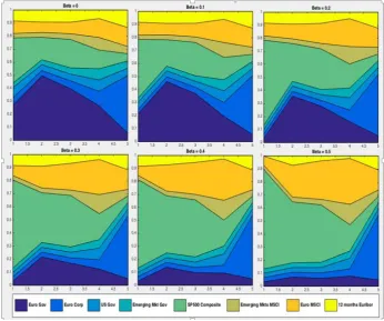
Figure (1) shows the portfolio composition as time goes by for different value of the risk parameter β. It is clear that as we increase the risk attitude the optimizer gradually shifts the asset allocation toward riskier securities.

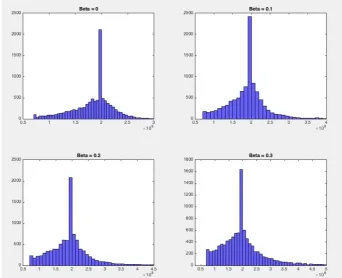
This effect can be also understood by looking at the final portfolio value 𝑋T distribution, which is stored in Figure (3): as β increases distribution left tail becomes fatter. The increasing risk tolerance produces a higher expected portfolio value and at the same time a higher expected semi-deviation with respect the target 𝐺T. This can be appreciated by looking at Figure (2) where expected negative deviations from the target (x-axis) and expected final portfolio value (y-axis) for all different values of β are plotted.

Figure 2: Efficient Frontier

4. Conclusion

In this work a simple application of MSP to an ALM problem faced by a DB pension Fund has been presented. From the problem formulation to the definition of an optimal dynamic strategy based on fixed income and equity allocations in the US and Europe. The key steps from identifying the financial and economic drivers of a pension fund management problem, to the definition of a statistical model of their evolution and their integration in a large-scale structured stochastic linear program, solvable relying on efficient linear algorithms have been considered as constituents of an efficient decision support tool for long-term asset-liability management. The practical adoption of those tools requires both model validation and accurate scenario analysis, including out-of-sample back testing approaches.

References

1) Beraldi P., De Simone F., Violi A. (2010). Generating scenario trees: a parallel integrated simulation optimization approach, Comput. Appl. Math., 233, pp. 2322-233.

2) Beraldi, P., Consigli, G., De Simone, F., Iaquinta, G. and Violi, A. (2011). Hedging market and credit risk in corporate bond portfolios, In Handbook on Stochastic Optimization Methods in Finance and Energy, Fred Hillier International Series in Operations Research and Management Science, edited by M. Bertocchi, G. Consigli and M. Dempster, Chapter 4, pp. 73-98 (Springer: New York).

3) Bertocchi M., Dupaˆcová J., Moriggia V. (2007). Bond portfolio management via stochastic programming, In Handbook of asset and liability management, vol. 1, Theory and methodology, ed. S. A. Zenios and W. T. Ziemba, 305-336. 4) Castro J. (2009). A stochastic programming

approach to cash management in banking, European Journal of Operational Research,192, 963-974. 5) Chiralaksanakul A., Morton D. P. (2004). Assessing

policy quality in multi-stage stochastic

programming, Stochastic Programming E-Print Series 12.

6) Consigli, G., Dempster, M.A.H. (1998).

Dynamic stochastic programming for asset-liability management, Ann. Oper. Res. 81, 131-161.

7) Consigli G., di Tria M., Gaffo M., Iaquinta G., Moriggia V., Uristani A. (2011). Dynamic Portfolio Management for Property and Casualty

Insurance. In Handbook on Stochastic

Optimization Methods in Finance and Energy, Fred

Hillier International Series in Operations Research and Management Science, edited by M. Bertocchi, G. Consigli and M. Dempster, Chapter 5, pp. 99-124, Springer: New York.

8) Consiglio A., Cocco F., Zenios S.A. (2008). Asset and liability modelling for participating policies with guarantees, European Journal of Operational Research 186, 380-404.

9) Consiglio A., Carollo A., Zenios S.A. (2016). A parsimonious model for generating arbitrage-free scenario trees, Quantitative Finance, 01, Vol.16(2), p.201-212.

10)Dempster M. A. H., Germano M., Medova E. A., and Villaverde M. (2003). Global asset liability

management, British Actuarial Journal, 9

(1):137195 Part c.

11)Dempster M.A.H., Germano M., Medova E., Murphy J., Ryan D., Sandrini F. (2009). Risk Profiling Defined Benefit Pension Schemes, The Journal of Portfolio Management, Vol.35(4), pp.76-93.

12)Dempster M. A. H., Medova E. A., Yong Y. S. (2011). Comparison of Sampling Methods for Dynamics Stochastic Programming, Stochastic Optimization Methods in Finance and Energy, Ch. 16, Springer.

13)Dempster M. A. H., Medova E. A., Rietbergen M. I., Sandrini F., Scrowston M. (2011). Designed Minimum Guaranteed Return Funds, Stochastic Optimization Methods in Finance and Energy, Ch. 2, Springer.

14)Dondi G. and Herzog F. (2007). Dynamic Asset and Liabilities Management for Swiss Pension

Funds, Handbook of Asset and Liability

Management Volume 2, Ch.20.

15)Dupaˆcová J., Consigli G., Wallace S. W. (2000). Scenarios for multistage stochastic programs, Annals of Operations Research.

16)Dupaˆcová, J., Bertocchi, M. (2001). From data to model and back to data: A bond portfolio management problem, European Journal of Operational Research 134, 261-278.

17)Dupaˆcová J., Polìvka J. (2009). Asset-liability-management for Czech pension funds using stochastic programming, Annals of Operations Research, Vol.165(1), pp.5-28.

18)Geyer A., Ziemba W. T. (2008). The Innovest Austrian Pension Fund Financial Planning Model InnoALM, Operations Research, Vol.56(4), p.797- 810.

19)Geyer A., Hanke M., Weissensteiner A. (2014). No-arbitrage bounds for financial scenarios, European Journal of Operational Research, 236(2), 657-663. 20)Geyer A., Hanke M., Weissensteiner A. (2014).

No-Arbitrage ROM simulation, Journal of

21)Glosten L., Jagannathan R., Runkle D. (1993). Relationship between the expected value and volatility of the nominal excess returns on stocks, Journal of Finance, 48, 1779-1802.

22)Gülpinar N., Rustem B., Settergren R. (2004). Simulation and optimization approaches to scenario tree generation, Journal of Economic Dynamics and Control, Vol.28(7), pp.1291-1315. 23)Heitsch H., Romisch W. (2005). Generation of

multivariate scenario trees to model stochasticity in power management, IEEE St. Petersburg Power Tech.