S. Descombes, B. Dussoubs, S. Faure, L. Gouarin, V. Louvet, M. Massot, V. Miele, Editors
VLASOV ON GPU (VOG PROJECT)
∗,∗∗,∗∗∗M. Mehrenberger
1, C. Steiner
2, L. Marradi
3, N. Crouseilles
4, E.
Sonnendr¨
ucker
5et B. Afeyan
6R´esum´e. Ce travail concerne la simulation num´erique du mod`ele de Vlasov-Poisson `a l’aide de m´ethodes semi-Lagrangiennes, sur des architectures GPU. Pour cela, quelques modifications de la m´ethode traditionnelle ont dˆu ˆetre effectu´ees. Tout d’abord, une reformulation des m´ethodes semi-Lagrangiennes est propos´ee, qui permet de la r´e´ecrire sous la forme d’un produit d’une matrice circu-lante avec le vecteur des inconnues. Ce calcul peut ˆetre fait efficacement grˆace aux routines de FFT. Actuellement, le GPU n’est plus limit´e `a la simple pr´ecision. N´eanmoins, la simple pr´ecision reste int´eressante pour des raisons de performance et de m´emoire disponible. Afin de contourner le probl`eme de la simple pr´ecision, une m´ethode de typeδf est alors utilis´ee. Ainsi, un code Vlasov-Poisson GPU permet de simuler et de d´ecrire avec un haut degr´e de pr´ecision (grˆace `a l’utilisation de reconstructions d’ordre ´elev´e et d’un grand nombre de points de l’espace des phases) des cas tests acad´emiques mais aussi des ph´enom`enes physiques pertinents, comme la simulation des ondes KEEN.
Abstract. This work concerns the numerical simulation of the Vlasov-Poisson equation using semi-Lagrangian methods on Graphics Processing Units (GPU). To accomplish this goal, modifications to traditional methods had to be implemented. First and foremost, a reformulation of semi-Lagrangian methods is performed, which enables us to rewrite the governing equations as a circulant matrix operating on the vector of unknowns. This product calculation can be performed efficiently using FFT routines. Nowadays GPU is no more limited to single precision; however, single precision may still be preferred with respect to performance and available memory. So, in order to be able to deal with single precision, aδf type method is adopted which only needs refinement in specialized areas of phase space but not throughout. Thus, a GPU Vlasov-Poisson solver can indeed perform high precision simulations (since it uses very high order of reconstruction and a large number of grid points in phase space). We show results for more academic test cases and also for physically relevant phenomena such as the bump on tail instability and the simulation of Kinetic Electrostatic Electron Nonlinear (KEEN) waves.
∗Thanks to Edwin Chacon-Golcher, Philippe Helluy, Guillaume Latu, Pierre Navaro for fruitful discussions and helps
∗∗ Thanks to the CEMRACS organizers and participants for the nice stay
∗∗∗ This work was carried out within the framework the European Fusion Development Agreement and the French Research
Federation for Fusion Studies. It is supported by the European Communities under the contract of Association between Euratom and CEA. The views and opinions expressed herein do not necessarily reflect those of the European Commission.
1 IRMA, Universit´e de Strasbourg, 7, rue Ren´e Descartes, F-67084 Strasbourg & INRIA-Nancy Grand-Est, projet CALVI,
e-mail :[email protected].
2 IRMA, Universit´e de Strasbourg, 7, rue Ren´e Descartes, F-67084 Strasbourg & INRIA-Nancy Grand-Est, projet CALVI,
e-mail :[email protected].
3LIPHY, Universit´e Joseph Fourier, 140, avenue de la Physique, F-38402 Saint Martin d’H`eres, e-mail : [email protected]. 4INRIA-Rennes Bretagne Atlantique, projet IPSO & IRMAR, Universit´e de Rennes 1, 263 avenue du g´en´eral Leclerc, F-35042
Rennes, e-mail :[email protected].
5 Max-Planck Institute for plasma physics, Boltzmannstr. 2, D-85748 Garching, e-mail :[email protected]. 6 Polymath Research Inc., 827 Bonde Court, Pleasanton, CA 94566, e-mail :[email protected].
c
EDP Sciences, SMAI 2013
Introduction
At the one body distribution function level, the kinetic theory of charged particles interacting with electro-static fields and ignoring collisions, may be described by the Vlasov-Poisson system of equations. This model takes into account the phase space evolution of a distribution function f(t, x, v) wheret ≥0 denotes time, x
denotes space andvis the velocity. Considering one-dimensional systems leads to the 1D×1DVlasov-Poisson model where the solutionf(t, x, v) depends on timet≥0, spacex∈[0, L] and velocityv∈R. The distribution
functionf satisfies
∂tf +v∂xf+E∂vf = 0, (1)
whereE(t, x) is an electric field. Poisson’s law dictates that the charged particle distribution must be summed over velocity to render the self-consistent electric field as a solution to the Poisson equation:
∂xE= Z
R
f dv−1. (2)
To ensure the uniqueness of the solution, we impose to the electric field a zero mean conditionRL
0 E(t, x)dx= 0.
The Vlasov-Poisson system (1)-(2) requires an initial conditionf(t = 0, x, v) = f0(x, v). We will restrict our
attention to periodic boundary conditions in space and vanishingf at large velocity.
Due to the nonlinearity of the self-consistent evolution of two interacting fields, in general it is difficult to find an analytical solution to (1)-(2). This necessitates the implementation of numerical methods to solve it. Historically, progress was made using particles methods (see [4]) which consist in advancing in time macro-particles through the equations of motion whereas the electric field is computed on a spatial mesh. Despite the inherent statistical numerical noise and their low convergence, the computational cost of particle methods is very low even in higher dimensions which explains their enduring popularity. On the other hand, Eulerian methods, which have been developed more recently, rely on the direct gridding of phase space (x, v). Eulerian methods include finite differences, finite volumes or finite elements. Obviously, these methods are very demanding in terms of memory, but can converge very fast using high order discrete operators. Among these, semi-Lagrangian methods try to retain the best features of the two approaches: the phase space distribution function is updated by solving backward the equations of motion (i.e. the characteristics), and by using an interpolation step to remap the solution onto the phase space grid. These methods are often implemented in a split-operator framework. Typically, to solve (1)-(2), the strategy is to decompose the multi-dimensional problem into a sequence of 1Dproblems. We refer to [2,6,9,12,14,15,19,24] for previous works on the subject.
The main goal of this work is to use recent GPU devices for semi-Lagrangian simulations of the Vlasov-Poisson system (1)-(2). Indeed, looking for new algorithms that are highly scalable in the field of plasmas simulations (like tokamak plasmas or particle beams), it is important to mimic plasma devices more reliably. Particle methods have already been tested on such architectures, and good scalability has been obtained as in [5,30]. We mention a recent precursor work on the parallelization in GPU in the context of a gyrokinetic eulerian code GENE [13]. Semi-Lagrangian algorithms dedicated to the simplified setting of the one-dimensionnal Vlasov-Poisson system have also recently been implemented in the CUDA framework (see [22,25]). In the latter two works, in which the interpolation step is based on cubic splines, one can see that the speedup can reach a factor of
×80 in certain cases. Here, we use higher complexity algorithms, which are based on the Fast Fourier Transform (FFT). We will see that our GPU simulations will directly benefit from the huge acceleration obtained for the FFT on GPU. They are thus also very fast enabling us to test and compare different interpolation operators (very high order Lagrangian or spline reconstructions) using a large number of grid points per direction in phase space.
big enough. Note also that the proof of convergence of such numerical schemes can be obtained following [3,7]. Due to the fact that such matrices are diagonalizable in a Fourier basis, the matrix vector product can be performed efficiently using FFT. In this work, Lagrange polynomials of various odd degrees (2d+ 1) and B-spline of various degree k have been tested and compared. Another advantage of the matrix-vector product formulation is that the numerical cost is almost insensitive to the order of the method. Finally, since single precision computations are preferable to get maximum performance out of a GPU, other improvements have to be made to the standard semi-Lagrangian method. To achieve the accuracy needed to observe relevant physical phenomena, two modifications are proposed: the first is to use aδf type method following [22]. The second is to impose a zero spatial mean condition on the electric field. Since the response of the plasma is periodic, this is always satisfied.
The rest of the paper is organized as follows. First, the reformulation of the semi-Lagrangian method using FFT is presented for the numerical treatment of the doubly periodic Vlasov-Poisson model. Then, details of the GPU implementation are given, highlighting the particular modifications that were necessary in order to use GPUs with single precision. We then move on to show numerical results. These involve several comparisons between the different methods and orders of numerical approximation and their performances on GPU and CPU on three canonical test problems.
1.
FFT implementation
In this section, we give an explicit formulation of semi-Lagrangian schemes for the solution of the Vlasov-Poisson system of equations in the doubly periodic case using circulant matrices. First, the classical directional Strang splitting (see [9,27]) is recalled. Then, the problem is reduced to a sequence of one-dimensional constant advections; a circulant-matrix formulation is proposed, for which the use of Fast Fourier Transform is very well suited; it can be applied for many methods, with arbitrary order of interpolation.
1.1.
Strang-splitting
For the Vlasov-Poisson set of equations (1)-(2), it is natural to split the transport in thex-direction from the transport in the v-direction. Moreover, this also corresponds to a splitting of the kinetic and electrostatic potential part of the Hamiltonian |v|2/2 +φ(t, x) where the electrostatic potentialφ is related to the electric
field throughE(t, x) =−∂xφ(t, x).
For plasmas simulations, even when high order splittings are possible (see [11] and references therein), the second order Strang splitting is a good compromise between accuracy and simplicity, which explains its popu-larity. Due to filamentation, even if high order scheme and fine grid is used in space, the error is generally more important in space than in time. On the other hand, the use of high order splitting is a possible option, which can be managed easily and will probably have the capability of enhancing the results and/or diminishing the cost of the simulation.
Starting from time tn =n∆t and assuming that fn ' f(tn,·,·) and En 'E(tn,·) are known, the Strang splitting is composed of three steps plus an update of the electric field before the advection in thev-direction
(1) Transport inv over ∆t/2: computefn,?(x, v) =g(∆t/2, x, v) by solving
∂tg(t, x, v) +En(x)∂vg(t, x, v) = 0,
with the initial conditiong(0, x, v) =fn(x, v).
(2) Transport inxover ∆t: computefn,??(x, v) =g(∆t, x, v) by solving
∂tg(t, x, v) +v∂xg(t, x, v) = 0,
with the initial conditiong(0, x, v) =fn,?(x, v). Update of electric fieldEn+1(x) by solving∂
xEn+1(x) = R
(3) Transport inv over ∆t/2: computefn+1(x, v) =g(∆t/2, x, v) by solving
∂tg(t, x, v) +En+1(x)∂vg(t, x, v) = 0,
with the initial conditiong(0, x, v) =fn,??(x, v).
One of the main advantages of this splitting is that the algorithm reduces to solving a series of one-dimensional constant coefficient advections. Indeed, considering the transport along the x-direction, for each fixed v, one faces a constant advection. The same is true for thev-direction since for each fixedx, En does not depend on the advected variablev. We choose to start with the advection in v, which permits to get the electric field at integer multiples of time steps. The third step of thenthiteration could be merged with step (1) of the (n+ 1)th iteration, but we do not resort to this short cut here.
1.2.
Constant advection
In this part, a reformulation of semi-Lagrangian methods is proposed, in the case of constant advection equations with periodic boundary conditions. Let us consider u= u(t, x) to be the solution of the following equation for a given c∈R:
∂tu+c∂xu= 0, u(t= 0, x) =u0(x),
where periodic boundary conditions are assumed inx∈[0, L]. The continuous solution satisfies for allt, s≥0 and allx∈[0, L]: u(t, x) =u(s, x−c(t−s)). Let us mention thatx−c(t−s) has to be understood moduloL
since periodic boundary conditions are being considered.
Let us consider a uniform mesh within the interval [0, L]: xi =i∆x fori = 0, . . . , N and ∆x=L/N. We also introduce the time step ∆t=tn+1−tn forn∈N. Note that we haveun0 =unN. By setting
un =
un 0 .. . .. .
unN−1
, uni ≈u(tn, xi), (3)
the semi-Lagrangian scheme reads uni+1 = πun(x
i−c∆t) where π is a piecewise polynomial function which interpolatesun
i fori = 0, . . . , N −1: π(xi) =uni. This can be reformulated intoun+1 =Aun where A is the matrix defining the interpolation. Periodic boundaries imply that the matrixAis circulant:
A=C(a0, a1, ..., aN−1) :=
a0 a1 . . . aN−1 aN−1 a0 a1 . . . aN−2
. .. . .. . .. . .. . .. . .. . .. . .. . .. . ..
a1 . . . aN−1 a0 (4)
Obviously, this matrix depends on the choice of the polynomial reconstructionπ. In the following, some explicit examples are shown.
Examples of various methods and orders of interpolation
We have to evaluate πun(x
i−c∆t). Letβ :=−c∆t/∆xbe the normalized displacement which can be written in a unique way asβ =b+b? with (b, b?)∈
tn tn+1
xi
xi−c∆t
xi∗ xi∗+1
un
i∗ un+1 uni∗+1
i
uni+1'u(tn+1, xi) =u(tn, xi−c∆t)
(1) Lagrange 1. The nonvanishing terms of the matrixAare:
ab= 1−b?, ab+1=b?.
(2) Lagrange 2d+ 1 (with 2d+ 1≤N−1). The nonvanishing terms of matrix are :
∀j∈ {−d, . . . , d+ 1}, ab+j = d+1 Y
k=−d, k6=j b?−k
j−k.
(3) B-Spline of degreek. We defineBk
i(x) the B-spline of degreekon the mesh (xi)i by the following recurrence:
B0i(x) =1[xi,xi+1[(x), B k i(x) =
x−xi k∆x B
k−1 i (x) +
1−x−xi+1 k∆x
Bik+1−1(x).
Then, in this case, the nonvanishing terms of the matrixAare:
A=M× C(0, . . . ,0
| {z } N−k
, Bk0(x1), Bk0(x2), . . . , B0k(xk)
| {z }
k
)−1,
where the nonvanishing terms of the circulant matrixM are:
∀j∈ {0, . . . , k}, mb−j=Bk0(xj+b?).
Now, starting from this reformulation, the algorithm reduces to a matrix vector product at each time step. Since the matrices are circulant, this product can be performed using FFT. Indeed, circulant matrices are diagonalizable in Fourier space [18] so that
A=U DU?,
where √1
NU is unitary (U
?denotes the adjoint matrix of U) andD is diagonal. They are given by
Um,k = e−2iπmk/N, m, k= 0. . . N−1,
Dm,m = N−1
X
k=0
ake−2iπmk/N, m= 0, ..., N−1.
The product ofU by a vector v∈RN can then be obtained performing the Fast Fourier Transform ofv. In the same way,U?vcan be obtained by computing the inverse Fourier Transform of v.
The product matrix vectorAun=U DU?un is then computed following the algorithm: (1) ComputeU?un by calculating ˜u= FFT−1(un).
(4) ComputeAun by calculating FFT(w).
The complexity of the algorithm is thenO(NlogN), independently of the degree of the polynomial reconstruc-tion.
2.
CUDA GPU implementation
From the Strang-splitting and the constant advection, we can easily define the 2Dalgorithm. The unknowns are
fi,jn 'f(tn, xi, vj), xi=xmin+i∆x, vj=vmin+j∆v, i= 0, . . . , Nx−1, j= 0, . . . , Nv−1,
with ∆x= (xmax−xmin)/Nx, ∆v = (vmax−vmin)/Nv,and Nx, Nv ∈N∗. We use kernels on GPU by using
existing NVIDIA routines for FFT, transposition and scalar product. Note that such a choice has also been made in the more difficult context [13]. We would have liked to use OPENCL (as done in [10]) in order not be attached to NVIDIA cards; but we had difficulties to get the friendly well-documented features of NVIDIA, especially for the FFT.
FFTs are computed using the cufft library. For transposition, different possible algorithms are pro-vided from CUDA samples (see http://docs.nvidia.com/cuda/cuda-samples/index.html#matrix-transpose). For this step, the condition N =Nx =Nv is always required We also have that N is a power of 2, for the FFT step. In order to compute charge density
ρ(t, x) =
Z
f(t, x, v)dv'∆v Nv−1
X
j=0
f(t, x, vj),
we adapt theScalarProdGPUroutine from CUDA samples (seehttp://docs.nvidia.com/cuda/cuda-samples/index. html#scalar-product), since we have
Nv−1 X
j=0
f(t, x, vj) =hu, vi, withu= (f(t, x, v0), . . . , f(t, x, vNv−1)), v= (1, . . . ,1),
andh·,·iis the scalar product.
We also write a kernel on GPU for computing coefficients of the A matrix. An analytical formula is used for each coefficient ai. In the case of Lagrange interpolation of degree 2d+ 1, the complexity switches from O(N d) toO(N d2) operations because of a rewritten CPU divided differences based algorithm which cannot be parallelized.
The main steps of the algorithm are :
• Initialization: the initial condition computed on CPU and transferred to GPU
• Computation of initial charge densityρon GPU by usingScalarProd
• Transfer ofρto CPU
• Computation of the electric fieldE on CPU
• Time loop
1. ∆t/2 advection inv with FFT on GPU
2. Transposition in order to pass into thex-direction on GPU 3. ∆t advection in thexdirection with FFT on GPU
4. Transposition in order to pass into thev-direction on GPU 5. Computation ofρon GPU by usingScalarProd
6. Transfer ofρto CPU
Remarque 2.1. The electric field is computed on CPU, for simplicity; we have not made the effort to translate the code in GPU. We expect not to have a real improvement on the performance by computing the electric field on GPU; the amount to transfer is negligible (the size isO(N)) compared to the advection (the size isO(N2)).
Some details on the implementation
We list here the CUDA kernel calls for information and give some descriptions of the variables.
//for transposition
transposeNoBankConflicts<<<grid, threads>>>(d_odata, f_d, N, N, 1); copy<<<grid, threads>>>(f_d, d_odata, N, N, 1);
//for advection
//for going to complex data
real_to_complex<<<grid, threads>>> (f_d, f_complex_d, N); //for matrix computation: from alpha_d and i0_d returns w_d
compute_coefficients<<<grid, threads>>> (w_d, alpha_d, i0_d, N, degree); cufftExecZ2Z (plan1d, w_d, w_d, CUFFT_FORWARD);
//forward fft
cufftExecZ2Z (plan1d, f_complex_d, f_complex_d, CUFFT_FORWARD); //for multiplication in Fourier space
mult_complex_array<<<grid, threads>>> (f_complex_d, w_d, N); //backward fft
cufftExecZ2Z (plan1d, f_complex_d, f_complex_d, CUFFT_INVERSE); //for going back to real data and multiply by scale factor
complex _to_real_scaled<<<grid, threads>>> (f_complex_d, f_d, N, scale);
//for computation of charge density
compute_sum_v<<<grid_rho, threads_rho>>> (rho_d, f_d, N);
The variablesf d, d odataare real arrays of sizeN2;f d represents the distribution functionf.
The variables w d, f complex d are complex arrays of size N2; w d represents the matrix of coefficients. In Fourier space, we then only need to make the multiplication terms by terms with f complex d, the complex Fourier transform of f.
The variable i0 d (resp. alpha d) is an integer (resp. real) array of sizeN; its elements are b (resp. b∗), for each of the N constant advections.
The variabledegreeis an integer, that representsd, that stands here for the Lagrange interpolation of degree 2d+ 1.
The variablescaleis a real number that is set to 1/N for FFT scaling purpose.
The variable plan1dis a type that initializes the FFT, so that the FFT is applied N times for vectors of size
N, which are stored contiguously in memory. For this, we just have to make the following call once for all:
cufftPlan1d( &plan1d, N, CUFFT_Z2Z, N);
This explains why the transposition of the data are necessary.
The variablerho dis a real array of sizeN, which stores the charge densityρ. The variablesgrid, threadsandgrid rho, threads rhoare initialized as follows:
dim3 grid(N/TILE_DIM, N/TILE_DIM), threads(TILE_DIM,BLOCK_ROWS); dim3 grid_rho(N/TILE_DIM, 1), threads_rho(TILE_DIM,1);
3.
Questions about single precision
In principle, computations on GPU can be performed using either single or double precision. However, the numerical cost becomes quite high when one deals with double precision (we will see in our case, that the cost is generally a factor of two) and is not always easily available across all platforms. Note that in [13] and [25], only double precision was used. Discussions about single precision have already been presented in [22]. Hereafter, we propose two slight modifications of the semi-Lagrangian method which enable the use of single precision computations while at the same time recovering the precision reached by a double precision CPU code.
3.1.
δf
method
Theδfmethod consists on a scale separation between an equilibrum and a perturbation so that we decompose the solution as
f(x, v) =δf(x, v) +feq(v), feq(v) = √1
2πexp(−v 2/2).
Then, we are interested in the time evolution ofδf which satisfies
∂tδf+v∂xδf+E∂v[feq+δf] = 0.
The Strang splitting presented in subsection 1.1 is modified since we advect δf instead of f. Since feq only depends onv, advections inxare not modified. Now we can rewrite thev-advection as
∂t[feq+δf] +En∂v[feq+δf] = 0,
with the initial conditionfeq+δfn,?. This means that (feq+δf) is preserved along the characteristics (feq+
fn,??)(x, v) = (feq+fn,?)(x, v−∆tEn(x)). We then deduce that
δfn,??(x, v) =δfn,?(x, v−∆tEn(x)) +feq(v−∆tEn(x))−feq(v).
which provides the update ofδf for the v-advection. Note that feq(v−∆tEn(x)) is an evaluation and not an
interpolation.
Remarque 3.1. We use here the standard Gaussian feq, because in our test cases, we are not far from this equilibrium. In the bump on tail test case, at initial time, we are nearer of another (unstable) equilibrium: there is another Gaussian, the bump, which is however small and does not remain constant in time; thus we have not found worth enough to adaptfeqto that equilibrium. It may be interesting to look for situations, where we are
not far from another equilibrium (which may even evolve in time) and see how to adapt the procedure. Note that we explicitely use here that feqdoes not depend onx.
3.2.
The zero mean condition
The electric field is computed from (2). Note that the right hand side of (2) has zero mean, and the resulting electric field has also zero mean. This is true at the continuous level; however when we deal with single precision, a systematic cumulative error could occur here. In fact, it is also true in the double precision case, but the influence is quite less significative, as we will see on the numerical results. In order to prevent this cumulative error phenomenon, we can enforce the zero mean condition on the discrete grid numerically: from
ρn k 'ρ(t
n, x k) =
R
Rf(t n, x
k, v)dv, k= 0, . . . , N−1, we compute the mean
M = 1
N N−1
X
and then subtract this value toρn k:
˜
ρnk =ρnk −M, k= 0, . . . , N −1,
so that ˜ρn k 'ρ(t
n, x
k)−1 is of zero mean numerically, whereasρnk −1 is only approximatively of zero mean. We repeat this same procedure once the electric field is computed: from a given computed electric field ˜
En
k, k= 0, . . . , N −1, which may not be of zero mean, we compute ˜M = 1 N
PN−1 k=0 E˜
n
k,and set
Ekn = ˜Ekn−M , k˜ = 0, . . . , N−1.
For computing the electric field, we use the trapezoidal rule:
˜
Ekn+1 = ˜Ekn+ ∆xρ˜ n k + ˜ρnk+1
2 , k= 0, . . . , N−1, with ˜E n
0 set arbitrarily to zero,
or Fourier (with FFT). Note that in the case of Fourier, the zero mean is automatically satisfied numerically, since the mode 0 which represents the mean is set to 0.
We will see that this zero mean condition is of great importance in the numerical results. It has to be satisfied with enough precision. It can be viewed as being related to the ”cancellation problem” observed in PIC simulations [20]. Note also, that by dealing withδf,which is generally of small magnitude, a better resolution of the zero mean condition is reached.
4.
Numerical results
This section is devoted to the presentation of numerical results obtained by the following methods: the standard semi-Lagrangian method (with various different interpolation operators), including the δf and zero mean condition modifications. Comparisons between CPU and GPU simulations and discussions about the performance will be given on three test cases: Landau damping, bump on tail instability, and KEEN waves. As interpolation operator, we will use use by default LAG17, the Lagrange 2d+ 1 interpolation withd = 8. Similarly, LAG3 stands for d = 1 and LAG9 for d = 4. We will also show simulations with standard cubic splines (for comparison purposes), which correspond to B-splines of degree k withk = 4. We will use several machines for GPU: MacBook, irma-gpu1 and hpc. See subsection4.4for details.
4.1.
Landau Damping
For this first standard test case [21], the initial condition is taken to be:
f0(x, v) =√1
2πexp
−v 2
2
(1 +αcos(x/2)), (x, v)∈[0,4π]×[−vmax, vmax],
with α= 10−2. We are interested in the time evolution of the electric energyE
e(t) = (1/2)kE(t)k2L2 which is
known to be exponentially decreasing at a rateγ= 0.1533 (see [29]). Due to the fact that the electric energy decreases in time, this test emphasizes the difference between single and double precision computations.
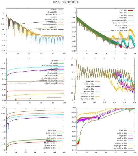
Numerical results are shown on Figure 1 (top and middle left). We use LAG17, N = 2048, vmax = 8 as default values.
use theδf method, we observe a further improvement (plots 1 to 5): we gain 4 oscillations (that is we have 27 oscillations in total) until timet= 60, and the electric field is below 6·10−6< e−12. Note that in the case where
we use theδf method, adding the zero mean modification has no impact here; on the other hand, results with theδf method are better than results with the zero mean modification on this picture. We have also added a result on an older machine (plot 9: MacBook), which leads to very poor results (only 9 oscillations until time
t= 19 for the worst method). The use of an older version of CUDA and non conforming IEEE floating point standard may explain this behaviour; this should be corrected with new versions of CUDA. Also the results, which are not shown here, due to space limitations, were different by applying the modifications; as an example, we got 28 right oscillations by using theδf method with zero mean modification. Floating point standard may not have been satisfied there which could explain the difference in the results.
In the double precision case (top right), we can go to higher precision results. By usingδf method or zero mean modification (the difference between both options is less visible), we get 92 right oscillations until time
t = 206 (the last oscillation is not good resolved hat the end), the electric field goes under 6·10−13 < e−28,
and we guess that we could add 11 more oscillations until timet= 231 (we see that grid size effects pollute the result), to obtain 103 oscillations and with electric field below 6·10−14< e−30, but we are limited here in the
double precision case to N = 2048. A CPU simulation with N = 4096 confirms the results. We also see the effect of the grid (runs withN = 1024) and the velocity (runs withvmax= 6). Note that the plot 6 (trap nodelta
1024 v6) has lost a lot of accuracy compared to the other plots: the grid size is too small (N = 1024), the velocity domain also (vmax= 6) and above all there is no zero mean orδf method. In that case, we only reach timet= 100. We refer to [17,31] for other numerical results and discussions and to the seminal famous work [23] for theoretical results. In [31], it was already mentionned that we have to take the velocity domain large enough and to take enough grid points. Concerning GPU and single precision, the benefit of a δf method was also already treated in [22]: 29 right oscillations were obtained in the single precision case with aδf modification, 13 right oscillations without the modification and the timet= 100 was reached in the CPU case (N was set to 1024 andvmax to 6).
On Figure1middle left, we plot the error of mass, which is computed as|ρ0ˆ −1|. We clearly see the impact between the conservation of the mass and the former results. We can also note that, the zero mean modification does not really improve the mass conservation (just a slight improvement at the end, plots 2,3,4), but has a benefic effect on the electric field: the bad behaviour of the mass conservation is not propagated to the electric field. On the other hand, theδfmethod clearly improves the mass conservation. We also see the effect of taking a too small velocity domain, in the double precision case.
4.2.
Bump on tail
For this second standard test case, the initial condition is considered as a spatial and periodic perturbation of two Maxwellians (see [27])
f0(x, v) =
9
10√2πexp −v 2 2 + 2
10√2πexp(−2(v−4.5) 2)
(1 + 0.03 cos(0.3x)), (x, v)∈[0,20π]×[−9,9].
The Vlasov-Poisson model preserves physical quantities with time like Casimir functions, which will be used to compare the different implementations. Particulary, we look at the time history of the total energy E of the system, which is the sum of the kinetic energyEk and the electric energyEe
E(t) =Ek(t) +Ee(t) = Z 20π
0 Z
R
f(t, x, v)v
2
2dvdx+ 1 2
Z 20π
0
E2(t, x)dx.
As in the previous case, the time evolution of the electric energy is chosen as a diagnostics. Results are shown on Figure1(middle right and bottom) and on Figure2.
3: single delta) is the winner and the basic method without modifications and trapezoidal computation of the electric field (plot 7: trap single no delta) leads to the worst result. Double precision computations lead to better results and differences are small: plots 1 (double delta) and 2 (double no delta) are undistinguishable and plot 8 (trap double no delta) is only different at the end. Thus, such modifications are not so mandatory in the double precision case. We then see for the same runs, the evolution of the error of mass (bottom left) and of the first mode of ρin absolute value (bottom right). We notice that the error of mass linearly accumulates in time. Here no error coming from the velocity domain is seen, becausevmax is large enough (vmax = 9 in all the runs). The evolution of the first mode of ρ is quite instructive: we see that it exponentially grows from round off errors and the different runs lead to quite different results. The loss of mass can become critical in the single precision case (no real impact in the double precision case are detected) and implementations without mass error accumulation would be desirable. Theδf method improves the results, but the error of mass still accumulates much more than in the double precision case.
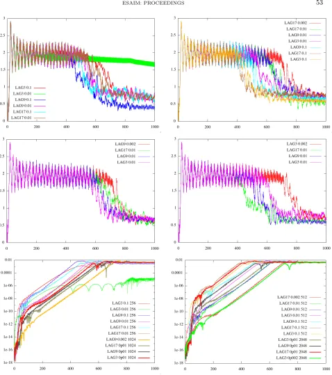
On Figure 2, we see the same diagnostics in the double precision case. We make vary the number of grid points, the degree of the interpolation and the time step. By taking smaller time step, we can increase the time before the merge of two vortices among three which leads to a breakdown of the electric field. Higher degree interpolation lead to better results (in the sense that the breakdown occurs later), for not too high grid resolution. WhenN = 2048, lower order interpolation seems to be better, since it introduces more diffusion, whereas high order schemes try to capture the small scales, which are then sharper and more difficult to deal with in the long run. Adaptive methods and methods with low round-off error in the single precision case may be helpful to get better results.
4.3.
KEEN Waves
In this last and most intricate test, instead of considering a perturbation of the initial data, we add an external driving electric fieldEapp to the Vlasov-Poisson equations:
∂tf+v∂xf+ (E−Eapp)∂vf = 0, ∂xE= Z
R
f dv−1,
whereEapp(t, x) is of the formEapp(t, x) =Emaxka(t) sin(kx−ωt), where
a(t) =0.5(tanh( t−tL
twL )−tanh( t−tR
twR ))−
1− , = 0.5(tanh(
t0−tL twL
)−tanh(t0−tR
twR ))
is the amplitude,t0= 0, tL= 69, tR = 307, twL =twR= 20, k= 0.26, ω= 0.37 andEmax= 0.2. The initial
condition is
f0(x, v) =√1
2πexp
−v 2
2
, (x, v)∈[0,2π/k]×[−6,6].
See [1,28] for details about this physical test case. Its importance stems from the fact that KEEN waves represent new non stationary multimode oscillations of nonlinear kinetic plasmas with no fluid limit and no linear limit. They are states of plasma self-organization that do not resemble the (single mode) way in which the waves are initiated. At low amplitude, they would not be able to form. KEEN waves can not exist off the dispersion curves of classical small amplitude waves unless a self-sustaining vortical structure is created in phase space, and enough particles trapped therein, to maintain the self-consistent field, long after the drive field has been turned off. For an alternate method of numerically simulating the Vlasov-Poisson system using the discontinuous Galerkin approximation, see [8] for a KEEN wave test case.
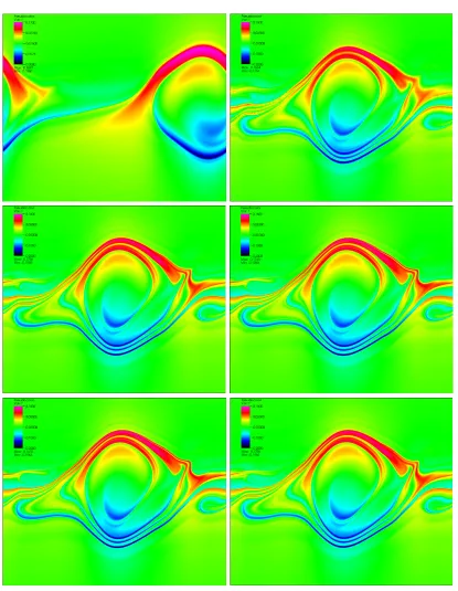
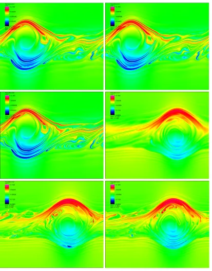
As diagnostics, we consider here different snapshots off−f0at different times: t= 200, t= 300, t= 400, t= 600 andt= 1000.
We first consider the timet= 200 (upper left in Figure3). At this time, all the snapshots are similar so we present only one (GPU single precision and a grid of 10242 points). The five others graphics of this figure are
right (GPU single precision,N= 4096 and ∆t= 0.1) is identical to the bottom left one (GPU single precision,
N = 4096 and ∆t= 0.01).
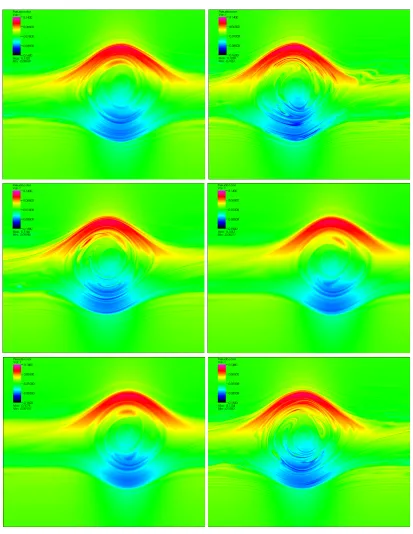
Figure4 presents different snapshots at times t= 400 andt= 600. At timet= 400, the upper left graphic (GPU single precision,N = 2048, ∆t= 0.1) is similar to the upper right one (CPU,N = 2048, ∆t= 0.05), that shows that the CPU and the GPU codes give the same results. With 4096 points (on middle left), we observe a little difference with the 2048 points case. Between the snapshots at timet= 400 and those at timet= 600, we observe the emergence of diffusion.
The time t = 1000 is considered on Figure 5. We see that there is no more convergence at this time: there is a lag, but the structure remains the same. We compare also different interpolators (cubic splines, LAG 3, LAG 9, LAG 17). If the order of the interpolation is high (graphic at the top right : CPU, LAG 17, ∆t= 0.05, Nx= 512, Nv= 4096) there is appearance of finer structures. At this time, one sees little difference between CPU results (graphic at the middle right : CPU, LAG 3, ∆t = 0.05, N = 4096) and GPU results (graphic at the bottom left : GPU, LAG 3, ∆t= 0.05, N= 4096), but there is no lag.
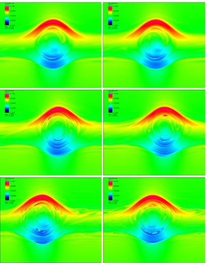
Figure 6(at time t= 1000) shows the differences between single and double precision when the value ofN
is changed. The two graphs above show the caseN = 1024, the left is single precision while the right one is in double precision. We see that there are very few differences. WhenN = 2048, the results are different in single precision (graphic on middle left) and double precision (graphic on middle right). When N = 4096, the code does not work in double precision so we compared the results for single precision GPU with ∆t= 0.05 (bottom left graphic) and ∆t = 0.01 (bottom right graphic). There are also differences due to the non-convergence. Moreover, we see that there are more filamentations whenN increases.
Figure 7 shows the time evolution of the absolute value of the first Fourier modes ofρ. We see that single precision can modify the results on the long time (top left). The GPU code is validated in double precision (top right). We clearly see the benefit of theδf method in the GPU single precision (middle left), where it has no effect in the double precision case (middle right). Further plots are given withN = 4096 (bottom left and right). With smaller time steps, some small oscillations appear with single precision GPU code (bottom right). In all the plots, we see no difference at the beginning; differences appear in the long run as it was the case for the plots of the distribution function.
4.4.
Performance results
Characteristics.We have tested the code on different computers with the following characteristics:
• GPU
– (1) = irma-gpu1 : NVIDIA GTX 470 1280 Mo; Cuda version 5.0
– (2) = hpc : GPU NVIDIA TESLA C2070; Cuda version 5.0
– (3) = MacBook : NVIDIA GeForce 9400M; Cuda version 4.2
• CPU
– (4) = MacBook : Intel Core 2 Duo 2.4 GHz
– (5) = irma-hpc2: Six-Core AMD Opteron(tm) Processor 8439 SE
– (6) = irma-gpu1: Intel Pentium Dual Core 2.2 Ghz 2Gb RAM
– (7) = MacBook : Intel Core i5 2.4 GHz
We measure in the GPU codes the proportion of FFT which consists in: transform 1D real data to complex, computing the FFT, making the complex multiplication, computing the inverse FFT, transforming to real data (together with addition of δf modification, if we use the δf method). We add a diagnostic for having the proportion of time in the cufftExec routine; we note that this extra diagnostic can modify a little the time measures (when this is the case; new measures are given in brackets, see on Table1).
The results with a CPU code (vlaso) without OpenMP are given on Table3, top; in that code, the Landau test case is run with ∆t/2 advection inx, followed by ∆t advection inv and ∆t/2 advection in xand the last advection inxof iterationnis merged with the first advection inxof iterationn+ 1.
The results with Selalib (Table 3, bottom) [26] are obtained with OpenMP. We use 2 threads for (4), 24 threads for (5), 2 threads for (6) and 4 threads for (7).
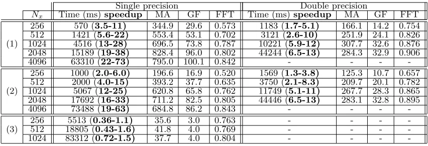
In order to compare the performances, we introduce the number MA which represents the number of millions of point advections made per second : M A = Nstep×Nadv×N2
106×Total time and the number of operations per second (in
GigaFLOPS) given by :
GF = Nstep×Nadv×(2N×5Nlog(N) + 6N
2)
109×Total time with complex data (GPU)
GF = Nstep×Nadv×(N×5Nlog(N) + 3N
2)
109×Total time with real data (CPU)
whereNsteprefers to the number of time steps andNadvrepresents the number of advections made in each time step (Nadv = 3 in GPU and Selalib codes; Nadv = 2 in vlaso code). In each advection, we compute N times (GPU in complex data) orN/2 times (CPU in real data) :
• A forward FFT and backward FFT with approximately 5Nlog(N) operations for each FFT computation
• A complex multiplication that requires 6N operations.
The speedup in Table1 and2are computed, by taking the fastest and slowest CPU simulation of Table3. The comparison between Table1 and Table2 shows that the cost of the methodδf is not too important but not negligible. This cost could be optimized. We clearly benefit of the huge acceleration of the FFT routines in GPU and we thus gain a lot to use this approach. Most of the work is on the FFT, which is optimized for CUDA in thecufftlibrary, and is transparent for the user. Note that we are limited here toN = 4096 in single precision andN = 2048 in double precision; also we use complex Fourier transform; optimized real transforms may permit to go even faster. The merge of two velocity time steps can also easily improve the speed. Higher order time splitting may be also used. Also, a better comparison with CPU parallelized codes can be envisaged (here, we used a basic OpenMP implementation which only scales for 2 processors). We can also hope to go to higher grids, sincecufftshould allow grid sizes of 128 millions elements in double precision and 64 millions in single precision (here we use 224'16.78·106elements in single precision and 222'4.2·106elements in double
precision; so we should be able to run with N = 8192 in single precision andN = 4096 in double precision). Higher complexity problems (as 4D simulations) will probably need multi-gpu which is another story, see [13] for such a work.
5.
Conclusion
We have shown that this approach works. Most of the load is carried by the FFT routine, which is optimized for CUDA in the cufft library, leading to huge speedups and is invisible to the user. Thus, the overhead of implementation time which can be quite significant in other contexts is here reduced, since we use largely built-in routines which are already optimized. The use of single precision is made harmless thanks to a δf
Single precision Double precision
Nx Time (ms) (speedup) MA FFT (cufftExec) Time (ms) (speedup) MA FFT (cufftExec)
256 703 (2.8-8.5) 279.6 0.635 (0.36) 1304(1.5-4.6) 150.7 0.767 (0.61) 512 1878 (4.3-17) 418.7 0.759 (0.46) 3516 (2.3-8.8) 223.6 0.839 (0.67) (1) 1024 6229 (9.6-20) 505.0 0.841 (0.51) 11670 (5.1-11) 269.5 0.889 (0.71) 2048 21908 (13-27) 574.3 0.861 (0.50) 49925 (5.7-12) 252.0 0.916 (0.75)
4096 90093 (15-52) 558.6 0.888 (0.54) - -
-256 1096 [1378] (1.8-5.5) 179.3 0.471 [0.59 (0.37)] 1653 (1.2-3.6) 118.9 0.637 (0.5) 512 2125 [2550] (3.8-15) 370.0 0.654 [0.69 (0.48)] 3896 (2.1-8.0) 201.8 0.777 (0.66) (2) 1024 5684 [6001] (11-22) 553.4 0.775 [0.79 (0.59)] 12127 (4.9-10) 259.3 0.866 (0.76) 2048 19871 [20284] (14-29) 633.2 0.825 (0.62) 45753 (6.3-13) 275.0 0.897 (0.80)
4096 81943 (17-57) 614.2 0.859 (0.66) - -
-256 5783 (0.3-1.0) 33.9 0.773 (0.65) - -
-(3) 512 19936 (0.4-1.6) 39.4 0.780 (0.66) - -
-1024 87685 (0.68-1.4) 35.8 0.813 (0.71) - -
-Table 1. Performance results for GPU, nbstep=1000, LAG17, KEEN wave test case withδf
modification: total time, speedup, MA, proportion FFT/total time (and cufftExec/total time).
Single precision Double precision
Nx Time (ms)speedup MA GF FFT Time (ms)speedup MA GF FFT
256 570 (3.5-11) 344.9 29.6 0.573 1183 (1.7-5.1) 166.1 14.2 0.754 512 1421 (5.6-22) 553.4 53.1 0.702 3121 (2.6-10) 251.9 24.1 0.826 (1) 1024 4516 (13-28) 696.5 73.8 0.787 10221 (5.9-12) 307.7 32.6 0.876 2048 15189 (19-38) 828.4 96.0 0.802 44244 (6.5-13) 284.3 32.9 0.906
4096 63310 (22-73) 795.0 100.1 0.842 - - -
-256 1000 (2.0-6.0) 196.6 16.9 0.520 1569 (1.3-3.8) 125.3 10.7 0.657 512 2000 (4.0-15) 393.2 37.7 0.635 3750 (2.1-8.3) 209.7 20.1 0.782 (2) 1024 5067 (12-25) 620.8 65.8 0.762 11749 (5.1-11) 267.7 28.3 0.865 2048 17692 (16-33) 711.2 82.5 0.805 44446 (6.5-13) 283.1 32.8 0.895
4096 73488 (19-63) 684.8 86.2 0.843 - - -
-256 5513 (0.36-1.1) 35.6 3.0 0.763 - - -
-(3) 512 18805 (0.43-1.6) 41.8 4.0 0.769 - - -
-1024 83312 (0.72-1.5) 37.7 4.0 0.804 - - -
-Table 2. Performance results for GPU, nbstep=1000, LAG17, KEEN wave test case without
δf modification: total time, speedup, MA, GFlops and proportion FFT/total time.
(4) (5) (6) (7)
Nx Total time MA GF Total time MA GF Total time MA GF Total time MA GF
256 4s 27.4 1.1 4s 28.8 1.2 6s 21.4 0.9 3s 38.8 1.6
512 27s 19.2 0.9 18s 28.8 1.3 31s 16.5 0.7 15s 34.7 1.6
1024 1min52s 18.7 0.9 2min4s 16.8 0.8 2min7s 16.4 0.8 1min18s 26.7 1.4 2048 8min16s 16.9 0.9 9min31s 14.6 0.8 9min42s 14.4 0.8 5min36s 24.9 1.4 4096 41min05s 13.6 0.8 48min16s 11.5 0.7 52min20s 10.6 0.6 28min28s 19.6 1.2
256 3s 58.0 2.4 4s 43.9 1.8 3s 54.3 2.3 2s 72.6 3.1
512 19s 39.6 1.9 8s 90.6 4.3 22s 35.0 1.6 13s 58.7 2.8
1024 1min25s 36.8 1.9 1min21s 38.5 2.0 1min35s 32.9 1.7 1min0s 52.1 2.7 2048 6min41s 31.3 1.8 7min46s 27.0 1.5 8min47s 28.3 1.6 4min47s 43.7 2.5 4096 34min39s 24.2 1.5 25min33s 32.8 2.0 77min31s 10.8 0.6 23min09s 36.2 2.2
Table 3. Performance results for CPU vlaso code, nbstep=1000, LAG 17, Landau test case
References
[1] B. Afeyan, K. Won, V. Savchenko, T. Johnston, A. Ghizzo, and P. Bertrand. Kinetic Electrostatic Electron Nonlinear (KEEN) Waves and their Interactions Driven by the Ponderomotive Force of Crossing Laser Beams., Proc. IFSA 2003, 213, 2003, and arXiv:1210.8105,http://arxiv.org/abs/1210.8105.
[2] T. D. Arber, R. G. Vann,A critical comparison of Eulerian-grid-based Vlasov solvers, JCP,180(2002), pp. 339-357. [3] N. Besse, M. Mehrenberger,Convergence of classes of high-order semi-lagrangian schemes for the Vlasov-Poisson system,
Mathematics of Computation, 77, 93–123 (2008).
[4] C. K. Birdsall, A. B. Langdon,Plasma Physics via Computer Simulation, Adam Hilger, 1991.
[5] K. J. Bowers, B. J. Albright, B. Bergen, L. Yin, K. J. Barker, D. J. Kerbyson, 0.374pflop/s trillion-particle kinetic
modeling of laser plasma interaction on roadrunner, Proc. of Supercomputing. IEEE Press, 2008.
[6] J. P. Boris, D. L. Book,Flux-corrected transport. I: SHASTA, a fluid transport algorithm that works, J. Comput. Phys.
11(1973), pp. 38-69.
[7] F. Charles, B. Despr´es, M. Mehrenberger,Enhanced convergence estimates for semi-lagrangian schemes Application to the Vlasov-Poisson equation,SIAM J. Numer. Anal., 51(2), 840–863 (2013).
[8] Y. Cheng, I. M. Gamba, P. J. Morrison,Study of conservation and recurrence of Runge-Kutta discontinuous Galerkin schemes for Vlasov-Poisson systems,arXiv:1209.6413v2, 17 Dec 2012,http://arxiv.org/abs/1209.6413.
[9] C. Z. Cheng, G. Knorr,The integration of the Vlasov equation in configuration space, J. Comput. Phys.22(1976), pp. 330-3351.
[10] A. Crestetto, P. Helluy,Resolution of the Vlasov-Maxwell system by PIC Discontinuous Galerkin method on GPU with OpenCL,http://hal.archives-ouvertes.fr/hal-00731021
[11] N. Crouseilles, E. Faou, M. Mehrenberger,High order Runge-Kutta-Nystr¨om splitting methods for the Vlasov-Poisson equation, inria-00633934, version 1,http://hal.inria.fr/IRMA/inria-00633934.
[12] N. Crouseilles, M. Mehrenberger, E. Sonnendr¨ucker,Conservative semi-Lagrangian schemes for Vlasov equations, J. Comput. Phys.229(2010), pp. 1927-1953.
[13] T. Dannert,GENE on Accelerators, 4th Summer school on numerical modeling for fusion, 8-12 October 2012, IPP, Garching near Munich, Germany,http://www.ipp.mpg.de/ippcms/eng/for/veranstaltungen/konferenzen/su school/.
[14] E. Fijalkow,A numerical solution to the Vlasov equation, Comput. Phys. Commun.116(1999), pp. 329-335.
[15] F. Filbet, E. Sonnendr¨ucker, P. Bertrand,Conservative numerical schemes for the Vlasov equation, J. Comput. Phys.
172(2001), pp. 166-187.
[16] F. Filbet, E. Sonnendr¨ucker,Comparison of Eulerian Vlasov solvers, Comput. Phys. Comm.151(2003), pp. 247-266. [17] F. FilbetNumerical simulations avalaible online athttp://math.univ-lyon1.fr/∼filbet/publication.html
[18] R.M. Gray,Toeplitz and circulant matrices: a review, Now Publishers Inc, Boston-Delft (2005).
[19] Y. Guclu, W. N. G. Hitchon, Szu-Yi Chen,High order semi-lagrangian methods for the kinetic description of plasmas, Plasma Science (ICOPS), 2012 Abstracts IEEE, vol., no., pp.5A-5, 8-13 July 2012, doi: 10.1109/PLASMA.2012.6383976. [20] R. Hatzky,Global electromagnetic gyrokinetic particle-in-cell simulation, 4th Summer school on numerical modelling for
fusion, 8-12 October 2012, IPP, Garching near Munich, Germany, http://www.ipp.mpg.de/ippcms/eng/for/veranstaltungen/ konferenzen/su school/.
[21] N.A. Krall, A.W. Trivelpiece,Principles of Plasma Physics, McGraw-Hill, New York (1973).
[22] G. Latu,Fine-grained parallelization of Vlasov-Poisson application on GPU, Euro-Par 2010, Parallel Processing Workshops, Springer (New York, 2011).
[23] C. Mouhot, C. Villani,On Landau damping, Acta Mathematica, volume 207, number 1, pages 29-201.
[24] J.M. Qiu, C. W. Shu,Conservative semi-Lagrangian finite difference WENO formulations with applications to the Vlasov equation, Comm. Comput. Phys.10(2011), pp 979-1000.
[25] T. M. Rocha Filho, Solving the Vlasov equation for one-dimensional models with long range interactions on a GPU, Comput. Phys. Comm. 184 Issue 1, pp. 34-39 (2013).
[26] Selalib, a semi-Lagrangian library,http://selalib.gforge.inria.fr/
[27] M. Shoucri,Nonlinear evolution of the bump-on-tail instability, Phys. Fluids22(1979), pp. 2038-2039.
[28] E. Sonnendr¨ucker , N. Crouseilles , B. Afeyan,BP8.00057: High Order Vlasov Solvers for the Simulation of KEEN Wave Including the L-B and F-P Collision Models, 54th Annual Meeting of the APS Division of Plasma Physics Volume 57, Number 12, Monday-Friday, October 29–November 2 2012; Providence, Rhode Island,http://meeting.aps.org/Meeting/ DPP12/SessionIndex2/?SessionEventID=181483.
[29] E. Sonnendr¨ucker, Approximation num´erique des ´equations de Vlasov-Maxwell, Master lectures, http://www-irma. u-strasbg.fr/∼sonnen/polyM2VM2010.pdf.
[30] G. Stantchev, W. Dorland, N. Gumerov,Fast parallel particle-to-grid interpolation for plasma PIC simulations on the GPU, J. Parallel Distrib. Comput.,68(10), pp. 1339-1349, (2008).
Figure 1. Linear Landau damping. N = 2048, ∆t = 0.1,vmax = 8, LAG17, irma-gpu1 on
GPU as default. Evolution in time of electric energy in single/double precision (top left/right). Error of mass |ρ0ˆ −1| with single precision as default (middle left). Bump on tail test case.
Figure 3. KEEN wave test case (LAG17): f(t, x, v)−f0(x, v). At timet= 200, GPU single precisionN = 1024 (top left). At timet= 300, GPU single precisionN = 1024,2048,4096 and ∆t = 0.1 (top right, middle left, middle right). N = 4096 and ∆t= 0.01 (bottom left). CPU
Figure 4. KEEN wave test case (LAG17): f(t, x, v)−f0(x, v). At timet= 400, GPU single precision N = 2048,∆t = 0.1 (top left). CPU ∆t = 0.05 (top right). GPU single precision
Figure 7. KEEN wave test case (LAG17): Absolute values of the first Fourier modes of ρ (from mode k = 1 to mode k = 7) vs time. δf method, with N = 2048 ∆t = 0.05 GPU, double and single precision (1b,2b,3b) (top left). double GPU and double CPU (top right). Full version GPU in single precision and δf version CPU (middle left). Full version and δf