S. Descombes, B. Dussoubs, S. Faure, L. Gouarin, V. Louvet, M. Massot, V. Miele, Editors
MACROSCOPIC MODELIZATION OF THE CLOUD ELASTICITY
∗J.-M. Etancelin
1, S. Faure
2, T. Fevrier
3et C. Huynh
4R´esum´e. La gestion des ressources informatiques `a la demande est une caract´eristique propre `a l’in-formatique en nuage. Pour que cela devienne une r´ealit´e, les fournisseurs de solutions en nuage ont besoin d’un mod`ele math´ematique leur permettant de simuler l’allumage et l’extinction des ressources en fonction de la demande. Cet article propose une premi`ere ´etape de mod´elisation bas´ee sur des outils issus de la simulation d’´ecoulements de fluides. D’une part, nous traiterons la question du temps de service dans l’optique de satisfaire simultan´ement les contraintes du fournisseur et du client. D’autre part, nous compl`eterons le mod`ele afin de simuler un comportement ´elastique des ressources du nuage. Ce comportement sera ´etabli en temps r´eel et en fonction des demandes ´eventuellement concurrentes des clients. Nous int´egrerons ´egalement au mod`ele des m´ecanismes utilis´es en pratique dans les ser-veurs comme l’arrˆet de requˆetes trop longues. Ces probl´ematiques seront illustr´ees par des simulations num´eriques men´ees `a l’aide d’un sch´ema volume fini implicite.
Abstract. In order to achieve its promise of providing information technologies (IT) on demand, cloud computing needs to rely on a mathematical model capable of directing IT on and off according to a demand pattern to provide a true elasticity. This article provides a first method to reach this goal using a “fluid type” partial differential equations model. On the one hand it examines the question of service time optimization for the simultaneous satisfaction of the cloud consumer and provider. On the other hand it tries to model a way to deliver resources according to the real time capacity of the cloud that depends on parameters such as burst requests and application timeouts. All these questions are illustrated via an implicit finite volume scheme.
Introduction
Is it necessary to define Cloud computing since it is heard and overheard? Cloud computing is about revolutionizing the Information Technology (IT) consumption behavior without questioning the underlying technologies, be it applications or infrastructure. Cloud computing is about doing more business with less i.e. fewer infrastructures (servers, network, and storage) and less effort (self service portal, orchestration).
It is important to notice that Cloud computing is enduring an inflection point; it’s all about shared elastic capabilities [4]. Let’s quote a Gartner’s analysis that is often reflected in reality: “Vendors across many
∗This work was supported in part by AMIES (http://www.agence-maths-entreprises.fr)
and by the GDR CNRS Math´ematiques et Entreprises (http://www.maths-entreprises.fr)
1 Laboratoire Jean Kuntzmann, Universit´e Joseph Fourier, Grenoble, France. Mail :[email protected] 2 CNRS, Laboratoire de Math´ematiques d’Orsay, Universit´e Paris-Sud, Bˆatiment 425, 91405 Orsay Cedex, France.
Mail :[email protected]
3 Laboratoire de Math´ematiques d’Orsay, Universit´e Paris-Sud, Bˆatiment 425, 91405 Orsay Cedex, France. Mail :[email protected]
4 Cisco Systems France, L’Atlantis, 11 rue Camille Desmoulins 92782 Issy les Moulineaux, France. Mail :[email protected] c
EDP Sciences, SMAI 2013
categories have grabbed the term and use it for marketing purposes. Hosting solutions that have a pay-per-user-per-month pricing model, but without shared elastic capabilities, are being called cloud. As cloud is used to apply to an ever-widening set of external services without regard to sharing, elasticity and the other characteristics that set cloud apart, the term becomes even more unclear. Companies may buy these cloud services and then be surprised to find that they do not get the agility and cost savings promised by cloud computing. This has pushed cloud toward the Trough of Disillusionment.” [5]
A first solution is a deal where each cloud consumer subscribes for a given amount of resources (number of virtual machines, network, and storage) and has a means of manually tune up and down consumption according to spotted demands. Such solution assumes that cloud consumers know exactly and timely what their needs may be. Unfortunately, reality check tends to prove the opposite: cloud consumer candidates are used to own IT resources and ignore completely how they are really used.
Our challenge is to fill the gap with a quantitative analysis. What if IT resources can be provisioned and deprovisioned automatically using a small set of variables, such as Service Level Agreement (SLA), reserved resource, elasticity ratio, total resource pool size?
Unlike some research, not any assumption on application type is made. Our model is designed to be attractive to as many cloud providers as possible. There is no use of consumer behavior statistics, since our model has to be applicable to local cloud providers who do not have the same range of IT resources than Google, Amazon, and the likes.
SLA is narrowed to two values: upper and lower watermarks on the service time. It’s tempting to reflect a more sophisticated model. However, the simpler is the model, the faster cloud provider will implement. The upper watermark is the maximum delay a cloud consumer may tolerate. Above this limit, a cloud consumer expects his counterpart to activate elasticity to absorb pressure. The lower watermark is the minimum delay a consumer is ready to pay for. Under this limit, a cloud consumer expects his counterpart to save costs by deprovisioning IT resources.
Reserved resource is an amount of IT elements that a cloud subscriber deems necessary to have permanently, no matter it is used or idle. Elasticity ratio is a number of IT resources that is provisioned and deprovisioned according to temporary needs. The total resource pool size is the total capacity set by a cloud provider. It is the sum of all reserved pools and the elasticity pool shared among all cloud consumers.
First, the model from Jaisson and de Vuyst is exposed and adjusted to the cloud context. Second, a mechanism is added to satisfy upper and lower service bounds. It consists in the optimization of a cost function. This allows us to handle concurrent requests in the cloud. A model considering the drop of requests when the server is saturated is also implemented. The last part is devoted to use our tool in order to attribute a first IT set to a consumer according to his forecast of consumption.
1.
Adjustment of Jaisson-de Vuyst model to the cloud
1.1.
Description of the initial model
The following model for multithreads systems has been developed by Jaisson and De Vuyst [3]. It mimics the fluid flow behavior in a macroscopic way. Indeed, microscopic models become irrelevant when big amounts of data have to be scheduled and the cloud purpose is to fill up the virtual machines (VM) constituting it of requests to treat a lot of data. Moreover, it introduces a space variable to take into account memory and de-lay features of the transport of information. In the following, we reuse Jaisson’s and De Vuyst’s notations, see [3].
and then the total massm(t) of requests in the system :
m(t) =
Z 1
0
ρ(x, t)dx. (1)
The input rate of requests is denoted byφi.
To derive the model equations, a mass balance is written. The variation of the current mass of requests being processed between two levels of completionwlandwris the difference between the entering flux atwland the leaving flux at wr:
d dt
Z wr
wl
ρ(x, t)dx=ρ(wl, t)φo
m(t) −
ρ(wr, t)φo
m(t) . (2)
Makingwrtend to wl in (2) gives the following Partial Differential Equations (PDE):
∂tρ+v(t)∂xρ= 0, x∈]0,1[, t >0,
v(t) = φo
m(t).
However this transport equation allows the velocity,v(t), to tend to infinity when the mass goes to zero that is physically impossible. That’s why a limiter is used to have a maximal velocity equal to the system capacity
φo:
v(t) = φo max(1, m(t)).
The integration of the transport equation on space gives a mass conservation Ordinary Differential Equation (ODE). To complete the model, initial conditions att= 0 on the flux and the mass and a boundary condition atx= 0 (input flux) are added. It comes:
∂tρ+v(t)∂xρ= 0, x∈]0,1[, t >0, (3a)
∂tm=φi(t)−ρ(1, t)v(t), t >0, (3b)
v(t) = φo
max(1, m(t)), (3c)
ρ(x,0) =ρ0(x), (3d)
m(0) =
Z 1
0
ρ0(x)dx≥0, (3e)
ρ(0, t)v(t) =φi(t). (3f)
In the context of the cloud, the evaluation of the service time of the system is an important issue. We denote byd(x, t0, x0) the time for a request to be completed at levelxgiven that it was at levelx0 at timet0. So the
whole service time of a task at timetis defined by D(t) =d(1, t,0) anddis transported at the velocity v(t):
∂td+v(t)∂xd= 1, x∈]0,1[, t >0, (4a)
d(0, t,0) = 0. (4b)
A change of variableu=t−din (4) gives the following homogeneous system over service time:
∂tu+v(t)∂xu= 0, x∈]0,1[, t >0, (5a)
u(0, t) =t, (5b)
The quantity of interest,D(t), is computed by solving simultaneously the two systems of equations (3) and (5) with the numerical scheme detailed in section 1.3.
1.2.
Adjustment to the cloud
The cloud is made of an initial set of virtual machines (VM) which can be allocated on demand to cloud consumers. Each customer subscribes to a number of VM for a certain duration, typically a year, usually three years. Resignation can happen at any time (its obtention is explained later in Section 2.4). This number corre-sponds to a certain capacityφowhich belongs to the cloud consumer. Once assigned to a consumer, a VM is no longer available nor accessible to other clients. It is called multi-tenancy and implies that cloud consumers share the resources provided by the cloud provider with all the required confidentiality, integrity, and availability levels.
As a consequence, to each cloud user corresponds one system as above with its own capacityφoand its own set of equations to solve: systems (3) and (5). There are as many independent systems as cloud consumers, since there are no communication between them. There are also a pool of unassigned VM that a cloud user may request according to its SLA and cloud provider commitment to elasticity (see Section 2.2). Without any client, the pool may be the whole capacity of the cloud provider. As clients keep coming, the pool size decreases, unless the cloud provider refills it by adding extra capacity.
In Section 2.3 the model will be enriched in order to integrate the possibility for the VM to drop requests when the service time is too long. It reproduces the usual behavior of servers for timeout requests.
1.3.
Numerical scheme
Following [2], the system (3)-(5) is solved by a Finite Volume method (see for example [1]). The domain [0; 1] is discretized by N control volumes defined by [xj−1
2;xj+12] where xj+21 =jh, j ∈ {0, . . . , N} and h= 1/N.
The cells centers are the pointsxj= (j−1/2)h, j∈ {1, . . . , N}.
The time discretization is ensured by an upwind implicit scheme with a time stepdtnwhich is unconditionally stable and can be solved explicitly. Hence, forj ∈ {1, . . . , N}, the unknowns are meant to be approximations of the cell averages withtn =tn−1+dtn forn= 1, . . . , N
t andt0= 0:
ρnj = 1
h Z xj+ 1
2
xj−1 2
ρ(x, tn)dx, (6)
mnj = 1
h Z xj+ 1
2
x j−1
2
m(x, tn)dx, (7)
unj =tn− 1
h Z xj+ 1
2
xj−1 2
Using the above notations, the full discretization of the system (3)-(5) is given by the following scheme, with
λn=dtn/h:
vn = φo
max(1, mn), (9a)
ρn1+1=ρn1 −λn(ρ
n+1 1 v
n−φn+1
i ), (9b)
ρjn+1=ρnj −λn(ρjn+1−ρnj−+11)vn, (9c)
mn+1=mn+dtn(φin+1−ρnN+1vn), (9d)
un1+1=tn+1, (9e)
unj+1=unj −λn(u n+1
j −u n+1
j−1)v
n, (9f)
Dn+1=tn+1−unN+1. (9g)
1.4.
Numerical validation
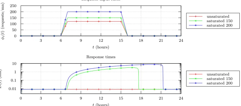
The model is validated choosing different input request rates. In the following, we consider a 24 hour simulation with a time discretization of 1 minute (i.e. 1,440 time-steps). For the spatial discretization, 1,000 grid points are considered. The cloud consumer is using a cloud resource capacity of 120 requests per time-step. On Figure 1, the three input rates considered present a plateau of height 120, 150 and 200 requests per time-steps between 6 and 16 hours. In the first case, the system can process the whole input at its maximum speed whereas, for the others, the system is saturated and the service time increases. One can note that the bigger the amount of saturating requests is, the longer the service time takes to fall back to decent.
0 50 100 150 200 250
0 3 6 9 12 15 18 21 24
φi
(
t
)
(requests/mn)
t(hours) Requests input rates
unsaturated saturated 150 saturated 200
0.01 0.1 1 10
0 3 6 9 12 15 18 21 24
D
(
t
)
(mn)
t(hours) Response times
unsaturated saturated 150 saturated 200
2.
Service time optimization
2.1.
The cost function
The easiest way to control the service time is to adjust the amount of resources allocated to a cloud consumer. In fact this time varies with the number of VMS and their computational characteristics. In our model, it means to varyφo.
As service time is a key quantity in networks, several optimizations can be done. From an end-user point of view, the service time should not be higher than a given time denotedTmax. For the cloud provider, it must be greater thanTmin in order to prevent quality overachievement and keep resources available for incoming cloud consumers. These bounds over the service time depend on each kind of requests. For example, for a basic web service we could chooseTmax= 3 seconds andTmin= 0.1 seconds. For data archiving, it could be respectively 6 hours and 1 hour.
In the real life, there is no means for a cloud provider to predict the requests input rate. The best that one can do is to monitor it. Therefore, optimizations are performed at a certain frequency, depending on the kind of service. Requests are supposedly independent, most of the time. Things may change when customer gets angry and retries the same request over and over again. We are interested in controlling the service time over small time windows of length ∆t, regarding last input data available (such an assumption relates to the most of applications eligible to the cloud). We search for an optimal capacityφ∗o∈]0;φo] over ∆ttime windows with the minimization of the following cost function:
Jn(φ∗o) =
Z tn+∆t
tn
(D(t, φ∗o)−Tmin)2+ (D(t, φ∗o)−Tmax)2dt. (10)
We denote byφ∗n
o the capacity that realizes:
Jn(φ∗on) = Min φ∗
o∈]0;φo]
Jn(φ∗o). (11)
Therefore, the evolution of the optimal capacity for a cloud consumer is defined by a time dependent piecewise constant functionφ∗o(t):
φ∗o(t) =φ∗on ift∈]tn;tn+1].
However switching on or switching off VM takes a certain time. So modifying capacity is not instantaneous. That is the reason why we introduce a delay δt before applying the optimal capacity. This optimal capacity function becomes:
φ∗o(t) =φ∗on ift∈]tn+δt;tn+1+δt]. (12)
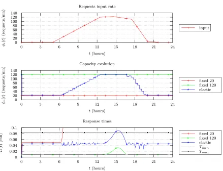
The capacity optimization influence can be observed on Figure 2. The service time is computed for three cloud consumers with identical inputs. One of them has his capacity optimized to haveD(t)∈ [0.5; 5]. In the first case, the client is running a constant low capacity and sees his service time exploding at t= 6 hours. In the second case, he is using all his VM and then obtains a constant low service time except at t = 15 hours where his system is lightly saturated. Finally, in the last case, optimization is performed every 20 minutes, the cloud consumer uses the elasticity of the cloud. One can observe that the service time is correctly placed between the bounds, the capacity is reduced when the input is quite low and increased when it is necessary. We have therefore the evidence that there is no need to commit to a too low service time and both client and cloud provider are better off switching off VM when they don’t use them.
2.2.
Generalization to many cloud consumers
In a cloud, each consumer is allocated a set of VM of capacityφo he is the only one to use (part 1.2). So a part of size P
c∈clients
φo,cof the cloud is fixed. If we denote by Φ the whole capacity of the cloud, Φ− P c∈clients
φo,c
0 20 40 60 80 100 120 140
0 3 6 9 12 15 18 21 24
φi
(
t
)
(requests/mn)
t(hours) Requests input rate
input
0 20 40 60 80 100 120 140
0 3 6 9 12 15 18 21 24
φo
(
t
)
(requests/mn)
t(hours) Capacity evolution
fixed20
fixed120
elastic
0 0.02 0.04 0.06 0.08 0.1
0 3 6 9 12 15 18 21 24
D
(
t
)
(mn)
t(hours) Response times
fixed20
fixed120
elastic
Tmin Tmax
Figure 2. Capacity optimization influence.
cloud consumers according to the extra capacity they have bought and to the unassigned shared pool of the cloud.
Two things have to be defined: what part they can catch and when they need more capacity. For the first matter, each cloud user chooses and buys an option to use his extra capacity rate defined byφeo∈[0,1]. Thus if a cloud consumer has an allocated capacity ofφohe can use a maximum ofφo(1 +φeo). It is considered that he needs this extra capacity at timetn if he is already using more thanφ
o which means thatφ∗on>φo.
Lettnbe the present time. Cloud consumers are ordered by decreasing service time. Thus the most saturated are served in priority. If a client uses less thanφo (ie ifφ∗on< φo), he does not need any extra capacity. SoJ is minimized on ]0;φo]. Otherwise (i.e. φ∗on >φo) he is allowed to use extra-resources. Nevertheless, the cloud provider can not always deliver him the whole φeo. Indeed, he can not provide more than the remaining free resources in the cloud. As in section 2.1, one can define the available capacity by a piecewise function:
φnav= Φ− X
c∈clients
φ∗o,cn. (13)
So if φn
φo(1 +φeo)−φ∗on≤φnav, J is optimized on ]0;φo(1 +φeo)], else it is optimized on ]0;φ∗on+φnav].
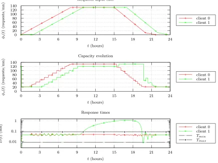
An illustration of this algorithm is presented on Figure 3: there are two cloud consumers in the cloud. Each one owns a capacity of 120 and a free set a of capacity 12 is available. Both are authorized to take at most an extra capacity of 10% of their initial set (132). Clients don’t have any reason to share the same numbers (120, 12, 10%) and the logic remains beyond 2 clients. Numbers are chosen for the sake of simplicity and clarity in the graphs. The same input (with a maximum of 132 requests per time-step) is launched by both, slightly before for the first client. As a consequence, he is the first to need an extra capacity: he takes all the available VM to satisfy his 10%. This relieves his service time which evolves in the expected interval. The second client becomes saturated later but no extra capacity is available until 16 hours. During this period, his service time grows and overpasses the upper bound. At 16 hours, the first consumer releases his extra capacity because of his input decrease. Thus the second one can take his 10% and stabilize his service time.
0 20 40 60 80 100 120 140
0 3 6 9 12 15 18 21 24
φi
(
t
)
(requests/mn)
t(hours) Requests input rate
client 0 client 1
0 20 40 60 80 100 120 140
0 3 6 9 12 15 18 21 24
φo
(
t
)
(requests/mn)
t(hours) Capacity evolution
client 0 client 1
0.01 0.1 1
0 3 6 9 12 15 18 21 24
D
(
t
)
(mn)
t(hours) Response times
client 0 client 1
Tmin Tmax
Figure 3. Two semi-shared ressources cloud consumers.
2.3.
Add request cessation in the model
In this section, we integrate to our model a mechanism that lighten the servers workload: when the service time overpasses a certain threshold, the cloud must stop a chosen rate of requests.
Let’s noteτ(t) the damping of requests transport andTththe threshold. It is assumed that the damping is uniform over the completion rate. Letτ(t) be equal to 0 whenD(t)≤Tthand be a positive constant elsewhere. To model this suspension phenomenon, an additional term appears in the mass balance (2) representing the part of the deleted mass betweenwland wr:
d dt
Z wr
wl
ρ(x, t)dx= ρ(wl, t)φo
m(t) −
ρ(wr, t)φo m(t) −τ(t)
Z wr
wl
ρ(x, t)dx.
The flux equation becomes:
∂tρ+v(t)∂xρ=−τ(t)ρ(x, t), x∈]0,1[, t >0, (14)
v(t) = φo
max(1, m(t)). (15)
(16)
The requests density is still transported with the same velocityvbut a damping factor when the service time is too high is added as a source term. Integrating this equation in space, the mass ODE reads
∂tm=φi(t)−ρ(1, t)v(t)−τ(t)m(t), t >0. (17)
Regarding the numerical scheme, these new terms are treated implicitly.
We show the damping influence on Figure 4 where a cloud consumer is handled with different values for τ. The first case corresponds to previous results with no requests dropping. As one can see, the amount of input requests makes the client saturated between 12 and 19 hours. The use of requests cessation makes the service time below the threshold time Tth during the saturation period. It decreases as strong asτ is high. We notice also that as much asτ is increasing, the system needs less and less drops.
2.4.
Cloud consumer resources dimensioning
When a consumer subscribes to the cloud, he chooses different types of applications. These applications can be translated in an equivalent number of requests per time-step and more precisely in a forecasting of input for a certain time sample. Note that the real input can be different from this forecasting. The client may not know exactly what resources amount he needs for his applications, so we could use the model as a sizing tool.
First we assume that there is one cloud consumer to size in the cloud. As it is explained above, with his subscription, the client provides an estimation of the future input. The idea is to launch the optimization algo-rithm on this forecasting input, the first φo being fixed to the total available cloud resources. The simulation gives a capacity profile from which we extract the maximum of capacity we propose to the client as the capacity he needs to handle his requests.
0 20 40 60 80 100 120 140
0 3 6 9 12 15 18 21 24
φi ( t ) (requests/mn) t(hours) Requests input rate
input 0 20 40 60 80 100 120 140
0 3 6 9 12 15 18 21 24
φo ( t ) (requests/mn) t(hours) Capacity evolution
τ= 0
τ= 1
τ= 10
τ= 100
τ= 1000
0.1 1 10 100 1000
0 3 6 9 12 15 18 21 24
τ ( t ) t(hours) Drop rates
τ= 1
τ= 10
τ= 100
τ= 1000
0.01 0.1
0 3 6 9 12 15 18 21 24
D ( t ) (mn) t(hours) Response times
τ= 0
τ= 1
τ= 10
τ= 100
τ= 1000
Tmin Tmax Tth
Figure 4. Influence of request cessation,Tth= 3Tmax.
Conclusion
should be tested on real data sets. Some improvements could also be made with the addition of a variance term on capacity in the functional to prevent the excess of capacity oscillations.
References
[1] R. Eymard, T. Gallou¨et, and R. Herbin. Finite volume methods. InHandbook of numerical analysis, Vol. VII, Handb. Numer. Anal., VII, pages 713–1020. North-Holland, Amsterdam, 2000.
[2] P. Jaisson. Syst`emes complexes gouvern´es par des flux: sch´emas de volumes finis hybrides et optimisation num´erique. PhD thesis, ´Ecole Centrale Paris, 2006.
[3] P. Jaisson and F.D. Vuyst. An innovating pde model based on fluid flow paradigm for multithread systems.Computer Networks, 52(18):3318–3324, 2008.
[4] M. Kuperberg, N. Herbst, J.V. Kistowski, and R. Reussner. Defining and quantifying elasticity of resources in cloud computing and scalable platforms.Karlsruhe Reports in Informatics, 16, 2011.