Please cite this article as: R.ParviziMoghadam, F.Shahraki, J.Sadeghi, Online Monitoring for Industrial Processes Quality Control Using Time Varying Parameter Model,International Journal of Engineering (IJE),IJE TRANSACTIONS A: Basics Vol. 31, No. 4, (April 2018) 524-532
International Journal of Engineering
J o u r n a l H o m e p a g e : w w w . i j e . i rOnline Monitoring for Industrial Processes Quality Control Using Time Varying
Parameter Model
R. Parvizi Moghadam, F. Shahraki*, J. Sadeghi
Center for Process Integration and Control (CPIC), Department of Chemical Engineering, University of Sistan and Baluchestan, Zahedan, Iran
P A P E R I N F O
Paper history:
Received 22 November2017
Received in revised form 31 December2017 Accepted 04 Januray2018
Keywords: Soft Sensor
Time Varying Parameter SRU
Quality Estimation Identification Data- based Modeling
A B S T R A C T
A novel data-driven soft sensor is designed for online product quality prediction and control performance modification in industrial units. A combined approach of time variable parameter (TVP) model, dynamic auto regressive exogenous variable (DARX) algorithm, nonlinear correlation analysis and criterion-based elimination method is introduced in this work. The soft sensor performance validation is tested by data set of an industrial SRU. The comparative study indicated the result associated with more robust soft sensor and more appropriate performance index values compared to other methods for SRU soft sensor design in diverse achievements. Due to high prediction accuracy, the low complication of the model and also saving of time, this technique can be very noticeable in industrial processes control.
doi: 10.5829/ije.2018.31.04a.02
1. INTRODUCTION1
In the recent decades, the process control and monitoring have been affected by modern control methods. Due to high importance of some key variables that are hardly measurable in divers’ processes, it is indispensable the use of new techniques with high precision. With this approach, one can overcome to time wasting and several major problems caused by process of non-linearity and multivariate nature [1, 2]. In modern control, there is a valuable technology based on mathematical model and process technological knowledge under name of “soft sensor” that is veryless costly compared to expensive hardware sensors. Also, it can be a good alternative technology work in parallel. Furthermore, the soft sensors can introduce as algorithms that resolve the control problems related to variables are hardly measurable through variables which are easily measurable [1, 3]. The new versions of soft sensors in addition to monitoring and process control can apply for key variable prediction from process data measurements. Off-line lab analysis or data achieved from GC have higher financial burden for control process and soft sensor can reduce these costs [4].
*Corresponding Author Email: fshahraki@eng.usb.ac.ir (F. Shahraki)
Two classes of soft sensors based on process model or process data are defined and also, there is a hybrid model being a combination of two mentioned types consisting of fundamental process knowledge and process inputs and outputs data [5].
inputs and outputs data are useful in process control [15]. Locally weighted regression (LWR) compared to ANN led to fewer complexes linear model, by pre-processing algorithms [16]. Also, it should be noted that some of ANN models such as multi-layer perceptron (MLP) by applying pre-processing algorithm can solve problems caused by missing value and outliers [17, 18]. Another difficulty about ANN is the problems with the approximation of networks appropriate topology [4]. Categorizing the process state into the local data subsets, which is able to identify both time-varying characteristics and process nonlinearity situations can be introduced. Another method for soft sensor modeling that is Just-in-time learning (JITL) [19, 20]. But to remove the problems caused by the correlation between the process variables, the correlation-based on just-in-time learning (CoJIT) method can be more desirable [21]. Despite the above mentioned, sometimes an unfit model conformity from the relation between data sets may be obtained [22, 23]. Extended Kalman filter (EKF) algorithm is widely used as analytical approximation observer and online estimator that by the first-order linearization in a nonlinear system, distributes the parameters [24, 25]. Dual Extended Kalman filter (DEKF) is a modified form of EKF that can estimate the parameters and states of the process. It is very appropriate algorithm related to data-based systems and identification manners [26]. The data-based mechanistic (DBM) with the recorded data availability extending in the industrial process and computational power attracted more and more interest of researchers to test the method [4, 27-30].
This paper introduces a new DBM approach for soft sensor design in sulfur recovery unit (SRU) that is appropriate for dynamic systems modeling. This soft sensor is based on recorded data and DARX model (some time series algorithms such as recursive KF that predict and update the process state vector and parameters and yield the optimum parameters). The nonlinear correlation analysis and criterion-based elimination integrated by “CAPTAIN” toolbox that is successfully utilized and developed in recent decades, at Lancaster University. The model prediction capability is evaluated by missing data existence in observed industrial data and also by comparison with diverse methods.
2. PRELIMINARIES
2. 1. Data- based Mechanistic (DBM) Description In this approach, the TVP and or state dependent parameters (SDP) methods are applied for stochastic models identification and estimation in diverse non-linear and non- stationary processes. To achieve the mentioned algorithms in DBM, unobserved components (UC) stochastic state-space formulation, the recursive Kalman filter (KF) and also fixed interval smoothing
(FIS) algorithms are required. The construction of TVP regression model is commonly applied [31]. The final parameters estimation step of non-linear modeling relying on Gaussian suppositions, is performed by least squares or maximum likelihood (ML) estimation as non-linear optimization methods [32].
2. 2. State Space Model Structure It is essential to consider some assumptions for TVP related to their temporal variation situation. The observation and states equations in the state space can be constructed by:
Equation of observation: 𝑦𝑡= 𝐻𝑡𝑥𝑡+ 𝑒𝑡 (1)
Equation of state: 𝑥𝑡= 𝐹𝑥𝑡−1+ 𝐺𝜂𝑡 (2)
𝑥𝑡= [𝑥1,𝑡𝑇𝑥1,𝑡𝑇 … 𝑥𝑛+𝑚+1,𝑡𝑇 ]𝑇 (3)
𝐻𝑡= [−𝑦𝑡−1 0 − 𝑦𝑡−2 0 … −
𝑦𝑡−𝑛 0 𝑢𝑡−𝛿 0 … 𝑢𝑡−𝛿−𝑚 0]
(4)
𝑦𝑡 ,𝑥𝑡 ,𝑒𝑡and 𝜂𝑡 are the scalar stochastic observed
variable, the stochastic state variables, observation noise and white noise of input vectors, respectively. Furthermore, in state space models (n+m+1) is the parameters number and if p= 2(n+m+1), 𝐻𝑡 is a 1×p
vector that refers to the relation between scalar observation 𝑦𝑡 and the state variables in the model.
Generalized random walk (GRW) model is applied for each 𝑥𝑖,𝑡 stochastic assessment and it is defined in the
state space term and dimensions of F and G are p×p block diagonal matrixes that 𝐹𝑖 and 𝐺𝑖 matrices are given by:
𝑥𝑖,𝑡= 𝐹𝑖𝑥𝑖,𝑡−1+ 𝐺𝑖𝜂𝑖,𝑡i= 1, 2 , …, n+m+1
(5) 𝐹𝑖= [𝛼 𝛽
0 𝛾] ; 𝐺𝑖= [ 𝛿 0
0 𝜀]; 𝜂𝑖,𝑡= [𝜂1𝑖,𝑡𝜂2𝑖,𝑡] 𝑇
Also, 𝜂𝑖,𝑡 is considered to be described by a normally
diagonal covariance matrix 𝑄𝜂𝑖. The constant parameters
in above model (𝛼, β , 𝛾, 𝛿, 𝜀 ) are introduced as hyper-parameters, and depend on different cases such as: integrated random walk (IRW), scalar random walk (RW), smoothed random walk (SRW), first-order autoregressive process (AR(1)), local linear trend (LLT) and damped trend (DT). The normally constants 𝛼, β , 𝛾, 𝛿 and 𝜀 are diverse from others [33, 34]. In the present model, the IRW is applied (𝛼= β = 𝛾=𝜀 = 1; δ=0).
2. 3. TVP Models Identification The GRW model, with implementation of recursive FIS is one of the best known methods which is significantly used in chemical industry non-stationary processes such as distillation columns for parameters estimation. The FIS algorithm is constructed to estimate the time varying parameters.
pass filtering” and “backward pass smoothing” algorithms by the implementation of the KF concepts and the data in temporal order. The KF equations provide the optimal state vector reconstruction. They are consisting observations prediction equations, the state variables propagation and correction equations for updating the state estimates. The possibility to handle missing observations has fulfilled by separation of the prediction formulas and state estimation formulas [35]. The equation of TVP model can be presented in the regression vector form:
𝑦𝑡= 𝑧𝑡𝑇𝑝𝑡+ 𝑒𝑡 ; 𝑒𝑡~𝑁{0, 𝜎2} ;t=1, 2, …, N (6)
where, 𝑒𝑡 is the white noise and 𝑧𝑡𝑇 as the model states
vector and 𝑝𝑡 as the model parameters vector are given
by:
𝑧𝑡𝑇= [ 𝑦𝑡−1 𝑦𝑡−2… 𝑦𝑡−𝑛𝑢𝑡−𝛿… 𝑢𝑡−𝛿−𝑚 ]
(7) 𝑝𝑡= [ −𝑎1,𝑡 − 𝑎2,𝑡 … − 𝑎𝑛,𝑡𝑏0,𝑡… 𝑏𝑚,𝑡 ]𝑇
Regression model structure of TVP including dynamic linear regression (DLR), dynamic auto regression (DAR) and dynamic auto-regressive with exogenous variable (DARX) model are applied in most cases. The DLR as the simplest one that yet is widely used in the formulation can be described by:
𝑦𝑡= ∑𝑖=1𝑖=𝑚𝑏𝑖,𝑡𝑢𝑖,𝑡+ 𝑒𝑡; 𝑒𝑡~𝑁{0, 𝜎2} ; t=1,…,N (8)
Where bi,t, ui,t , and yt are constant parameters, regressors
and a dependent variable, respectively. The output series past values in DAR model are introduced as input variables. This is given by:
𝑦𝑡= −𝑎1,𝑡𝑦𝑡−1− 𝑎2,𝑡𝑦𝑡−2− ⋯ − 𝑎𝑛,𝑡𝑦𝑡−𝑛+ 𝑒𝑡 (9)
2. 3. 1. The DARX Model The DARX model can be used for analysis of the exact dynamic system and non-stationary time series. In this model consider the time delay for both input and output variables. The following equation can describe the case of output variable yt and
an input variable ut presence:
𝑦𝑡= −𝑎1,𝑡𝑦𝑡−1− 𝑎2,𝑡𝑦𝑡−2− ⋯ − 𝑎𝑛,𝑡𝑦𝑡−𝑛+
𝑏0,𝑡𝑢𝑡+ 𝑏1,𝑡𝑢𝑡−1+ ⋯ + 𝑏0,𝑡𝑢𝑡− 𝑛 + 𝑒𝑡 (10)
In actual, a particular instance of the discrete-time transfer function (TF) model can be described by DARX model that obtained from algorithms of least squares-based recursive filtering and the following form:
𝑦𝑡=𝐵(𝑍
−1,𝑡)
𝐴(𝑍−1,𝑡)𝑢𝑡+
1
𝐴(𝑍−1,𝑡)𝑒𝑡 (11)
That A(z-1,t) = 1+ a
1,t z-1 + … + an,t z-n is the denominator
polynomial of TF model and B(z-1,t) = b
0,t + … + bn,t z-n
is nominator polynomials which the regressors backward shift operator shows by z-r. Also, for the convenience of
writing, do not consider time delay and polynomials order similar to equation (3) [36].
2. 3. 2. Forward-pass Recursive Least Square Filtering The algorithm form of recursive least square filtering for the time series has demonstrated by:
1. Equation of prediction:
𝑥̂𝑡|𝑡−1= 𝐹𝑥̂𝑡−1 (12)
𝑃𝑡|𝑡−1= 𝐹𝑃𝑡−1𝐹𝑇+ 𝐺 𝑄𝑟𝐺𝑇 (13)
2. Equation of correction:
𝑥̂𝑡= 𝑥̂𝑡|𝑡−1+ 𝑃𝑡|𝑡−1𝐻𝑡𝑇[1 + 𝐻𝑡𝑃𝑡|𝑡−1𝐻𝑡𝑇]−1{𝑦𝑡−
𝐻𝑡𝑥̂𝑡|𝑡−1}
(14)
𝑃𝑡= 𝑃𝑡|𝑡−1− 𝑃𝑡|𝑡−1𝐻𝑡𝑇[1 +
𝐻𝑡𝑃𝑡|𝑡−1𝐻𝑡𝑇] −1
𝐻𝑡𝑃𝑡|𝑡−1
(15)
2. 3. 3. Backward- pass FIS The backward FIS algorithm applies after the filtering stage. The recursive smoothing form of this algorithm for the time series is demonstrated by Equation (16). This algorithm updates the estimated achieved from forward-pass filtering sequentially. It produces a smooth estimate of the state vector and its covariance matrix deletes the effect of lags.
𝑥̂𝑡|𝑁= 𝐹−1[𝑥̂𝑡+1|𝑁+ 𝐺𝑄𝑟𝐺𝑇𝐿𝑟]
𝐿𝑡= [𝐼 − 𝑃𝑡+1𝐻𝑡+1𝑇 𝐻𝑡+1]𝑇[𝐹𝑇𝐿𝑡+1− 𝐻𝑖+1𝑇 {𝑦𝑡+1− 𝐻𝑡+1𝑥̂𝑡+1}] ; 𝐿𝑁= 0
𝑃𝑡|𝑁= 𝑃𝑡+ 𝑃𝑡𝐹𝑇𝑃𝑡+1|𝑁−1 [𝑃𝑡+1|𝑁− 𝑃𝑡+1|𝑡]𝑃𝑡+1|𝑡−1 𝐹𝑃𝑡
(16)
In above equations, the p× p noise variance ratio (NVR) diagonal matrix 𝑄𝑟 and the p× p matrix 𝑃𝑡 are described
as:
𝑄𝑟=𝑄⁄𝜎2 ; 𝑃𝑡=𝑃𝑡 ∗
𝜎2
⁄ (17)
where, 𝑃𝑡 is the error covariance matrix related to the
state estimates 𝑥̂𝑡 that describes the estimated parameters
[37].
2. 3. 4. Maximum Likelihood Hyper- parameter Optimization To determine the optimum NVR parameters the ML method is implemented. This algorithm starts with an initial hyper-parameters value and based on KF that yields the prediction error decomposition (PED). As is described below, the KF algorithm can produce the one-step-ahead prediction errors by primary hyper-parameters:
𝜀𝑡= 𝑦𝑡− 𝐻𝑡𝑥̂𝑡|𝑡−1 t= 1, 2, …, N (18)
Also, the likelihood function is presented in below where 𝑅𝑡 is the covariance of 𝜀𝑡:
𝐿𝑜𝑔 (𝐿𝑐) = − 1 2[
1
𝑁∑ log (𝑅𝑡 𝑁
𝑡=1 ) + log (
1
𝑁∑
𝜀𝑡2
𝑅𝑡
𝑁
𝑡=1 ) ] (19)
The recursive filtering algorithm is applied repeatedly to generate 𝜀𝑡 and 𝐿𝑐. Due to non-linearity of the likelihood
(because it doesn’t effect on optimization). Due to a minimum result of above equation convergence, by hyper-parameters estimation, the optimization algorithm implements. This minimization is based on hyper-parameters ML estimates while it is multiplied by -1 [37].
2. 4. Dynamic ModelIdentification Criteria By reviewing all the methods for model structure identification in different work, the most popular of them has been selected. To select a convenient model for soft sensor several applied criteria can be utilized. To validate the model performance, mean absolute error (MAE), root mean squared Error (RMSE) and the correlation coefficient (R) are defined as:
𝑀𝐴𝐸 =1
𝑁∑ |𝑓𝑖− 𝑦𝑖| 𝑛
𝑖=1 (20)
𝑅𝑀𝑆𝐸 = √𝑁1∑𝑛𝑖=1(𝑓𝑖− 𝑦𝑖)2 (21)
𝑅 = ∑𝑛𝑖=1(𝑓𝑖−𝑓̅)(𝑦𝑖−𝑦̅)
√∑𝑛𝑖=1(𝑓𝑖−𝑓̅)2∑𝑛𝑖=1(𝑦𝑖−𝑦̅)2
(22)
where, N, fi ,yi ,𝑓̅ and 𝑦̅ are the data sample number,
model output, real value and, mean value of fi and yi,
respectively. By MATLAB programming, the other statistical criteria have provided to determine the best model among diverse polynomial orders in DTF, including Akaike information criterion (AIC) and Young information criterion (YIC) [36]. The AIC criterion compares the quality of a set of statistical models to each other and examines the parity between the model intricacy and its suitability for data [38]. The AIC is a criterion to select the model that optimizes some model performance theoretical measure by regulating a sample estimation to diminish over fitting due to optimism [39]. The YIC criterion is applied to stochastic models and instrumental variable (IV) algorithm identification, because it exploits special properties of Instrumental product matrix (IPM)[31]. The AIC is defined as follows:
𝐴𝐼𝐶 = 𝑁𝑙𝑜𝑔𝑒𝜎
2
+ 2𝑛𝑝 (23)
Where the first term portrays model performance about data description and in the second term, np denotes to
model parameters number. The YIC is defined as:
𝑌𝐼𝐶 = 𝑙𝑜𝑔𝑒
{𝜎2
𝜎𝑦2}
+ 𝑙𝑜𝑔𝑒𝐸𝑉𝑁
(24)
𝐸𝑉𝑁 = 1
𝑛𝑝
∑ 𝜎2𝑝𝑖
𝜌𝑖2
𝑛𝑝
𝑖=1 (25)
where, ρi and 𝜎2𝑝𝑖 are parameter estimates and the i th is
the parameter estimated error variance, respectively [32]. The YIC is a more intricate criterion that evaluates the relation between model fit and over parameterization [40]. The first section interprets a relative logarithmic evaluation of model performance about data description
that high negative term is associated with the more appropriate result. The second section explains the total parameter error variance normalized measure that by several orders of magnitude, less negative values result. The best model has the smaller YIC and normally it will be a negative value [32].
3. CASE STUDY
In this work an industrial Sulfur Recovery Unit (SRU) [41] according to Figure 1, is used for soft sensor performance validation.
3. 1. Sulfur Recovery Unit (SRU) In the present sector so-called acid gases concentration on-line measurement, H2S, and SO2 by soft sensors is performed
in SRU. This process prevents from the release of acid gases into the environment and therefore, it has a crucial role in refinery system. According to the description of Table 1, there are 5 input and 2 output variables in this industrial unit that also are demonstrated schematically in Figure 2 [41].
Figure 1.The simplified industrial SRU block diagram
TABLE 1. Soft sensor input and output variables description
Description Variable
MEA gas flow u1
First air flow u2
Second air flow u3
Gas flow in SWS zone u4
Air flow in SWS zone u5
H2S concentration y1
SO2 concentration y2
In this process inputs, there is the MEA gas (mostly H2S) from the plant of gas washing and the sour water
stripping (SWS) (mostly H2S and NH3) as two acid gases.
In this unit, formulation of SO2 is performed by a
combination of H2S and pure sulfur. Before diffusion of
the tail gas containing residual H2S and SO2 to the
Figure 2. The 5 input variables and 2 output variables of system for industrial SRU
Nevertheless, damage to sensors by corrosion and consequently their maintenance or removal is resulted by mentioned gases presence, often. Therefore, the design of soft sensor that estimates the H2S and SO2
concentrations, for supporting hardware sensors and also as their alternatives are required [42].
The SRU benchmark data set that is gathered under the ordinary operation condition and is contained 10081 samples with a 1 min sampling rate. This data is divided into two sets which the first 5000 one is applied for training and the other for model validation.
3. 1. 1. Model Development and Criterion-based Procedures The model proposed based on the drawing of process states partitioning description is demonstrated in Figure 3. To start and evaluate the process nonlinearity, one-, two-, three- and four-step time delayed for outputs and one-, two-, … and nine-step time delayed for inputs are considered. Correlation analysis, as part of variable selection step to determine the high effective regressors for every variable, is implemented. In the presented results in Table 2, the selected regressors with high performance for y1 and y2 prediction, have
demonstrated by (*) and (**), respectively and the best of them are shown in colored cells.
After selection of higher correlation in input variables, DARX and optimization algorithms for selected input variable and output variable are implemented.
By criterion-based procedures to select the proposed soft sensor, some of TVP models with inappropriate performance indexes are removed. In Table 3 the best model with higher performance in training set, due to its higher R-correlation and the lowest RMSE, MAE, AIC, and YIC are determined.
Figure 3. Drawing of process states partitioning description
TABLE 2.Regressors selected by the procedure proposed
t t-1 t-2 t-3 t-4 t-5 t-6 t-7 t-8 t-9
u1 ** *
u2 ** *
u3 ** *
u4 ** *
u5 * **
y1 *
y2 **
TABLE 3. DARX model results: performance indexes for test
States R-corr RMSE MAE AIC YIC yt-1,u2,t-7 0.9507 0.0158 0.0024 -8.1474 -7.3544
yt-1,u3,t-2 0.9648 0.0138 0.0018 -8.5047 -8.2521
Equations (10) and (11) are implemented for transfer function modeling. The prediction values for y1 and y2
for training data are shown in Figures 4 and 5 that indicate to well performance of sensors.
The following quasi-linear equations are shown minimum error, maximum prediction accuracy, and more appropriate performance indexes compared to others for SRU:
y1t = -at y1t-1 + b1,tu2,t-7+ et
y2t = -at y2t-1 + b1,t u3,t-2+ et
where,at {y1t-1}, at {y2t-1}, b1,t{u2,t-7} and b1,t {u3,t-2} are
TVPs and IRW model (α= β= γ =ε=1; δ = 0) has applied for NVR of each TVP.
The optimized NVR at {y1t-1}, at {y2t-1}, b1,t{u2,t-7} and b1,t {u3,t-2} are 2.415×10⁻⁹, 1.289×10⁻⁸, 1.412×10⁻²⁴ and
1.061×10⁻¹⁴ respectively which Figure 6 shows these
parameters are approximately constant line. The larger NVR demonstrated the more variation with time.
The optimum parameters from DARX model estimation results versus samples or sequence number illustrate the parameter change with time, slowly.
The following equations for TVP demonstrate the simple curve fitting based on linear regression estimation yields that the small coefficients indicate to the large regressors:
at {y1t-1}= 0.9821-
5e-06t ± 0.0060
b1,t {u2,t-7}= 0.0014 +
1e-06t ± 0.0009
(27) at {y2t-1}= 0.9682-
1e-06t ± 0.0039
b1,t {u3,t-2}= 0.0142 –
7e-07t ± 0.0014
Figure 4. y1 content prediction in SRU (Validation data)
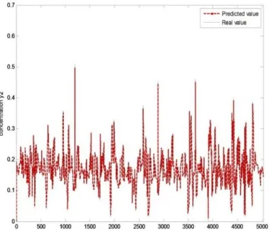
Figure 5. y2 content prediction in SRU (Validation data)
Comparison between real and predicted results of C4 concentration in Figures 7 and 8 demonstrate well accordance, even with missing data existence in observed data. The missing data are generated by an interpolation that is based on the estimated model and the data on both sides of the gap.
Also, Figures 9 and 10 show the most of the predicted values are consistent with the 45° line, that imply the good performance of the soft sensors model.
Figure 6. DARX model parameters results versus samples for SRU
Figure 7. Comparison between real and predicted results of y1 concentration(Validation data), (a) without missing
values in dataset, (b) with random missing values
Figure 8. Comparison between real and predicted results of y2 concentration(Validation data), (a) without missing
Figure 10. Predicted valueagainst real value of y2
concentration
As a consequence, this work indicates that the DARX model is associated with the highest correlation coefficient and the lowest RMSE and MAE compared to MLP [41, 43], the different type of PLS [42] and other presented methods in Table 4.
4.CONCLUSION
A new model for online soft sensing with TVP approach, was performed. The quality prediction was implemented by a data-driven model that is a combination of nonlinear correlation analysis, DARX model and also criterion-based elimination method. This model can successfully supported the nonlinear and time-variant systems. The result showed very good performance between predicted and real value, in industrial SRU, even with random missing value in datasets. A part of industrial SRU data was implemented for model validation. The results of parameters prediction and transfer function models estimation with low complexity by this technique was indicated the maximum prediction accuracy, minimum error and more appropriate performance indexes compared to models that implemented by other researchers about SRU (Table 4). It should be mentioned that although the employed methods, nonlinear correlation analysis, and criterion-based elimination, are not new.
TABLE 4. The reported performance index of SRU soft sensor
Type of model Number of variables R RMSE MAE AIC YIC Ref.
MLP: H2S
SO2
RBF1: H
2S
SO2
NF2: H
2S
SO2
Nonlinear LSQ3: H
2S
SO2
Not reported
(0.851 0.919) (0.939
0.941) (0.843 0.852)
(0.858 0.897)
(0.0282 0.0173) (0.0141
0.0141) (0.0300 0.0244)
(0.0264 0.0200)
Not reported Not reported Not reported [41]
JITPLS4: H 2S
SO2
RPLS5: H
2S
SO2
OLPLS6: H 2S
SO2
-- Not reported
(0.0210 0.0238) (0.0196
0.0209) (0.0162 0.0142)
(0.1647 0.1411) (0.1783
0.1964) (0.2138 0.1174)
-- -- [42]
MLP: (H2S) 16 0.9236 Not reported -- -- -- [43]
MLP: (H2S) 11 0.9438 -- -- -- -- [44]
TDGPR7: (H
2S) 5 Not reported 0.0168 -- -- -- [45]
DARX: H2S
SO2
2 2
0.9507 0.9648
0.0158 0.0138
0.0024 0.0018
-8.1474 -8.5047
-7.3544
-8.2521 This work
1.Radial Basis Function, 2.Neuro-Fuzzy, 3.Least Square, 4.just-in-time PLS, 5.Recursive PLS, 6.Online Local PLS, 7.Time Difference Gaussian Process Regression
Figure 9. Predicted valueagainst real value of y1
However, the integration of these techniques by DARX model as an industrial solution which is easy to implement, allow engineers to design the high-performance soft sensor for online quality estimation. Due to satisfactory prediction performance and rapid converge of the quasi-linear model in industrial control processes is very effective.
5. REFERENCES
1. Fortuna, L., Graziani, S. and Xibilia, M.G., "Soft sensors for monitoring and control of industrial processe, NewYork, Springer, (2007).
2. Ramli, N.M., Hussain, M.A., Jan, B.M. and Abdullah, B., "Composition prediction of a debutanizer column using equation based artificial neural network model", Neurocomputing, Vol. 131, No., (2014), 59-76.
3. Fortuna, L., Graziania, S. and Xibilia, M.G., "Soft sensors for product qualitymonitoring in debutanizer distillation columns",
Control Engineering Practice, Vol. 13, (2005), 499-508. 4. Kadlec, P., Gabrys, B. and Strandtb, S., "Data-driven soft sensors
in the process industry", Computers and Chemical Engineering, Vol. 33, (2009), 795–814.
5. Pani, A.K., Amin, K.G. and Mohanta, H.K., "Soft sensing of product quality in the debutanizer column with principal component analysis and feed-forward artificial neural network",
Alexandria Engineering Journal, Vol. 55, (2016), 1667- 1674. 6. Kano, M., Showchaiya, N., Hasebe, S. and Hashimoto, I., "Hashimoto, inferential control of distillation compositions: Selection of model and control configuration", Control Engineering Practice, Vol. 11, No. 8, (2003), 927- 933.
7. Kim, S., Okajimaa, R., Kanob, M. and Hasebe, S., "Development of soft sensor using locally weighted pls with adaptive similarity measure", Chemometrics and Intelligent Laboratory Systems, Vol. 124, (2013), 43- 49.
8. Komulainena, T., Souranderb, M. and Jämsä-Jounela, S.-L., "An online application of dynamic pls to a de-aromatization process",
Computers & Chemical Engineering, Vol. 28, No. 12, (2004). 9. Shao, W., Tian, X., Wang, P., Deng, X. and Chen, S., "Online soft
sensor design using local partial least squares models with adaptive process state partition", Chemometrics and Intelligent Laboratory Systems, Vol. 144, (2015), 108- 121.
10. Ge, Z. and Song, Z., "Semi supervised bayesian method for soft sensor modeling with unlabeled data samples", AIChE Journal, Vol. 57, No. 8, (2011), 2109–2119
11. Wang, Y.-J., Jia, M.-X. and Mao, Z.-Z., "A fast monitoring method for multiple operating batch processes with incomplete modeling data types", Journal of Industrial and Engineering Chemistry, Vol. 21, (2015), 328-337.
12. Zhang, X., Yan, W., Zhao, X. and Shao, H., "Nonlinear real-time process monitoring and fault diagnosis based on principal component analysis and kernel fisher discriminant analysis",
Chemical Engineering & Technology, Vol. 30, No. 9, (2007), 1203–1211.
13. Ma, M.-D., Kob, J.-W., Wang, S.-J., Wud, M.-F., Jangd, S.-S., Shiehe, S.-S. and Wong, D.S.-H., "Development of adaptive soft sensor based on statistical identification of key variables",
Control Engineering Practice, Vol. 17, No. 9, (2009), 1026- 1034.
14. Chew, C.M., Aroua, M.K. and Hussain, M.A., "A practical hybrid modelling approach for the prediction of potential fouling parameters in ultrafiltration membrane water treatment plant",
Journal of Industrial and Engineering Chemistry, Vol. 45, (2017), 145-155.
15. Naeini, M.K. and Bayati, N., "Pattern recognition in control chart using neural network based on a new statistical feature",
International Journal of Engineering, Vol. 30, No. 9, (2017), 1372-1380.
16. Park, S. and Ha, C., "A nonlinear soft sensor based on multivariate smoothing procedure for quality estimation in distillation columns", Computers & Chemical Engineering, Vol. 24, No. 2-7, (2000), 871- 877.
17. Kadlec, P. and Gabrys, B., "Adaptive local learning soft sensor for inferential control support", in Computational Intelligence for Modelling Control & Automation, Vienna, Austria IEEE., (2008 of Conference).
18. Radhakrishnan, V.R. and Mohamed, A.R., "Neural networks for the identification and control of blast furnace hot metal quality",
Journal of Process Control, Vol. 10, No. 6, (2000), 509- 524.
19. Liu, Y. and Chen, J., "Integrated soft sensor using just-in-time support vector regression and probabilistic analysis for quality prediction of multi-grade processes", Journal of Process Control, Vol. 23, No. 6, (2013), 793-804.
20. Jin, H., Chen, X., Yang, J. and Wu, L., "Adaptive soft sensor modeling framework based on just-in-time learning and kernel partial least squares regression for non- linear multiphase batch processes", Computers & Chemical Engineering, Vol. 71, (2014), 77-93.
21. Fujiwara, K., Kano, M., Hasebe, S. and Takinami, A., "Soft-sensor development using correlation-based just-in-time modeling", AIChE Journal, Vol. 55, No. 7, (2009), 1754-1765. 22. Kadlec, P. and Gabrys, B., "Adaptive online prediction soft sensing without historical data", in Neural Networks (IJCNN), The 2010 International Joint Conference, Barcelona, Spain IEEE., (2010 of Conference), 1-8.
23. Ge, Z. and Song, Z., "A comparative study of just-in-time-learning based methods for online soft sensor modeling",
Chemometrics and Intelligent Laboratory Systems, Vol. 104, No. 2, (2010) 306-317.
24. Bosca, S. and Fissore, D., "Design and validation of an innovative soft-sensor for pharmaceuticals freeze-drying monitoring",
Chemical Engineering Science, Vol. 66, No. 21, (2011), 5127- 5136.
25. Khatibisepehr, S., Huang, B. and Khare, S., "Design of inferential sensors in the process industry: A review of bayesian methods",
Journal of Process Control, Vol. 23, No. 10, (2013), 1575- 1596. 26. McIntyre, N., Young, P., Orellana, B., Marshall, M., Reynolds, B. and Wheater, H., "Identification of nonlinearity in rainfall-flow response using data-based mechanistic modeling", Water Resources Research, Vol. 47, No., (2011). doi: 10.1029/2010WR009851
27. Abbasi, M., Soleymani, A.R. and Parssa, J.B., "Operationsimulation of a recycled electrochemical ozone generator using artificial neural network", Chemical Engineering Research and Design, Vol. 92, No. 11, (2014), 2618–2625. 28. Hosen, M.A., Khosravi, A., Nahavandi, S. and Creighton, D.,
"Prediction interval-based neural network modeling of polystyrene polymerization reactor—a new perspective of data-based modeling", Chemical Engineering Research and Design, Vol. 92, No. 11, (2014), 2041–2051.
Computers & Chemical Engineering, Vol. 30, No. 3, (2006), 508-520.
30. Bidar, B., Sadeghi, J., Shahraki, F. and Khalilipour, M.M., "Data-driven soft sensor approach for online quality prediction using state dependent parameter models", Chemometrics and Intelligent Laboratory Systems, Vol. 162, (2017), 130–141. 31. Taylor, C.J., Pedregal, D.J., Young, P. and Tych, W.,
"Environmental time series analysis and forecasting with the captain toolbox", Environmental Modelling & Software, Vol. 22, (2007), 797-814.
32. Young, P.C., "Recursive estimation and time-series analysis", Seconded ed, New York, Springer, (2011).
33. Young, P.C., MCKENNA, P. and BRUUN, J., "Identification of non-linear stochastic systems by state dependent parameter estimation", International Journal of Control, Vol. 74, (2001), 1837-1857.
34. Pedregal, D.J., Taylor, C.J. and Young, P.C., "System identification, time series analysis and forecasting: The captain toolbox handbook, Faculty of Science and Technology, Lancaster Environment Centrer, Lancaster University, United Kingdom, (2007).
35. Sadeghi, J., "Modelling and control of non-linear systems using state-dependent parameter (SDP) models and proportional-integral-plus (pip)control method", Lancaster University, Centre for Research on Environmental System and Statistics, United Kingdom, PhD, (2006),
36. Young, P.C., Data-based mechanistic modeling: Natural philosophy revisited?, in System identification, environmental modelling, and control system design. 2011, Springer. 321-340.
37. Young, P.C., kenna, P.M. and Bruun, J., "Identification of nonlinear stochastic systems by state dependent parameter estimation", International Journal of Control, Vol. 74, No. 18, (2001), 1837-1857.
38. Snipes, M. and Taylor, D.C., "Model selection and akaike information criteria: An example from wine ratings and prices",
Wine Economics and Policy, Vol. 3, No. 1, (2014), 3-9. 39. Dziak, J., Li, R. and Collins, L., Critical review and comparison
of variable selection procedures for linear regression (technical report). 2005, Methodology Center, Penn State University. 40. Lees, M.J., "Data-based mechanistic modeling and forecasting of
hydrological systems", Journal of Hydroinformatics, Vol. 2, No. 1, (2000), 15-34.
41. Fortuna, L., Rizzo, A., Sinatra, M. and Xibilia, M.G., "Soft analyzers for a sulfur recovery unit", Control Engineering Practice, Vol. 11, No. 12, (2003), 1491-1500.
42. Shao, W., Tian, X. and Wang, P., "Local partial least squares based online soft sensing method for multi-output processes with adaptive process states division", Chinese Journal of Chemical Engineering, Vol. 22, No. 7, (2014), 828- 836.
43. Graziani, S., Napoli, G. and Xibilia, M.G., "Soft sensor design for a sulfur recovery unit using a clustering based approach", in Measurement Technology Conference, Victoria, BC, Canada IEEE, (2008 of Conference).
Online Monitoring for Industrial Processes Quality Control Using Time Varying
Parameter Model
R. Parvizi Moghadam, F. Shahraki*, J .Sadeghi
Center for Process Integration and Control (CPIC), Department of Chemical Engineering, University of Sistan and Baluchestan, Zahedan, Iran
P A P E R I N F O
Paper history:
Received 22 November 2017
Received in revised form 31 December 2017 Accepted 04 Januray 2018
Keywords: Soft Sensor
Time Varying Parameter SRU
Quality Estimation Identification Data- based Modeling
هديكچ
هداد مرن رگسح کی شیپ یارب دیدج روحم
هدش یحارط یتعنص یاهدحاو رد لوصحم تیفیک لرتنک درکلمع دوبهب و نیلانآ ینیب
یرتماراپ لدم یبیکرت درکیور .تسا (نامز اب ریغتم
TVP
(نویسرگردوخ یجراخ ریغتم یکیمانید متیروگلا ،)
DARX
زیلانآ ،)
هلیسو هب مرن رگسح درکلمع رابتعا .تسا هدش یفرعم قیقحت نیا رد درکلمع یبایزرا رایعم اب یفذح شور و یطخریغ یگتسبمه هداد زا یشخب تمواقم رب جیاتن .دش یبایزرا درگوگ تفایزاب دحاو یتعنص یاه
بسانم یدرکلمع صخاش و رتشیب رد رگسح نیا رت
شور زا لصاح جیاتن اب هسیاقم تللاد ،درگوگ تفایزاب دحاو مرن رگسح یحارط یارب تاقیقحت ریاس رد هدش هتفرگ راک هب یاه
هطساو هب .تشاد شیپ تقد ی
هفرص و لصاح لدم یگدیچیپ مدع ،لااب ینیب یم کینکت نیا ،نامز رد ییوج
تنک رد دناوت یاهدنیارف لر
.دریگ رارق هجوت دروم رایسب یتعنص