Comparing Different Models of Evolutionary Three-Objective
Optimization Using Fuzzy Logic in Tehran Stock Exchange
Mohammad Javad Salimi 1
Mir Feiz Fallah2
Hadi Khajezadeh Dezfuli3
Abstract
Optimal Portfolio Selection is one of the most important issues in the field of financial research. In the present study, we try to compare four various different models, which optimize three-objective portfolios using “Postmodern Portfolio Optimization Methods”, and then to solve them. These modeling approaches take into account both multidimensional nature of the portfolio selection problem and requirements imposed by investors. Concretely different models optimize the expected return, the down side risk, skewness and kurtosis given portfolio, taking into account budget, bounds and cardinality constrains. The quantification of uncertainty of the future returns on a given portfolio is approximated by means of LR-fuzzy numbers, while the moments of its returns are evaluated using possibility theory. In order to analyze the efficient portfolio, which optimize three criteria simultaneously, we build a new NSGAII algorithm, and then find the best portfolio with most Sortio ratio from the gained Pareto frontier. Thus, in this paper we choose 153 different shares from different industries and find their daily return for ten years from April of 2006 till March of 2017 and then we calculate their monthly return, downside risk, skewness, kurtosis and all of their fuzzy moments. After designing the four models and specific algorithm, we solve all of the four
1. Ph.D. in Accounting, Assistant Professor, Allameh Tabatabaei University [email protected] 2. Ph.D. in Finance, Associate Professor, Islamic Azad University, Central Tehran Branch
Iranian Journal of Finance
84
models for ten times and after collection of a table of the answers, compare all of them with Treyner ratio. At last, we find that using fuzzy and possibistic theory make higher return and better utilized portfolios.
Key words: Modern Portfolio Theory, Post Modern Portfolio Theory, Financial Modeling, Optimize Portfolio Selection, Evolutionary Multi-Objective Algorithm, Fuzzy Logic
1. Introduction
Optimal Portfolio Selection is one of the most important issues in the field of financial research. This means what combination of assets the investor should choose to maximize the utilization with relevant limitation. Markowitz considered returns as a random variable and solved this problem with maximization of return and minimization of variance as risk criteria. However, return on securities in the real world is usually vague and inaccurate. In today's world of investment, one of the challenges of investment in return on assets is uncertainty of future events and their consequences.
Solving the problem of selecting portfolios requires two key components: a) A suitable method for quantitatively measuring the uncertainty of future returns of the desired portfolio; and b) The optimization procedure and method that can provide Pareto optimal portfolios that meet the investors’ requirements (D.Dubois, Prade, 1980)
In the recent years, there has been a growing interest of including information about trading and investors’ requirements into the portfolio selection problem, since not all the relevant information for portfolio selection can be obtained just by optimizing returns and risk simultaneously. Thus, some practical constraints have been added to portfolio selection problem in order to make it more realistic, such as upper and lower bound constrains, allowing asset combinations which respect the investors’ wishes, or cardinality constrains limiting the number of assets participating in the portfolios. With the introduction of such constraints, the portfolio optimization problem becomes a constrained multi-objective problem that is NP-hard, and traditional optimization methods cannot be used to find efficient portfolios (Reben Saborido, Ruiz, Bermudez, Vercher, 2016).
Comparing Different Models of Evolutionary Three 85
simultaneously optimization of three-objective modelling, by using mean, downside risk, skewness and kurtosis. After that, we design a new method of NSGAII algorithm to solve models and finally, we conclude that using fuzzy logic has a positive effect on portfolio optimization process and using skewness in three-objective modeling can make much better portfolios than using kurtosis.
1. Formulation and Background Concepts
Multi-objective optimization problems are mathematical programming problems with a vector-valued objective function, which is usually denoted by f(x) = (f1(x), ... fn(x)) for a decision vector x=(x1,...,xN), where fj(x) is a real-valued function defined over the feasible set S⊆RN, for every j=1,..,n. Consequently, the decision space belongs to RN, while the criterion space belongs to Rn, and the multi-objective optimization problem can be stated as follows:
Optimize: }f1(x), …,fn(x){ (1) s.t. x ∈ S.
In the criterion space, some objective functions must be maximized (j∈J1) while others must be minimized (j∈J2), where J1 and J2 verify that
J1 J2 {1 , ...., n} and J1 J2 .
We say that x∈ S is Pareto optimal or efficient solution if there does not exist another x’∈ S, such that f (x )J f (x)j for every j∈J1 and f (x )J f (x)j for
every j∈J2 . with at least one strict inequality. The set of all Pareto optimal solutions x ∈ S.(in the decision space) is called the Pareto optimal set, denoted by E, and the set of all of their corresponding objective vectors f(x) (in the criterion space) is called the Pareto optimal front, denoted by f(E). Additionally, given two objective vectors z, z’∈ Rn , we say that z’ dominated z if and only if z’j zj for every j≥ ∈J1 and zj z’j for every j≥ ∈J2 with at least one strict inequality. If z and z’ do not dominate each other, they are said to be non-dominated (Reben Saborido,Ruiz, Bermudez, Vercher, 2016).
Iranian Journal of Finance
86
respectively. The ideal point z*= (z1*,… , zn*)T ∈ Rn is obtained by optimizing each objective function individually over the feasible set, that is z*j =maxx s = f(x) = maxx s f(x) for every j∈J1 and z*j = maxx s = f(x) = minx s
for all j∈J2 . The nadir point znad= (z1nad …, znnad)T ∈ Rn is defined as znadj = min f (x)j x s for all j∈J1 and znadj = max f (x)j x s for all j∈J2. In
practice, the nadir point is difficult to calculate and the general practice is to estimate it with different approaches {38, 39}. Sometimes, a vector that dominates every Pareto optimal solution is required, which means that it is strictly better than the ideal point. This vector is denoted by z**= (z1**,… , zn**)T and it is called a utopian point. In practice z** can be defined by
** *
j j j
Z Z for all j∈J1 and Z**j Z*j j j∈J2, where j 0 is a small real
number for every j = 1, …,n (Reben Saborido, Ruiz, Bermudez, Vercher, 2016).
The use of evolutionary multi-objective optimization (EMO) algorithm for solving multi-objective optimization problems has become very popular in the last two decades and, currently it is one of the most active research fields [3.4]. In the EMO field, solving a multi-objective optimization problem is understood as finding a set of non-dominated solution as close as possible to Pareto optimal front (diversity). EMO algorithms are population-based approaches which start with randomly created population of individuals. Afterwards, the algorithm enters in an iterative process that creates a new population at each generation, by the use of operators which simulates the process of natural evolution: selection, crossover, mutation and/or elitism preservation. One of the main advantages of EMO algorithms is that they are very versatile, as they can deal with multi-objective optimization problems having variables and objective functions of different nature (X. Zou, Chen, Liu, Kang, 2008).
Comparing Different Models of Evolutionary Three 87
solution constitute the so-called first non-dominated front. These individuals are temporarily removed and, subsequently, the second non-dominated front is formed by next individuals, who are not dominated by any other solution in the population. This process continues until every individual has been included into a single front. Afterwards, the population to be passed to the next generation is formed by the solutions in the lower level of non-dominated fronts.
2. Previous related works
While classical portfolio optimization problems can be efficiently solved by applying classical optimization techniques, this is not the case if additional conditions, such as diversification and cardinality constraints, are introduced. Mainly, the most significant difficulty is the generation of feasibility portfolios satisfying the requirements imposed by investors. Additionally, the solution process required for finding the set of efficient portfolios is not trivial. Note that the management of non-dominated solution is computationally simple in the bi-objective case, but it is much complicated in presence of multi-objective (three of more). In this regard, the usefulness of evolutionary multi-objective optimization for solving the constrained multi-objective portfolio selection problem is doubtless because of its ability to handle multiple criteria and constraints at the same time (K. Liagkouras, Metaxiotis, 2015). The reason for such a success is that they work with the problem as a black box, only considering inputs and outputs, without requiring additional information like derivation or continuity of properties of objective functions (Khajezadeh Dezfuli, Mehdi, 2016).
For example, Chang et al. (T.J.Chang, Meade, Beasley, Sharaiha, 2000) applied these types of algorithms to the mean-variance (MV) model. They showed that limiting the number of assets in portfolio (i.e including cardinality constraints) and considering lower and upper bounds for budget invested in such assets modify the shape of Pareto optimal front. They demonstrated that in the presence of constraints, the Pareto optimal front of MV model is more difficult to approximate, because it may become discontinuous.
Iranian Journal of Finance
88
procedure was suggested, while Moral-Escudero et al. (R.Moral-Escudero, Ruiz-Torrubiano, Suarez, 2006) used a hybrid strategy that made use of genetic algorithms and quadratic programming for selecting the optimal subset of assets. In (R.Moral-Escudero, R.Ruiz-Torrubiano, A.Suarez, 2007), an EMO algorithm was combined with fuzzy logic in order to facilitate the trade-off between the two objectives. They also analyzed the performance of several EMO algorithms for solving the constrained MV portfolio optimization problem. For solving the cardinality constrained MV model, Chiam et al. (S.C.Chiam, Tan, Mamum, 2008) proposed an order-based representation with suitable variation operator and some techniques for handling constraints. More recently, Anagnostopoulos and Mamanis (K.P. Anagnostopoulos, G.Mamanis, 2008), applied three EMO algorithms in order to explore the Pareto optimal Front if cardinality was included into the MV model as an additional objective to be minimized. Also, Anagnostopoulos and Mamais (S.C.Chiam, Tan, Mamum, 2008) presented a study in which five EMO approaches were applied to the cardinality constrained MV model for solving instances of data sets with large number of assets, showing a clear superiority of the evolutionary algorithms SPEA2(Zitzler, M.Laumanns, L.Thiele, 2001) and NSGAII (K.Deb, Pratap, Agarwal, Meyarivan, 2002). Lately, Liagkouras and Metaxiotis (K.Liagkouras, Metaxiotis, 2014) have proposed a mutation operation for solving the cardinality constrained MV model, which was compared with the classical polynomial mutation operator also in NSGAII and SPEA2.
Other authors solve portfolio selection models with the alternative measure of risk and/or additional constraints by means of EMO algorithms. For example, Chang et al. (T.J.Chang, Yang, Chang, 2009) applied a genetic algorithm for solving bi-objective optimization portfolio selection problem with different risk measures (variance, semi-variance, absolute deviation), including skewness as a constraint. These authors reported the fact that investors should not consider portfolio sizes above one third of the total number of assets, because they are dominated by other portfolios with less positive components.
Comparing Different Models of Evolutionary Three 89
uncertainty of future returns on assets, using credibility or possibility distribution. For example Bhattacharyya et al. (R.Bhattacharyya, Kar, Majumder, 2011) considered a fuzzy mean-variance-skewness model with cardinality and trading constraints, which is solved by applying both fuzzy simulation and an elitist optimization genetic algorithm. Bernidez et al. (D.Bermudez, Segura, Vercher, 2012) implemented a bi-objective optimization genetic algorithm for solving a fuzzy mean-downside risk portfolio selection problem with cardinality constraints and diversification conditions, in which the approximation of the uncertain returns was done through trapezoidal fuzzy numbers. In (P.Gupta, Inuiguchi, Mehlawat, Mittal, 2013), a multi-criteria credibilistic portfolio selection model was proposed, which maximized (short and long–term) return and liquidity and considered the portfolio risk as a credibility-based fuzzy chance constraint. The fuzzy estimates were obtained assuming both trapezoidal possibility distributions and general functional forms. This model, which also included budget, bound and cardinality constraints was solved by applying a hybrid algorithm that integrated fuzzy simulation with a real-coded genetic algorithm.
2.1. Fuzzy background
In the portfolio optimization problem, the modeling of uncertain returns on assets is made using different approaches. Some authors assume that these returns are random variables, while others consider fuzzy logic to integrate the uncertainty of the datum, imperfect knowledge of market behavior, imprecise investors' aspirations levels and experts opinion and so on. However, expected return on asset modeling either as random variable or fuzzy quantities are consider as known parameters of optimization problem, which have been usually estimated throughout historical data set (Reben Saborido, Ruiz, Bermudez, Vercher, 2016).
Iranian Journal of Finance
90
denoted by rt(x)Tt 1 , are used as the historical data set, and the possibility of
distribution of return on x allows us to evaluate their corresponding interval-mean valued expectations. Let us briefly review some definitions and results required about fuzzy set theory (D.Dubois, Prade, 1978 , 1980, M.Inuiguchi, T.Tanino,2002).
A fuzzy number Q is said to be an LR-type fuzzy number if its membership function has the following form:
Where A and B satisfy A≤B, and represent the lower and upper bounds of the core of Q representatively, i.e., {y| } =]A, B [that SA و SB are
the left and the right spread of Q and L, R: ]0, + ∞)→]0, 1 [ are reference functions which are non-increasing and upper semi-continuous with . A fuzzy number Q is said to be bounded LR-type fuzzy number if the reference functions are such that the support of Q is bounded, i.e., if there exist two real numbers a and b, with a>b, such that
{y: ]a, b[.
For a portfolio x, let us consider the reference function
and , where and are their positive shape parameters,
respectively, for every t =1,…,T. Thus, we have a power LR-fuzzy number Q induced a possibility distribution that matches with its membership function (L.A.Zadeh, 1978), we consider power LR-fuzzy number to
Comparing Different Models of Evolutionary Three 91
mentioned that other weighted mean-interval definitions could be used analogously (R.Fullér, Majlender, 2003).
First possibilistic moment:Possibilistic mean value
=
Second possibilistic moment:
Possibilistic downside risk
Third possibilistic moment:
Possibilistic Skewness
Forth possibilistic moment:
3. Modeling
In this section, we describe several models that we have used to determine the best portfolio selection, and after that, we will solve the models, compare the results, and rank them.
Let us consider a capital market with N financial assets offering uncertain rates of returns. As the investor desires to know which optimal allocation of their wealth exists among the N assets, the maximization of of investment return at the end of the period is looked for. Let us consider a portfolio x=(x1, x2, …, xN)T in which the total wealth is allocated, where xi is a fraction of the total investment devoted to the asset i, for every i=1,…,N. The portfolio must verify that
N
i i 1
x
1
And the non-negative condition of every proportion, xi 0 for every i=1, …, N when short selling is excluded. In the models, the expected return on asset i and its possibilistic moments are not considered as known parameters. The possibility distribution of a given portfolio is directly approximated instead of using aggregation of the possibility distribution of the individual assets, as mentioned before. According to this, the return of portfolio x is modeled by the power of LR-fuzzy number, denoted by Px(p , p , c, d)1 u L R whose cord and
Iranian Journal of Finance
94
Additionally, we imposed limits on the budget to be invested in each asset i by using lower and upper bounds, denoted by liand ui, respectively, for every i=1, …, N. Besides, in order to control the number of assets in the portfolio, an additional constraint is incorporated to assure that the number of non-negative components in each portfolio is within an interval [kl,ku], for given values kl and ku.
Based on aforementioned assumptions, the cardinality constrained, we design four different models as follow:
(1)fuzzy mean, fuzzy downside risk, fuzzy skewness
(
1
)
(
2
)
(
3
)
St
(
4
)
(
5
) (
6
)
That is possibilistic expected return, possibilistic semi-deviation
below mean is , is the possibilistic skewness.
(2)fuzzy mean, fuzzy downside risk, fuzzy kurtosis
(
7
)
(
8
)
(
9
)
Comparing Different Models of Evolutionary Three 95
(
10
)
(
11
) (
12
)
That is possibilistic expected return, is the possibilistic
semi-deviation below mean, and is the possibilistic kurtosis.
(3) mean, downside risk, skewness
(
13
)
(
14
)
(
15
)
St
(
16
)
(
17
) (
18
)
That is the expected return, is the semi-deviation below mean, and
is the possibilistic skewness.
(4) mean, downside risk, kurtosis
(
19
)
(
20
)
(
21
)
Iranian Journal of Finance 96 ( 22 ) ( 23 ) ( 24 )
4. Portfolio selection problem
Clearly, the creation of a suitable structure for the chromosome in a multi-objective genetic algorithm can have a significant effect on the quality and efficiency of this algorithm. In fact, a suitable structure for the chromosome can lead to a full space search, and the result of the algorithm will be a better answer. What makes it difficult to use this algorithm in this problem is the two-step problem solving. This means that we must first agree on the number of shares available per portfolio, and then determine the amount of investment in the shares in that portfolio. The chromosome designed in this paper solves the problem and solves the problem by creating the same structure for all chromosomes (Mehdi Khajezadeh Dezfuli, 2016). The following figure shows an example of a chromosome designed:
0.21 0.84 0.65 ... 0.91 0.03 0.19 0.38
1 2 3 ... 152 153 154 155
0.51 0.83 156 157 0.13 0.71 158 159 0.90 0.09 160 161 0.35 0.64 162 163 0.59 164 0.53 0.81 165 166
The designed structure consists of three main parts. In the first part of the chromosome, all existing companies in the problem (153 shares) are considered. The second part consists of a cell that is shown in green and is used to determine the number of shares in each portfolio, and the third part consists of orange cells that are used to select portfolios. All these cells are assigned a random number between 0 and 1, and then by the defined function, these values are converted to the main values of the problem. Initially, using the
To select shares from existing shares
To determine the number of shares of each portfolio
Comparing Different Models of Evolutionary Three 97
number contained in cell 154 and using the spacing taken between 0 and 1, and the location in each range, the number of shares in the portfolio is determined. Then, in the same way and with the function that is defined, the numbers in the orange cells determine the shares to be selected from among the existing 153 shares. At this point, a specific portfolio has been created, with numbers between 0 and 1; now, to determine the amount of investment per share, each of these numbers is divided by the total number of available portfolios in order to determine the percentage of investment per share. The total percentage values will be equal to one. Finally, using the values of the variables and the problem data, the objective functions of the model are calculated. The obvious characteristics of the chromosome can be pointed out that all the problem constraints in the created structure are observed, and that no irrelevant answer will be generated. So you can be sure that the final answer will be questionable.
4.1. Multi-objective genetic algorithm operators
Two operators perform the search process in the multi-objective genetic algorithm: mutation and crossover. The reproduction operator is used to extract better answers; while mutation operator is used to explore the broader response space, the crossover is used to extract better answers (Mehdi Khajezadeh Dezfuli, 2016).
4.1.1. Crossover operator
Iranian Journal of Finance
98
0.35 0.19 0.91 ... 0.83 0.52 0.06
0.67 0.51 0.33 ... 0.16 0.88 0.23
0.67 0.51 0.33 ... 0.83 0.52 0.06
0.35 0.19 0.91 ... 0.16 0.88 0.23 Parent 1
Parent 2
Offspring 1
Offspring 2
Crossover point
4.1.2. Mutation operator
There are several types of mutant operators that are used in the multi-objective genetic algorithm. Items such as Swap, Insertion and Inversion are used. All of these methods are used in this article. Firstly, a chromosome is selected using the roulette wheel method. The numbers 1 to 3 are assigned to mutant operators, respectively, and then a random number is generated between the interval (Enriqueta Vercher, Bermudez, 2015), which determines which operator to use. An example of a succession operator is shown in the following figure:
0.35 0.19 0.91 ... 0.83 0.52 0.06 Swap 0.35 0.83 0.91 ... 0.19 0.52 0.06
5. Research hypotheses
There is no significant difference between the performance of three-objective evolutionary models, mean-downside skewness, mean-downside risk-kurtosis, fuzzy mean-fuzzy downside risk-fuzzy skewness and fuzzy mean- fuzzy downside risk- fuzzy kurtosis.
Comparing Different Models of Evolutionary Three 99
The population of the research is the industries listed in Tehran Stock Exchange with two criteria: A) Market concentration and turnover B) Number of companies accepted in the industry. Thus, the 35 industries listed on Tehran Stock Exchange, out with the exception of industries such as banks and credit institutions, insurance and pension funds, investment companies, Holdings and other financial intermediation (which are characterized by unusual capital structure and different reporting practices and can lead to data deviations), industries that are more exposed to market players and include at least 10 active and qualified companies were selected as the statistical sample of the survey.
7. Research method
This research is practical in terms of the purpose. In terms of the method of implementation, it is a descriptive research and it is a correlation analysis. This research can be considered as a post- traumatic research. The research steps were as follow:
1. In the first step, the data were collected.
2. Daily returns of each company were extracted from the TSETMC website and “Rahavard Novin” software, and the monthly return, downside risk, skewness and kurtosis for each company were calculated.
3. Quartiles of returns were determined and fuzzy return, fuzzy downside risk, fuzzy skewness, and fuzzy kurtosis were calculated and then, the numbers were converted to crisp numbers.
4. Interest of the Investor involved for investment in each company (up to 60% of the total initial arrival) and the number of portfolio members (between four and twelve shares).
Iranian Journal of Finance
100
15%. After that, each of the models was executed ten times and Pareto frontier was obtained.
6. The best portfolios were chosen from the Pareto frontier using the Sortino ratio.
7. To compare the extracted portfolios, the trainer's ratio was used, using the actual data of 2016-17, the summary of which is given in Table 1. 8. The variance analysis was used to compare the performance of the
models.
8. Numeral results
In this section, all different scenarios examined will be compared in three-objective programming models and the results will be presented.
1. Results from three-objective planning models
Fuzzy Mean- Fuzzy downside
risk- Fuzzy kurtosis
Fuzzy Mean - Fuzzy downside
risk - Fuzzy skewness Mean-downside risk- kurtosis Mean-downside risk- skewness
22/73 33/41 5/54 19/65
Treyner ratio Fuzzy Mean- Fuzzy downside
risk- Fuzzy kurtosis
Treyner retio of Fuzzy Mean - Fuzzy downside
risk - Fuzzy skewness Treyner ratio of Mean-downside risk- kurtosis
Treyner ratio of Mean-downside risk- skewness
16/58 -0/23 1/39 -6/57
Then the results of two different models of Mean-Downside risk-Skewness and Mean-Downside risk-Kurtosis will be compared:
2. T student test: Mean-Downside risk-Skewness and Mean-Downside risk-Kurtosis
ITEM COMPARATIVE ITEMS STATISTICAL
VALUE
CRITICAL
VALUE Pvalue
APPROVED HYPOTHISES
1 Return of the models 3.81 2.262 0.0042 H1
Comparing Different Models of Evolutionary Three 101
As indicated in Table 2, the average returns from ten times
implementation
of the planning model of Mean-Downside
risk-Skewness
is much better than implementation of the planning
model of Mean-Downside risk-Kurtosis, and create more return.
The rejection of the assumption of H0 also shows that the results
are not coincidental and the t test also confirms these results.
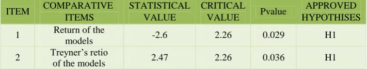
3. T student test: Fuzzy Mean-Fuzzy Downside risk- Fuzzy Skewness and Fuzzy Mean- Fuzzy Downside risk - Fuzzy Kurtosis
ITEM COMPARATIVE ITEMS
STATISTICAL VALUE
CRITICAL
VALUE Pvalue
APPROVED HYPOTHISES
1 Return of the
models -2.6 2.26 0.029 H1
2 Treyner’s retio
of the models 2.47 2.26 0.036 H1
Table 3 shows that the H0 assumption is rejected in relation to the comparison of the two above models, which indicates that the difference between the obtained numbers is not accidental and reliable. Therefore, it can be concluded that the efficiency of the planning model is Fuzzy Mean-Fuzzy Downside risk-fuzzy Kurtosis is better than the Mean- Downside risk- Kurtosis.
4. T student test: Fuzzy Mean-Fuzzy Downside risk- Fuzzy Skewness and Mean- Downside risk - Skewness
ITEM COMPARATIVE ITEMS
STATISTICAL VALUE
CRITICAL
VALUE Pvalue
APPROVED HYPOTHISES
1 Return of the
models -2.26 2.262 0.0497 H1
2 Treyner’s retio
of the models 6.37 2.26 0.00013 H1
Iranian Journal of Finance
102
Fuzzy Downside risk - Fuzzy Skewness is better than the programming model Mean – Downside risk – Skewness.
5. T student test: Fuzzy Mean-Fuzzy Downside risk- Fuzzy Kurtosis and Mean- Downside risk - Kurtosis
ITEM COMPARATIVE ITEMS
STATISTICAL VALUE
CRITICAL
VALUE Pvalue
APPROVED HYPOTHISES
1 Return of the
models -3.45 2.26 0.007 H1
2 Treyner’s retio
of the models 2,57 2.26 0,045935512 H1
As shown in Table 5, the average returns from ten times implementation of the planning model of fuzzy Mean-fuzzy downside risk-fuzzy Kurtosis, is better than Mean-Downside risk-Kurtosis.
9. Conclusion
Comparing Different Models of Evolutionary Three 103
References
1. D.Dubois, H.Prade, (1980), Fuzzy Sets and Systems Theory and Applications, 2. Demic Aca-press, NewYork.
3. Reben Saborido, Ana B.Ruiz, Jose D.Bermudez, Enriqueta Vercher, Applied soft computing 39 (2016) 48-63
4. C.A.C. Coello, G.B. Lamont, D.A.V. Veldhuizen, (2001), Evolutionary Algorithms for Solving Multi-Objective Problems, 2nd ed. Springer,New York,US,2007.
5. K. Deb, (2001), Multi-objective Optimization Chichester, Using Evolutionary Algorithms, Wiley, 2001.
6. X. Zou, Y.Chen, M.Liu, L.Kang, (2008), a new evolutionary algorithm for solving many-objective optimization problems, IEEE Trans. Syst.Man Cybern. B 38 (5)
7. 1402–1412.
8. K. Deb, A. Pratap, S. Agarwal, T. Meyarivan, (2002), a fast and elitist multiobjective genetic algorithm: NSGA-II, IEEE Trans. Evol. Comput. 6 (2) 182–197.
9. K. Liagkouras, K. Metaxiotis, (2015), Efficient portfolio construction with the use of multiobjective evolutionary algorithms: Int.J. Best practices and performance metrics, Inf. Technol. Decis. Mak.14 (3) 535–564.
10.Mehdi Khajezadeh Dezfuli, (2016), Operation reaserch for "Specialty Industrial Management Course code 2164" Ph.D. (In Persian), Sharif Masters
11.T.J.Chang, N.Meade, J.E.Beasley, strainedY.M.Sharaiha, Heuristics for cardinality con – portfolio optimization, Comput. Oper. Res. 27(13) (2000)1271–1302.
12.D.Maringer, H.Kellerer, (2003), Optimization a hybrid of cardinality constrained portfolios with local search algorithm, ORSpectr. 25(4) 481–495
13.R.Moral-Escudero, R.Ruiz-Torrubiano, A.Suarez, (2006), Selection of optimalinvest-portfolios with cardinality Computation, constraints, in: IEEE Congresson Evolutionary, pp.2382–2388.
14.P.Skolpadungket, K.Dahal, (2007), multi-objective Harnpornchai, Portfolio optimization using genetic algorithms, putation, in: IEEE Congress on Evolutionary Com-, pp. 516–523. 15.S.C.Chiam, K.C. Tan, A.A. Mamum, (2008), Evolutionary multi-objective portfolio
optimization in practical context, Int.J.Atom.Computer.05 (1), 67-80
16.K.P. Anagnostopoulos, G.Mamanis, (2008), objectives a portfolio optimization model with three and discrete variables, Int.J.Autom.Comput. 05 (1) 67–80Comput. Oper.Res. 37 (7) (2010) 1285–1297.
17.K.P.Anagnostopoulos, G.Mamanis, (2011), the mean-variance cardinality constrained portfolio optimization problem: an experimental evaluation of five multiobjec-evolutionary algorithms, Expert Syst. Appl. 38(11), 14208-14217
19.K.Deb,A.Pratap, S.Agarwal, T.genetic Meyarivan, (2002), A fast and elitist multi objective algorithm: NSGA-II, IEEE Trans. Evol.Comput.6(2) 182–197.
20.K.Liagkouras, K.Metaxiotis, (2014), Aapplication new probeguided mutation operator and its for solving the cardinality constrained problem, Expert portfolio optimization prob-Syst. Appl.41 (14) 6274–6290.
21.T.J.Chang, S.C.Yang, K.J.Chang, (2009). Portfolio optimization problems in differ-ent risk measures using genetic algorithm, Expert Syst. Appl.36 (7) 10529–10537.
22.R.Bhattacharyya, S.Kar, D.D.Majumder, (2011) portfolio selection Fuzzy mean-variance-skewnessport-modelsbyinterval126–137. Analysis, Comput. Math. Appl. 61(1)
23.J.D.Bermudez, J.V.Segura, E.Vercher, (2012), cardinality Amulti-objective genetic algorithm for constrained fuzzy portfolio 16–26. Selection, Fuzzy Sets Syst. 188
24.P.Gupta, M.Inuiguchi, M.K.Mehlawat, G.Mittal, (2013), Multi objective credibilistic selection model with fuzzy portfolio chance-constraints, Inf. Sci. 229
25.E.Vercher, J.D.Bermudez, (2013), a possibilistic mean-downside risk-skewness model for efficient portfolio selection, IEEE Trans. FuzzySyst. 21(3) 585–595.
26.L.A.Zadeh, (1978), Fuzzy sets as a basis for a theory of possibility, Fuzzy SetsSyst. 13–28. 27.D.Dubois, H.Prade, Fuzzy Sets and Systems– Theory and Applications, Academic - press,
New York, 1980.
28.M.Inuiguchi, T.Tanino, (2002), Possibilistic coefficients, linear programming with fuzzy if –thenrule Fuzzy Optim. Decis. Mak. 1(1) 65–91.
29.D.Dubois, H.Prade, (1987), the mean value of a fuzzy number, Fuzzy Sets Syst. 24(3)279– 300.
30.L.A.Zadeh, (1978), Fuzzy sets as a basis for a theory of possibility, Fuzzy Sets Syst.13–28. 31.R.Fullér, P.Majlender, (2003), on weighted possibilistic mean and variance of fuzzy
number, Fuzzy Sets Syst. 136(3) 363–374.
32.J.D.Bermudez, J.V.Segura, E.Vercher (2007), A fuzzy ranking strategy for portfolio selection applied to the Spanish stock market, in: IEEE International Fuzzy Systems Conference, pp.1–4.