B?J/?(?,K) Decays within QCD Factorization Approach

B

→

J/ψ(π,K) Decays within QCD Factorization Approach

H. Mehrban

*

and M. Sayahi

Department of Physics, Faculty of Science, Semnan University, P.O. Box 35195-363, Semnan, Islamic Republic of Iran

Received: 14 March 2010 / Revised: 2 August 2010 / Accepted: 16 August 2010

Abstract

We used QCD factorization for the hadronic matrix elements to show that the

existing data, in particular the branching ratios BR (

B

→

J/

ψ

K

) and BR (

B

→J/

ψπ

), can be accounted for this approach. We analyzed the decay

/

( )

B

→

J

ψ

K

π

within the framework of QCD factorization. We have complete

calculation of the relevant hard-scattering kernels for twist-2 and twist-3. We

calculated this decays in a special scale (

µ

=

m

_b

) and in two schemes for Wilson

coefficients in NLO. We considered three functions for

J

/

ψ

. The twist-3

contribution involves logarithmically divergent integral and also we considered

0

H

ρ

=

canceling divergent. The obtained results are in agreement with available

experimental data.

Keywords: B Meson; Hard scattering; QCD Factorization; 2 and 3-twist

* _{Corresponding author, Tel.: +98(231)3354100, Fax: +98(231)3354082, E-mail: [email protected]}

Introduction

There are many ways that the quarks which are produced in a nonleptonic weak decay can arrange themselves into hadrons. The complicated trees of gluon and quark interactions, pair production, and loops link the final state to the initial state. These make the theoretical description of nonleptonic decays difficult [1]. The idea of factorization in hadronic decays of heavy mesons is already quite old. Factorization is a property of the heavy-quark limit, in which we assume that the b-quark mass is parametrically large. The b quark is then decaying into a set of very energetic partons. How these partons are hadronized into two mesons and what is left of the B meson depends on the identity of these mesons [2]. Color transparency is the basis for the factorization hypothesis, in which amplitudes are factorized into products of two current

predict direct CP asymmetries due to the assumption of no strong rescattering. Therefore, it is no longer adequate for a detailed phenomenological analysis of B-factory data. Naive factorization has been superseded by QCD factorization [6, 7]. Althought this scheme has not been proved rigorously yet, it provides the means to compute two-body decay amplitudes from first principles. Its accuracy is limited only by power corrections to the heavy-quark limit and the uncertainties of theoretical inputs such as quark masses, form factors, and light-cone distribution amplitudes [8].

Weak decays of heavy mesons involve three fundamental scales, the weak interaction scale MW , the b-quark mass mb, and the QCD scale ΛQCD, which are strongly ordered: MW〉〉mb〉〉ΛQCD. While the underlying weak decay is computable, all the theoretical work concerns strong-interaction corrections [7]. The strong-interaction effects, which involve virtualities above the scale mb, are well understood. They renormalize the coefficients of local operators Oi in the weak effective Hamiltonian. When we assume the standard model of flavour violation, the amplitude for the decay B→M M1 2 will be given by,

1 2

1 2

( )

( ) ( )

2 F

i i i

i

A B M M

G

C M M O B

λ µ µ

→ =

∑

(1)

in which, GF is the Fermi constant. Each term in the sum is the product of a CKM factor λi, a coefficient function Ci( )µ , which incorporates strong-interaction effects above the scale µ =mb, and a matrix element of an operator Oi. There may be further operators and different flavour-violating couplings in extensions of the standard model, but the strong-interaction effects below the scale µ are still encoded by matrix elements of local operators. Therefore the theoretical problem is to compute these matrix elements. Since they depend on

b

m and ΛQCD, one should take advantage of the fact that mb〉〉ΛQCD, and compute the short-distance part of the matrix element. Then the remainder depends only on

QCD

Λ , and it - to leading order in ΛQCD /mb - turns out to be much simpler than the original matrix element [2].

Beneke et al. [6] considered general two-body nonleptonic decays of B mesons extensively including a light-light meson system as well as a heavy-light system in the final state. The general idea is that in the limit

b QCD

m 〉〉Λ , the hadronic matrix elements can be schematically represented as

1 2

1 1 2 2

( )

0 [1

( )]

i

n

n s QCD b

n

M M O B

M j B M j

r O m

µ

α =

+

∑

+ Λ

(2)

where M1, M2 are final-state mesons and Oi is a local current-current operator in the weak effective Hamiltonian. If we neglect radiative corrections in αs and power corrections in ΛQCD, we get the factorized result with a form factor times decay constant. At higher order in αs, this simple factorization is broken, but we can calculate the corrections systematically in terms of short distance Wilson coefficients and meson light-cone distribution amplitudes. We call this, the QCD-improved factorization [9].

Materials and Methods A) Effective Weak Hamiltonian

In any phenomenological treatment of the weak decays of hadrons, the starting point is the weak effective Hamiltonian at low energy. It is obtained by integrating out the heavy fields (e.g., the top quark, W± and Z bosons) from the standard model Lagrangian [10]. The effective weak Hamiltonian for hadronic B decays consists of a sum of local operators Oi multiplied by short-distance coefficients Ci and products of elements of the quark mixing matrix,

p V Vpb ps

λ ∗

= or λp V Vpb pd ∗

= [8]. It can be written as,

1

( ) ( ) 2

B F

eff CKM i i

i G

H∆ = V C µO µ

=

∑

(3)

where, GF is the Fermi constant, VCKM is the CKM matrix element, Ci( )µ are the Wilson coefficients,

( ) i

O µ are the operators entering the operator’s product expansion (OPE) and µ represents the renormalization scale. In the present case, since we take into account tree and penguin operators, the matrix elements of the effective weak Hamiltonian reads

1

1 2

2

1 2

1

10

1 2

3

[ ( ) ( )

2

( ) ( )] .

B eff

p F

pb pq i i

i

tb tq i i

i

M M H B

G

V V C M M O B

V V C M M O B h c

µ µ

µ µ

∆ =

∗ =

∗ =

=

− +

∑

∑

(4)

or b→s (p=u c, ). M M_{1 2} O Bi ( )µ are the hadronic matrix elements, and M Mi j indicates either a pseudo-scalar and a vector in the final state, or two pseudo-scalar mesons in the final state. The matrix elements describe the transition between initial and final states at scales lower than µ and include, up to now, the main uncertainties in the calculation because they involve non-perturbative physics. The operator’s product expansion is used to separate the calculation of the amplitude, A M( →F)∝Ci( )µ M M1 2 O Bi ( )µ into two distinct physical regimes. One is called hard or short-distance physics, represented by Ci( )µ and calculated by a perturbative approach. The other is called soft or long-distance physics. This part is described by Oi( )µ , and it is derived by using a non-perturbative approach such as the 1 /NC expansion, QCD sum rules or hadronic sum rules. We can understand the operators (Oi( )µ ) as local operators which govern a given decay effectively, reproducing the weak interaction of quarks in a point-like approximation. The definitions of the operators Oi are recalled for completeness [10]:

Current – current operators:

1 ( ) ( )

p

V A V A

O = p bα β − q pβ α − ,

2 ( ) ( )

p

V A V A

O = p b_{α α −} q p_{β β −} (5)

QCD penguin operators:

(

)

(

)

3 V A V A,

q

O q b_{α α} q q_{β β}

− −

′

′

=

∑

(

)

(

)

4 _{V A V A}

q

O q b_{α β} q q_{β α}

− −

′

=

∑

(

)

(

)

5 V A V A,

q

O q bα α − q qβ β + ′

′

=

∑

(

)

(

)

6 _{V A V A}

q

O q b_{α β} q q_{β α}

− +

′

′

=

∑

(6)

Electroweak penguin operators:

(

)

3

(

)

7 V A 2 q V A,

q

O q b_{α α} e q q_{β β}

− +

′

′ ′

=

∑

(

)

3

(

)

8 _{V A} 2 q _{V A}

q

O q b_{α β} e q q_{β α}

− +

′

′ ′

=

∑

(

)

3

(

)

9 V A 2 q V A,

q

O q bα α − e q qβ β −

′

′ ′

=

∑

(

)

3

(

)

10 _{V A} 2 q _{V A}

q

O q bα β ₋ e q qβ α ₋

′

′ ′

=

∑

(7)

where,

(

q q_{1 2}

)

_V±A =q₁γ_µ

(

1±γ₅

)

q₂, α, β are colour indices, eq′ are the electric charges of the quarks in units of |e|, and a summation over all the active quarks,

, , ,

q′ =u d s c, is implied. In equation (5) p denotes the quark u or c and q denotes the quark d or s, according to the given transition b→d or b →s [10]. The effective Hamiltonian relevant to B →J/ψK (b→s ) has the form [11]:

10

1 1 2 2

3

( ( ) )

2 F

eff cb cs tb ts i i

i G

H V V ∗C O C O V V ∗ C O

=

= + −

∑

(8)

In this case we have 1 2 0

u u

a =a = . Where

1 (1 5) (1 5)

O =s_αγµ −γ c_β⋅c_βγ_µ −γ b_α,

2 (1 5) (1 5)

O =s_αγµ −γ c_α⋅c_βγ_µ −γ b_β

3 (1 5) (1 5)

q

O =s_αγµ −γ b_α⋅

∑

q_βγµ −γ q_β ,

4 (1 5) (1 5)

q

O =s_αγµ −γ b_β⋅

∑

q_βγµ −γ q_α

5 (1 5) (1 5)

q

O =s_αγµ −γ b_α⋅

∑

q_βγµ +γ q_β ,

6 (1 5) (1 5)

q

O =sαγµ −γ bβ ⋅

∑

qβγµ +γ qα

3

7 (1 5) 2 q (1 5)

q

O =s_αγµ −γ b_α⋅

∑

e q′ _βγµ +γ q_β ,

3

8 (1 5) 2 q (1 5)

q

O =s_αγµ −γ b_β⋅

∑

e q′ _βγµ +γ q_α

3

9 (1 5) 2 q (1 5)

q

O =s_αγµ −γ b_α⋅

∑

e q′ _βγµ −γ q_β ,

3

10 (1 5) 2 q (1 5)

q

O =s_αγµ −γ b_β⋅

∑

e q′ _βγµ −γ q_α (9)

where, O3−O6 are the QCD penguin operators,

7 10

O −O the electroweak penguin operators [11]. For /

B →J ψπ (q =d ), we have transition b→d and

1 2 0

u u

a =a = , so we only replace V Vcb cd ∗ _and

tb td

V V ∗

instead of CKM matrix elements in (8).

B) The Factorization Furmula

We consider weak decays B→M M1 2 in the

order of ΛQCD /mb[2]:

1

2

1 2

1 2

1 2

2 1 2

0 1

0

( ) ( ) ( )

( , , ) ( ) ( ) ( ) i

B M I

j ij M

j

II

i B M M

M M O B

F m duT u M M

d dudvT u v v u

ϕ

ξ ξ ϕ ξ ϕ ϕ

→ =

+ ↔

+

∑

∫

∫

(10)

If M1 and M2 are both light, and

1

2

1 2

1 2 2 0

( ) ( ) ( )

i

B M I

j ij M

j

M M O B

F → m duT u ϕ u

=

∑

∫

(11)

If M1 is heavy and M2 is ligh.

Here 2

2,1

( ) B M j

F → m denotes a B →M1,2 form factor,

and ϕM is the lightcone distribution amplitude for the quark–antiquark Fock state of meson M. TijI( )u and

( , , )

II i

T ξu v are hard-scattering functions, which are perturbatively calculable. Finally, m1,2 denotes the light

meson masses. The second line of (10) is somewhat simplified and may require including an integration over transverse momentum in the B meson startingfrom order 2

s

α . Equation (10) is applied to decays into two light mesons, for which the spectator quark in the B meson can go to either of the final-state mesons. An example is the decay _B− _π0_K−

→ . If the spectator quark can only go to one of the final state mesons such as in Bd π K

− + −

→ , we call this meson M1 and the

second form factor term on the right hand side of (10) is absent. The factorization formula is simplified when the spectator quark goes to a heavy meson (see (11)), such as in Bd D π

− + −

→ .

In this case, the hard interactions with the spectator quark can be dropped because they are power-suppress-ed in the heavy quark limit. In the opposite situation that quark goes to a light meson and the other meson is heavy, factorization does not hold as discussed above [2].

This method works well for the case with two light mesons like ππ or πK [6, 12], in which the final state mesons carry large momenta. Interestingly enough, when there is a heavy quark in the final state such as

B D+π−

→ , this method still works when a spectator quark of the B meson is absorbed by a D meson [6, 13]. However, when the spectator quark is absorbed by a light quark in, lets say, _B→Dπ0_{, nonfactorizable}

contributions are infrared divergent, and the factorization breaks down.

C) B→J/ψ(K,π) Decays

When we consider the decay B→J /ψK , at first sight it looks ambiguous whether we can apply the same method used in B→ππ or in B D+π−

→ , since the spectator quark in the B meson goes into a light K meson. However, what is special about J /ψ is that the size of the charmonium is so small ( 1 /≈ αsmc) so the charmonium has a negligible overlap with the (B K, ) system, hence it enabales the same improved factorization method in the decay B →J/ψK .

When the mass of the J/ψ meson is not negligible, the light-cone wave function of the J/ψ meson should include higher-twist contributions. The light-cone wave functions are obtained in powers of mJ/ψ /E or

/

QCD E

Λ where E(≈mb) is the energy of the J/ψ meson. For B decays into two light mesons, the higher -twist contributions are negligible since they are of order

/

QCD E

Λ . However, for B→J /ψK , higher-twist contributions are important. Therefore we expect that the decay rate when it uses only the leading, asymptotic wave function of J /ψ will be smaller than the experimental result. When we use light-cone meson wave functions for exclusive decays,B →J/ψK , the transition amplitude of an operator Oi in the weak effective Hamiltonian is given by [11]:

1

( ) 2

0

1

( ) 0

/ ( )

( ) ( ) ( )

( , , ) ( ) ( ) ( ) i

B K I

i ij

i

II

i B K

J K O B

F m dxT x x

d dxduT x u x u

π

ψ ψ

ψ π

ψ π

ξ ξ ξ

→

=

Φ

+ Φ Φ Φ

∑

∫

∫

(12)

where, ( ) 2 /

( ) B K

j J

F π m ψ

→

is the form factor for ( )

B →K π , and ϕM( )x is the lightcone wave function for the meson M . I( )

ij

T u And II( , , )

i

T ξ u v are hard-scattering amplitudes, which are perturbatively calculable. The second term in (12) represents spectator contributions. Under naive factorization, the decay amplitude of B →J/ψK( )π reads

( ) 2

( ( ), / )

( ) 3 5 7 9

( / ( ))

[ 2

( )]

F cb cs d

BK J tb ts d

A B J K

G

V V a

V V a a a a X π ψ

ψ π

∗

∗

→ =

− + + +

where

( ( ), / )

( ) 2

/ / 1 ( / )(2 )

BK J

BK

J J J B

X

f m F m p

π ψ

π

ψ ψ ψ ε

∗ ≡

⋅

and in naive factorization [9], a2i =C2i +(1 /N Cc) 2i−1

and a2i−1=C2i−1+(1 /N Cc) 2i. Wilson coefficients are presented in Table 1. In Table 2, we computed these parameters. And ε∗

is the polarization vector of J/ψ. There is only one non-vanishing helicity amplitude. In the rest frame of the decaying B meson only longitudinally polarized J/ψ is produced. ε .pB

∗ is then given by

/

. B

B J

m

p P

m _ψ

ε∗

= (14)

Table 1. Wilson coefficient for Leading Order (LO) and Next Leading Order (NLO) in NDR and HV scheme (µ=mb),

1 / 129

α =

LO NLO(NDR) NLO(HV)

C1 1.144 1.082 1.105

C2 -0.308 -0.185 -0.228

C3 0.014 0.014 0.013

C4 -0.030 -0.035 -0.029

C5 0.009 0.009 0.009

C6 -0.038 -0.041 -0.033

C7/α 0.045 -0.002 0.005

C8/α 0.048 0.054 0.060

C9/α -1.280 -1.292 -1.283

C10/α 0.328 0.263 0.266

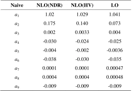
Table 2. Numerical values of αi in Naive Factorization

Naive NLO(NDR) NLO(HV) LO

a1 1.02 1.029 1.041

a2 0.175 0.140 0.073

a3 0.002 0.0033 0.004

a4 -0.030 -0.024 -0.025

a5 -0.004 -0.002 -0.0036

a6 -0.038 -0.030 -0.035

a7 0.0001 0.0001 0.00047

a8 0.0004 0.0004 0.00048

a9 -0.009 -0.009 -0.009

in which, P is the absolute value of the 3-momentum of the J /ψ (or the K−) in the B rest frame [14]. There are two serious problems with the naive factorization approximation. First, the Wilson coefficients Ci( )µ and hence ai are renormalization scale and

5

γ -scheme dependent, whereas the decay constants and form factors are not. Hence, the amplitude (13) is not physical. However, if we include the αs correction in the amplitudes, it turns out that the µ dependence of the Wilson coefficients is cancelled and the overall amplitude is insensitive to the renormalization scale. Second, nonfactorizable effects, which play an essential role in colour-suppressed modes, are not taken into account [16]. Nonfactorizable contributions at order of

s

α come from the radiative corrections of the operators

1, 4, 6, 8

O O O O and O10 and the relevant Feynman

diagrams are shown in Figure 1. The radiative corrections with a fermion loop do not contribute due to the color structure. For each operator O O O O1, 4, 6, 8 and

10

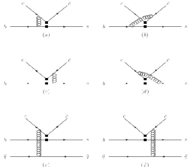
O if we add all the diagrams in Fig.1and symmetrize the result with respect to ξ↔ −1 ξ, the infrared divergence of each diagram will be canceled and the remaining amplitude will be infrared finite. One thing to note is that imaginary parts appear in the nonfactorizable contributions, which are due to the final-state interaction. The strong phase can be calculated in the QCD-improved factorization which is important in exploring the CP violation in nonleptonic decays. The two aforementioned difficulties for naive factorization are resolved in the QCD factorization approach in which the inclusion of vertex corrections and hard spectator interactions (see Fig. 1) yield [11, 15],

1

2 2 1

18 [

14 4

12 ln ]

s F

c c

I II b

C C

a C C

N N

f f

m α

π µ

 

= + + −_{ }

 

− + +

4

3 3 4

18 [

14 4

12 ln ]

s F

c c

I II b

C C

a C C

N N

f f

m α

π µ

 

= + + −_{ }

 

− + +

6

5 5 6

6 [

18 4

12 ln ]

s F

c c

I II b

C C

a C C

N N

f f

m α

π µ

 

= + − −_{ }

 

8

7 7 8

6 [

18 4

12 ln ]

s F

c c

I II b

C C

a C C

N N f f m α π µ   = + − −_{ }   − + + 10

9 9 10

18 [

14 4

12 ln ]

s F

c c

I II b

C C

a C C

N N f f m α π µ   = + + −_{ }   − + +

, (15)

where the upper entry of the matrix is evaluated in the naive dimension regularization (NDR) scheme and the lower entry is evaluated in the Hooft-Veltman (HV) renormalization scheme, 2

( 1) / (2 )

F c c

C = N − N , and c

N is the number of colors. Wilson coefficients are presented for leading order (LO) and next leading order (in NDR and HV scheme) in Table 1. The hard scattering functions fI arise from the vertex corrections, Figures 1(a)-1(d), while fII arsie from the hard spectator interactions Figures 1(e)-1(f). Formally, the coefficients ai are scale and

5

γ -scheme independent. The results for the hard scattering functions fI are (Tables 3, 4),

2 0 / 2 1 / ( ) ( ) BK J

I I BK I

J

F m

f f g

F m

ψ

ψ ′

= + (16)

where 1 / 2 0 2 2 2 2 2 ln

( ){ (3 2 8 )

1 (1 ) 1

3 1 8 2

( )

1 1 (1 ) [(1 (1 )] ln (3(1 ) 2 8 2 ln(1 )

)

1 (1 ) 1 (1 ) J I z f d z z

z z z

z z z z z

z z i

z z

ψ ξ ξ

ξϕ ξ ξ ξ

ξ ξ

ξ ξ

ξ ξ ξ

ξ ξ ξ ξ

ξ π ξ ξ ′ = + − − − − − + + − + − − − − − − + − + − − − + − − − −

∫

and 1 / 0

2 2 2

2

2

4 (2 1)

( ){ ln

(1 )(1 )

1 1

ln(1 ) (

[1 (1 )] (1 ) [1 (1 )]

8 2(1 2 )

) ln (1 )(1 ) (1 )(1 )

} [1 (1 )]

T I J g d z z z

z z z

z z

z z

z z z z

z i

z ψ

ξ ξ

ξϕ ξ ξ

ξ ξ

ξ ξ ξ

ξ ξ ξ ξ ξ ξ ξ π ξ − = − − + − + − − − − − − + − − + − − − − − − −

∫

In which, ( 2 2

/ /

J B

z =m _ψ m .ξ) is the momentum fraction of a c quark inside the J/ψ meson, and the asymptotic wave functions ( ( )ϕ ξ , T( )

ϕ ξ ) for the J /ψ meson are symmetric functions under ξ↔ −1 ξ. The asymptotic form of the distribution amplitudes ( )ϕ ξ and ϕ ξT( ) is the same. And

2 2 2

0 / /

2 2

1 /

( ) ( ) BK

J B J

BK

J B

F m m m

F m m

ψ ψ

ψ

− =

As for the hard scattering function fII that oraginates from spectator diagrams, we write [9],

2 3

II II II

f =f +f +…

where, the superscript denotes the twist dimension of LCDA. In the leading-twist order, we obtain (Tables 3, 4),

2 2

2 2

1 /

1 1 / 1 ( )

1

0 0 0

4 1 1 ( ) ( ) ( ) ( ) K B II BK J B

B J K

f f f

N F m m z

d d d

ψ

ψ π

π

ϕ ρ ϕ ξ ϕ η

ρ ξ η

ρ ξ η

=

−

∫

∫

∫

(17)

However, we shall see that the twist-2 nonfactorizable effects are numerically small; the predicted decay rate of B→J /ψK is too small by a factor of 7 ∼ 10. Therefore, it is inevitable that higher-twist effects, which are seemingly power- suppressed, play an essential role. Chirally enhanced corrections arise from twist-3 two-particle light-cone distribution amplitudes, whose normalization involves the quark

Figure 1. Vertex and spectator corrections to B→J/ψK

condensate (Table 3, 8). Consequently [9, 11],

2 3

2 2

1 /

1 1 1

/

1 2 3

0 0 0

2 4 ( ) ( ) ( ) ( ) ( ) 6(1 ) K B II BK

B J B

K

B J

f f f

m N F m m

d d d

z χ ψ ψ σ µ π ϕ η

ρ ξ η

ϕ ρ ϕ ξ

ρ ξ η

=

−

∫

∫

∫

(18)

The contributions to for example-B→Kπ- from the (S−P S)( +P) penguin operators are enhanced by the factor 2 2 2 12 (1) ( ) QCD K

b s u b b

m

O

m m m m m

χ

µ Λ

= ≈ ≈

+ (19)

Because it is difficult to fix the current masses of light quarks, we would like to take rK =rπ, which is proportional to the quark condensate. The logarithmic divergence of the η integral in (17) implies that the spectator interaction is dominated by soft gluon exchanges between the spectator quark and the charmed or anti-charmed quark of J/ψ. The twist-3 contribution involves the logarithmically divergent integral (M =K or π) [9],

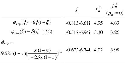
B→J/ψK Decay

Table 3. f_I , 2

II f , 3

II

f for B→J/ψK (q=s), µ =m_b

I

f fII2

3 ( 0) II H f ρ =

/ ( ) 6 (1 )

Jψ

ϕ ξ = ξ −ξ _{-0.813-6.61i 4.95 4.89}

/ ( ) ( 1 / 2)

Jψ

ϕ ξ =δ ξ− -0.517-6.94i 3.30 3.26

/

0.7

(1 ) 9.58 (1 )[ ]

1 2.8 (1 )

J x x x x x x ψ φ = − − − −

-0.672-6.74i 4.02 3.98

B→J/ψπ Decay

Table 4. fI ,

2

II f , 3

II

f for B→J/ψπ (q=d ), µ =mb

I

f 2

II f fII3

/ ( ) 6 (1 )

Jψ

ϕ ξ = ξ −ξ -0.813-6.61i 4.91 4.85

/ ( ) ( 1 / 2)

Jψ

ϕ ξ =δ ξ− -0.517-6.94i 3.27 3.24

/

0.7

(1 ) 9.58 (1 )[ ]

1 2.8 (1 )

J x x x x x x ψ φ = − − − −

-0.672-6.74i 3.99 3.94

1

0

(1 iH),

M B

H H

QCD m d

Ln eφ

η

ρ η

Χ ≡ = +

Λ

∫

0≤ρH ≤1 , −180〈φH〈180

(20) Because this divergence is associated with a soft interaction of the ejected meson with the spectator quark, the divergence arises specifically from the region,η ≈ ΛQCD /mB and therefore one expects that

( / )

M

H B QCD

X ≈Ln m Λ . The choice for the values of M

H

X introduces unavoidable model of dependence in the predictions [15, 16]. Here, we considered that

0, 0

H H

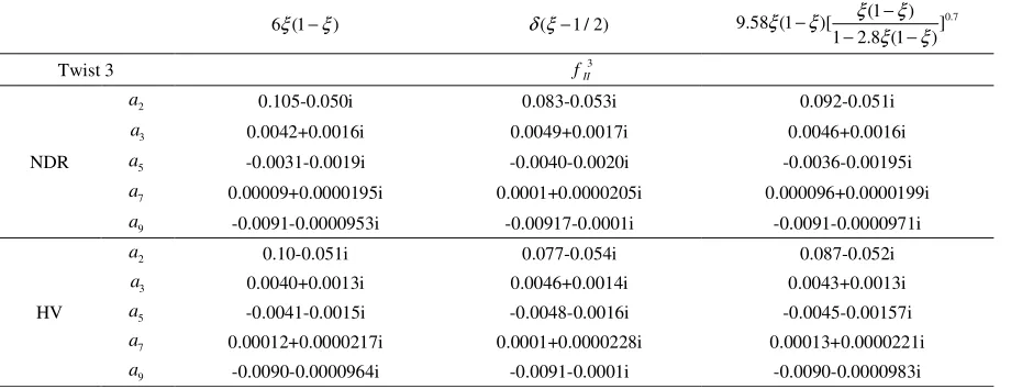
ρ = φ = and computed ai coefficients in QCD factorization (Tables 5, 6, 7, 8) by different 3-twist contributions.

D) Wave Functions of J/ψ, K, π, B

Consider the matrix’s element of nonlocal operators sandwiched between the vacuum and the vector meson [9, 17]:

5 5

5 5

/ ( ) (0) 0

{ / ( ) (0) 0 4

/ ( ) (0) 0 / ( ) (0) 0

/ ( ) (0) 0 1

/ ( ) (0) 0 } 2

a b

ab

J c x c

J c x c

N

J c x c

J c x c

J c x c

J c x c

α β µ µ µ µ µν µν βα ψ δ ψ

γ ψ γ

γ ψ γ

γ γ ψ γ γ

σ ψ σ

=

+

+

−

+

where a, b are color indices; α, β are indices for Dirac matrices. The leading-twist light-cone distribution amplitudes (LCDAs) of J /ψ are given by [9],

1

/ / /

0

/ ( ) ( ) (0) 0

( ) i P x

J J J

J P c x c

x

f m P d e

P x µ

ξ

ψ ψ µ ψ

ψ γ

ε

ξ ϕ ξ

∗ ⋅ = ⋅ ⋅

∫

1 / / 0

/ ( ) ( ) (0) 0

( ) ( )

T i P x T

J J

J P c x c

if P P d e

µν

ξ

ψ µ ν ν µ ψ

ψ σ

ε∗ ε∗ ξ ⋅ϕ ξ =

− −

∫

in which, ε∗

is the polarization vector of J/ψ; ξ is the light-cone momentum fraction of the c quark in J /ψ,

/

J

f _ψ and /

T J

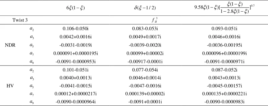
Table 5. Numerical value of ai for B→J /ψK (q=s), µ =mb , by using

2

II f

6 (1ξ −ξ) δ ξ( −1 / 2) 9.58 (1 )[ (1 ) ]0.7 1 2.8 (1 )

ξ ξ

ξ ξ

ξ ξ

− −

− −

Twist 3 fII2

NDR

2

a 0.0689-0.0505i 0.062-0.053i 0.067-0.051i

3

a 0.0054+0.0016i 0.0056+0.0017i 0.0054+0.0016i

5

a -0.0045-0.0019i -0.0047-0.0020i -0.0046-0.00195i

7

a 0.000105+0.0000196i 0.000108+0.0000205i 0.000105+0.0000199i

9

a -0.00919-0.0000953i -0.0092-0.0001i -0.0092-0.0000971i

HV

2

a 0.0629-0.0516i 0.056-0.054i 0.062-0.053i

3

a 0.00502+0.00135i 0.0052+0.0014i 0.0050+0.0014i

5

a -0.00523-0.00154i -0.0054-0.0016i -0.0053-0.00157i

7

a 0.000145+0.0000215i 0.000148+0.0000228i 0.000146+0.0000221i

9

a -0.00914-0.0000963i -0.0092-0.000101i -0.0091-0.0000983i

Table 6. Numerical value of a_i for B→J/ψK (q=s),µ =m_b by using 3

II f

6 (1ξ −ξ) δ ξ( −1 / 2) 9.58 (1 )[ (1 ) ]0.7 1 2.8 (1 )

ξ ξ

ξ ξ

ξ ξ

− −

− −

Twist 3 fII3

NDR

2

a 0.106-0.050i 0.083-0.053i 0.093-0.051i

3

a 0.0042+0.0016i 0.0049+0.0017i 0.0046+0.0016i

5

a -0.0031-0.0019i -0.0039-0.0020i -0.0036-0.00195i

7

a 0.000091+0.0000195i 0.00099+0.00002i 0.000096+0.0000199i

9

a -0.0091-0.0000953i -0.00917-0.0001i -0.0091-0.0000971i

HV

2

a 0.101-0.051i 0.077-0.054i 0.087-0.052i

3

a 0.0040+0.0013i 0.0046+0.0014i 0.0043+0.0013i

5

a -0.0041-0.0015i -0.0047-0.0016i -0.0045-0.00157i

7

a 0.00012+0.0000217i 0.000139+0.00002i 0.000135+0.0000221i

9

a -0.0090-0.0000964i -0.0091+0.0001i -0.0090-0.0000983i

1 1

/ /

0 0

( ) T ( ) 1

J J

dξϕ ψ ξ = dξϕ ψ ξ =

∫

∫

The leading-twist (twist-2) LCDAs of J /ψ can be expanded as [17],

2

/ 2

3

( ) 6 (1 )(1 [5(2 1) 1]) 2

Jψ a

ϕ ξ = ξ −ξ + ξ− −

2

/ 2

3

( ) 6 (1 )(1 [5(2 1) 1]) 2

T T

Jψ a

ϕ ξ = ξ −ξ + ξ− − (21)

where the parameters a2 and 2

T

a are defined by the matrix’s element of a twist-2 conformal operator with

conformal spin 3 [17]. While twist-2 DA ϕK can be expanded in terms of Gegenbauer polynomials C3/ 2:

2

2 3/ 2

2 2

1

( , )

6 (1 )(1 ( ) (2 1) K

K

n n

n

a C

ϕ η µ

η η µ η

∞

= =

− +

∑

− (22)

As before, η is the light-cone momentum fraction of the u quark in K−. Here, we consider the asymptotic function with the values of the Gegenbauer moments

2

K n

a to be an available from [18]. In the far ultraviolet µ → ∞, we have M 0

i

Table 7. Numerical value of a_i for B→J /ψπ (q=d ), µ =m_b by using 2

II f

6 (1ξ −ξ) δ ξ( −1 / 2) 9.58 (1 )[ (1 ) ]0.7 1 2.8 (1 )

ξ ξ

ξ ξ

ξ ξ

− −

− −

Twist 3 fII2

NDR

2

a 0.068-0.050i 0.058-0.053i 0.063-0.051i

3

a 0.0054+0.0016i 0.0057+0.0017i 0.0056+0.0016i

5

a -0.0045-0.0019i -0.0049-0.0020i -0.0047-0.0019i

7

a 0.000105+0.0000195i 0.000109+0.0000205i 0.000107+0.0000199i

9

a -0.0092-0.0000953i -0.0092-0.000100i -0.0092-0.0000971i

HV

2

a 0.062-0.051i 0.052-0.054i 0.056-0.052i

3

a 0.0050+0.0013i 0.0053+0.0014i 0.0051+0.0014i

5

a -0.0052-0.0015i -0.0055-0.0016i -0.0054-0.0016i

7

a 0.000145+0.0000217i 0.000150+0.0000228i 0.000148+0.0000221i

9

a -0.0091-0.0000964i -0.0091-0.000101i -0.0091-0.0000983i

Table 8. Numerical value of a_i for B→J/ψπ (q=d ),µ =m_b by using 3

II f

6 (1ξ −ξ) δ ξ( −1 / 2) _{9.58 (1 )[} (1 ) _]0.7

1 2.8 (1 )

ξ ξ

ξ ξ

ξ ξ

− −

− −

Twist 3 fII3

NDR

2

a 0.105-0.050i 0.083-0.053i 0.092-0.051i

3

a 0.0042+0.0016i 0.0049+0.0017i 0.0046+0.0016i

5

a -0.0031-0.0019i -0.0040-0.0020i -0.0036-0.00195i

7

a 0.00009+0.0000195i 0.0001+0.0000205i 0.000096+0.0000199i

9

a -0.0091-0.0000953i -0.00917-0.0001i -0.0091-0.0000971i

HV

2

a 0.10-0.051i 0.077-0.054i 0.087-0.052i

3

a 0.0040+0.0013i 0.0046+0.0014i 0.0043+0.0013i

5

a -0.0041-0.0015i -0.0048-0.0016i -0.0045-0.00157i

7

a 0.00012+0.0000217i 0.0001+0.0000228i 0.00013+0.0000221i

9

a -0.0090-0.0000964i -0.0091-0.0001i -0.0090-0.0000983i

scale of QCD; we expect the Gegenbauer moments M i α to be small. The asymptotic form of the distribution amplitudes ϕ ξ( ) and _{ϕ ξ}T( )

is the same, which is given as _{ϕ ξ}( ) _{ϕ ξ}T( ) 6 (1_{ξ ξ})

= = − . In the numerical analysis, we also consider the wave function of the form: ( ) T( ) ( 1/2)

ϕ ξ ϕ ξ δ ξ= = − , ( ) T( ) 9.58 (1 )

ϕ ξ ϕ ξ= = ξ −ξ

0.7

(1 )

[ ]

1 2.8 (1 )

ξ ξ

ξ ξ

− ×

− − [19]. Twist-3 LCDAs, K

p

ϕ K

σ

ϕ of the kaon are defined in the pseudoscalar and tensor matrix’s elements. They can be expanded in terms of Gegenbauer polynominals:

1/ 2 1/ 2

2 4

( ) 1 ( ) ( ) K

p aC bC

ϕ η = + η + η +…

3/ 2 2

( ) 6 (1 )(1 ( ) )

K

dC

σ

ϕ η = η −η + η +… (23)

in which can we find the coefficients a, b, d in [18]. Twist-3 DAs of pseudoscalar mesons are associated with a chiral enhancement factor µχ. We take its asymptotic form, Then we apply ϕ ησK( )=6 (1η −η)

and K( ) 1 p

ϕ η = . We find that the twist-3 kaon LCDA K

σ

ϕ contributes to spectator diagrams in B→J /ψK decay. For the B meson, we use [20],

2 2 2

1

1

( ) (1 ) exp[ ( ) ] 2

B B

B

B m

N ρ

ϕ ρ ρ ρ

ω

= − − (24)

constant, 1

0ϕ ξB( )dξ=1

∫

. This B meson wave function corresponds to λ =B 300MeV , which is defined by

1 0 ( ) B B B m

dξ ξ

ξ λ

Φ ≡

∫

. This can be understood since the B meson wave function is peaked at small ξ: It is of the order of mB /ΛQCD at ρ≈ ΛQCD /mB. Hence, the integral over ϕ ρB( ) /ρ produces a mB /ΛQCD term [9,11].

E) Form Factors

The form factors are parametrized as [14],

2 2 2 1 2 2 2 2 0 2 (( ) ) ( ) ( ) B P B P B P

P J B p p

m m

q F q

q

m m

q F q q µ µ µ µ = + − − − + B p

q=p −p . The 2

q behavior of B-to-light form factors in the LCSR analysis is parametrized as [22]:

2 2 2 2 1,0 2 1,0 ₂ (0) ( )

1 ( )

B B

q q

F m F m

F

F q

a b

=

− + (25)

where the relevant fitted parameters aF and bF in Table 9 (q2 =mJ2_/ψ) and the momentum dependence of form factors is given by [22],

2 2

2 2

0 2 2 2 2 1

5.4

( ) 0.28( ) ( )

5.4

B B

B

q

F q F q

q m m

π π π = − + − − , 2 2 2 2

0 2 2 2 2 1

5.8

( ) 0.32( ) ( )

5.8

BK BK

B K

q

F q F q

q m m

= − +

− − , (26)

In this section, form factors are calculated by (25).

F) Branching Ratio

The decay rate is simply given by

2

1 2

16 B eff

S

M M H B

m π Γ =

where S =1 / 2, if M1 and M2 are identical, and S =1

otherwise [8]. Also the decay rates for B→M M1 2 are

given by

(

)

(

)

2

1 2 ₈ 2 1 2

s

c s

B p

B M M M B M M

m

π

Γ → = → (27)

where

1 2 1 2

2 2 2 2

( ( ) )( ( ) )

2 c

B M M B M M

B p

m m m m m m

m =

− + − − (28)

is the c m. . momentum of the decay particles [21]. We assume that in the limit, in which mb goes to infinity,

/

J

m ψ is heavy enough to regard the size of the J/ψ meson as small, but light enough to employ the leading-twist light-cone wave function for J/ψ. Then,

/ 2

c B

P =m and pB.ε mB2 / 2mJ/ψ ∗₌

.The branching ratio is given by

(

)

2

1 2 2

1 8 c i B tot B p

R B M M M

m

τ π Γ

Β → = =

Γ (29)

where τ =B /Γtot=1.638 ps, Γtot=(4.2±0.3)×10-13 [30].

Results

For numerical analysis, we use the following input parameters [9, 11]:

4.4 b

m = GeV , mc =1.5GeV , mB =5.28GeV ,

/ 3.1

J

m ψ = GeV , fJ/ψ =405MeV , fB =190MeV , 160

K

f = MeV , fπ =133MeV , ΛQCD =300MeV ,

300

B MeV

λ ≈ , α µ =s( mb)≈0.2, and [21, 23, 24],

2 1 ( / ) 0.7

B K J

F → m _ψ = , 2

0 ( / ) 0.418

B K J

F → m _ψ = , 2

1 ( / )

B J

F →π m _ψ

= 0.587 , 2

0 ( / ) 0.351

B J

F π m ψ

→ = , 2 1 4 2 3 F N C N −

= = , GF=

5

1.166 10× − , VCKM =

(1.2 0.08)

(1.2 0.08) (1.2 0.08)

(1.2 0.08) (1.2 0.08) 0.9603 0.223 0.0037

0.225 0.0001 0.969 0.00003 0.041 0.009 0.0035 0.040 0.0008 0.989

i i i i i e e e e e − ± ± ± ± ±     − − −    _{− − −}    ,

|V Vcb cs ∗

|=0.039, |V Vtb ts ∗

|=0.041, |V Vcb cd ∗

|=0.009, |V Vtb td

∗_{|=0.0319−0.014i,}

Since there are no mixing effects present in the charged B-meson system, non-vanishing CP asymmetries of the kind

( ) ( )

( )

( ) ( )

CP

B f B f

A B f

B f B f

+ −

+

+ −

Γ → − Γ →

→ ≡

would give us unambiguous evidence for “direct” CP violation in the B system; The CP asymmetries (30) arise from the interference between decay amplitudes with both different violating weak and different CP-conserving strong phases. In the SM, the weak phases are related to the phases of the CKM matrix elements, whereas the strong phases are induced by final-stateinteraction processes. In general, the strong phases introduce severe theoretical uncertainties into the calculation of A_CP(B+→f ), thereby it destroys the clean relation to the CP-violating weak phases. However, there is an important tool to overcome these problems, which is provided by amplitude relations between certain nonleptonic B decays. For the charged B meson decays, the direct CP-violating asymmetries

dir CP

A can be defined as usual. For B+ J/ψK+

→

decay, there is no direct CP violation, since there is no weak phase appeared in their decay amplitude [25].

( / ) 0.017 0.016

dir CP

A B+ J ψK+

→ = ±

( / ) 0.09 0.08

dir CP

A B+ J ψπ+

→ = − ±

In this scheme in the standard model, there is no contribution to CP asymmetry in the decay amplitude since the CKM matrix elements involved here are all real. The CP asymmetry totally comes from 0 0

B −B

mixing. For the 0

1 2

B →M M decays, because these decays are neutral B meson decays, we should consider the effects of 0 0

B −B mixing. In the case of B →J/ψK , we have to deal both with current–current, i.e. tree-diagram-like, and with penguin contributions. For the

0

B decay, the CP asymmetry is time dependent [27].

( ) dirsin( ) mix cos( )

CP CP CP

A t =A ∆mt +A ∆mt (31) The direct and mixing induced CP-violating asymmetries dir

CP

A and mix CP

A can be written as [27],

2

2 2

1 2 sin sin 1 2 cos cos 1

CP dir CP

CP

r A

r r

λ δ γ

δ γ

λ

−

= =

+ +

+

2

2

2

2 Im( ) 1

sin 2 2 cos sin(2 ) sin 2( ) 1 2 cos cos

mix CP

CP

CP A

r r

r r

λ λ

β δ β γ β γ

δ γ

= =

+

+ + + +

−

+ +

(32)

where γ β δ, , are used in the Wolfenstein approximation. The CP-violating parameter λCP is [27],

Form Factors

Table 9. Values of a_F and b_F

bF aF

F(0)

0.27 1.35

0.3±0.04

F+π

0.62 0.39

0.3±0.04

0

Fπ

0.26 1.34

0.3±0.04

T Fπ

0.35 1.37

0.35±0.05

K F+

0.41 0.40

0.035±0.05

0

K F

0.37 1.37

0.36±0.05

K T F

CP asymmetry

Table 10. Determination of weak phase β through mixing-induced CP asymmetry

(deg) β ββ

β SJ/ψψψψK SJ/ψπψπψπψπ

Table 11. Decay rates in Naïve Factorization and QCD Factorization for B→J/ψK , (GeV), (µ =m_b)

(LO)

Γ Γ(NLO)

(NDR)

(NLO)

Γ

(HV)

NF 1.61×10-16 _8.46×10-16 _5.32×10-16

QCDF

/ ( ) 6 (1 )

Jψ

ϕ ξ = ξ −ξ

2

II f

2.07×10-16 1.92×10-16

/ ( ) ( 1 / 2)

Jψ

ϕ ξ =δ ξ− 1.37×10-16 _1.31×10-16

/

0.7

(1 ) 9.58 (1 )[ ]

1 2.8 (1 )

J

x x

x x

x x

ψ

φ =

− −

− −

2.01×10-16 1.92×10-16

/ ( ) 6 (1 )

Jψ

ϕ ξ = ξ −ξ

3

II f

3.77×10-16 3.59×10-16

/ ( ) ( 1 / 2)

Jψ

ϕ ξ =δ ξ− 2.71×10-16 2.52×10-16

/

0.7

(1 ) 9.58 (1 )[ ]

1 2.8 (1 )

J

x x

x x

x x

ψ

φ =

− −

− −

3.12×10-16 2.91×10-16

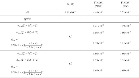
Table 12. Decay rates in Naïve Factorization and QCD Factorization for B→J /ψπ.(GeV), (µ =m_b)

(LO)

Γ Γ(NLO)

(NDR)

(NLO)

Γ

(HV)

NF 1.02×10-17 4.44×10-17 2.71×10-17

QCDF

/ ( ) 6 (1 )

Jψ

ϕ ξ = ξ −ξ

2

II f

1.21×10-17 _1.19×10-17

/ ( ) ( 1 / 2)

Jψ

ϕ ξ =δ ξ− 1.08×10-17 1.06×10-17

/

0.7

(1 ) 9.58 (1 )[ ]

1 2.8 (1 )

J

x x

x x

x x

ψ

φ =

− −

− −

1.13×10-17 1.11×10-17

/ ( ) 6 (1 )

Jψ

ϕ ξ = ξ −ξ

3

II f

1.96×10-17 1.96×10-17

/ ( ) ( 1 / 2)

Jψ

ϕ ξ =δ ξ− 1.53×10-17 1.51×10-17

/

0.7

(1 ) 9.58 (1 )[ ]

1 2.8 (1 )

J

x x

x x

x x

ψ

φ =

− −

− −

Table 13. Branching ratios in Naïve Factorization and QCD Factorization for, B→J/ψK, (GeV), (µ =m_b)

( )

BR LO BR NLO( ) (NDR) BR NLO( ) (HV)

NF 0.3

0.3

3.8+− ×10

-4 1.6

1.3

20.1+− ×10

-4 1.0

0.8

12.6+− ×10

-4

QCDF

/ ( ) 6 (1 )

Jψ

ϕ ξ = ξ −ξ

2

II f

0.4 0.3

4.9+ − ×10

-4 0.4

0.3

4.5+ − ×10

-4

/ ( ) ( 1 / 2)

Jψ

ϕ ξ =δ ξ− 0.3

0.2

3.2+− ×10

-4 0.2

0.2

3.1+− ×10

-4

/

0.7

(1 ) 9.58 (1 )[ ]

1 2.8 (1 )

J

x x

x x

x x

ψ

φ =

− −

− −

0.4 0.3

4.7+ − ×10

-4 0.4

0.3

4.5+ − ×10

-4

/ ( ) 6 (1 )

Jψ

ϕ ξ = ξ −ξ

3

II f

0.7 0.6

8.9+− ×10

-4 0.7

0.6

8.5+− ×10

-4

/ ( ) ( 1 / 2)

Jψ

ϕ ξ =δ ξ− 0.5

0.4

6.4+− ×10

-4 0.4

0.4

6.0+− ×10

-4

/

0.7

(1 ) 9.58 (1 )[ ]

1 2.8 (1 )

J

x x

x x

x x

ψ

φ =

− −

− −

0.6 0.5

7.4+− ×10

-4 0.5

0.5

6.9+− ×10

-4

Exp [25] (10.07± 0.35)×10−4

Table 14. Branching ratios in Naïve Factorization and QCD Factorization for B→J/ψπ,(GeV), (µ =m_b)

( )

BR LO BR NLO( ) (NDR) BR NLO( ) (HV)

NF 0.240.020.02

+ − ×10

-4 0.01

0.01

0.10+ − ×10

-4 0.05

0.04

0.64+ − ×10

-4

QCDF

/ ( ) 6 (1 )

Jψ

ϕ ξ = ξ −ξ

2

II f

0.03 0.02

0.28+− ×10

-4 0.02

0.02

0.28+− ×10

-4

/ ( ) ( 1 / 2)

Jψ

ϕ ξ =δ ξ− 0.02

0.01

0.25+ − ×10

-4 0.02

0.02

0.25+ − ×10

-4

/

0.7

(1 ) 9.58 (1 )[ ]

1 2.8 (1 )

J

x x

x x

x x

ψ

φ =

− −

− −

0.02 0.01

0.26+− ×10

-4 0.02

0.02

0.26+− ×10

-4

/ ( ) 6 (1 )

Jψ

ϕ ξ = ξ −ξ

3

II f

0.04 0.03

0.46+ − ×10

-4 0.04

0.03

0.46+ − ×10

-4

/ ( ) ( 1 / 2)

Jψ

ϕ ξ =δ ξ− 0.03

0.02

0.36+− ×10

-4 0.03

0.02

0.35+− ×10

-4

/

0.7

(1 ) 9.58 (1 )[ ]

1 2.8 (1 )

J

x x

x x

x x

ψ

φ =

− −

− −

0.03 0.03

0.40+ − ×10

-4 0.03

0.03

0.40+ − ×10

-4

0 2

0

eff i

CP f

eff

f H B

e

f H B

β

λ η −

= (33)

where ηf is the CP-eigenvalue of the final states and ( ) / ( )

r=P penguin T tree . It only keeps linear terms in

r,

2 sin sin

dir CP

C ≡A ≈ r δ γ,

sin 2 2 cos 2 cos sin S mix

CP

S A β r β δ γ

∆

≡ ≈ − −

In b→ccs quark-level decays, the time-dependent CP violation parameters measured from the interference between decays with and without mixing are

sin 2

ccs CP

S = −η β and Cccs =0, to a very good approximation. The theoretically cleanest case if

/

B →J ψK , where

2 /

i

J K e

β ψ

λ ₌ −

∓ (34)

and so

/

Imλ_JψK = ±sin 2β

Then

( / ) sin(2 )

mix CP

A B →J ψK = β

0

( / ) sin( 2 )

mix CP

A B →J ψπ = − β

,

( ) sin(2 ) cos( )

CP d s

A t = ± β ∆m t (35)

One more important implication of the SM is [26, 27, 28, 29],

( / ) 0 ( / )

dir

CP d CP

A B J ψK A B+ J ψK+

→ ≈ ≈ →

This theoretical expectation agrees well with the data [25],

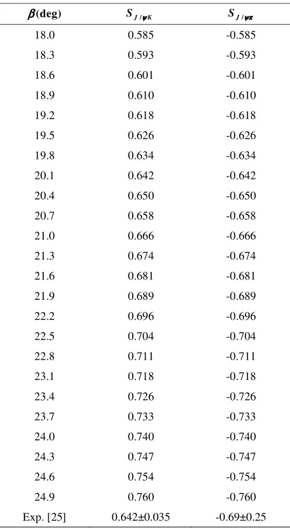
0 0

( / ) 0.018 0.025

dir CP

A B →J ψK = − ±

0 0

( / ) 0.11 0.25

dir CP

A B →J ψπ = − ±

We computed sin(2 )β [18≤β≤24.9] in Tablel 10 and compared it with experimental data, which are for

0 0

/

B →J ψK in β=20.1 and for 0 0 /

B →J ψπ in 22.2

β= .

Discussion

The hadronic decays B→J /ψK( )π are interesting because experimentally they are the only

color-suppressed modes which have been measured, and theoretically they are calculable by QCD factorization, even the emitted meson J/ψ is heavy. We computed

i

a coefficients in Naïve factorization (Table 2) and in QCD factorization (Tables 5, 6, 7, and 8) by different 3-twist contributions, and then we obtained decay rates (Tables 11, 12) and branching ratios for two decays (Tables 13, 14). We compared branching ratios in Tables 13, 14 which, for /

6 (1 )

Jψ

ϕ = ξ −ξ function, is in agreement with experiments.

• In the colour suppressed B→J /ψK and J/ψπ

decays, non-factorizable contribution is more important. Our result on the color suppressed

/

B →J ψK and B→J/ψπ decays is still sensitive to the values of both of 2

1 ( / )

B J F →π m _ψ [or

2

1 ( / )

B K J

F m ψ

→

].

• We considered coefficients in µ=mb and three functions for J/ψ, that numerical results are better for /

6 (1 )

Jψ

ϕ = ξ −ξ . Also, we assumed ρH =0. • To leading-twist contributions from the light-cone

distribution amplitudes (LCDAs) of the mesons, vertex corrections and hard spectator interactions, which include mc effects, imply result in Tabls 3, 8. Hence, the predicted branching ratio is too small by a factor of 5; the nonfactorizable corrections to naive factorization to leading-twist order are small. • We study the twist-3 effects due to the kaon. The

prediction BR B( →J/ψK( ))π is in agreement with

experiments; 4

( / ) (10.07 0.35) 10

BR B_→J ψK _{= ± ×} −

4

( / ) (0.49 0.06) 10

BR B J ψπ −

→ = ± × [25].

References

1.Naboulsi R. Theory of Hadronic Decays in B Meson System in the SM. arXiv: [hep-ph] 0304039 (2003). 2.Beneke M. Conceptual aspects of QCD factorization in

hadronic B decays. J. Phys. G: Nucl. Part. Phys. 27: 1069-1081(2001).

3.Bauer M., Stech B., Wirbel M. Exclusive Semileptonic Decays of Heavy Mesons. Z. Phys. C 29: 637-649 (1985); Z. Phys. C 34: 103-118 (1987).

4.Neubert M., Stech B. Non-leptonic Weak Decays of B mesons. Adv.Ser.Direct. High Energy Phys. 15: 294-312 (1998).

5.Reader C., Isgur N. Factorization and heavy-quark symmetry in hadronic B-meson decays. Phys. Rev. D 47: 1007-1019 (1993).

6.Beneke M., Buchalla G., Neubert M., Sachrajda C. T. QCD Factorization for B→ππ Decays. Phys. Rev. Lett. 83: 1914-1928 (1999).

8.Beneke M., Neubert G. QCD factorization for B→PP and B→PV decays. Nucl.Phys. B675: 333-351 (2003). 9.Chay J., Kim C. Analysis of the QCD-improved facto-rization in B→J /ψK . arXiv:[hep-ph] 0009244 (2000). 10.Leitner O., Gue X. H., Thomas A. W. Direct CP violation,

Branching ratios and form factors B→π, B→K in B decays. J. Phys. G: Nucl. Part. Phys. 31, 199-215 (2005). 11.Cheng H. Y., Yang K. C. B→J/ψK Decays in QCD

Factorization. Phys. Rev. D63: 074011-074026 (2001). 12.Muta T., Sugamoto A., Yang M. Z. Decays in the QCD

Improved Factorization Approach. Phys. Rev. D62: 094020-094036 (2000). Yang D. D., Zhu G. D. Analysis of the Decays and with QCD Factorization in the Heavy Quark Limit. arXiv:[hep-ph]0008216 (2000).

13.Politzer H. D., Wise M. B. Kaon condensation in nuclear matter. Phys. Lett. B257: 399-417 (1991).

14.Ali A., Greub C. An analysis of two-body non-leptonic B decays involving light mesons in Standard Model. Phys.Rev. D57: 2996-3014 (1998).

15.Cheng H. Y. Exclusive and Semi-inclusive B Decays in QCD Factorization. arXiv:[hep-ph]0108621 (2001). 16.Virto J. Topics In Hadronic B Decays.

arXiv:[hep-ph]0712.3367v2 (2007).

17.Ball P., Braun V.M. Higher twist distribution amplitudes of vector mesons in QCD. Nucl. Phys. B543: 201-217 (1999). 18.Ball P. Theorical update of psedoscalar mesons

distribution amplitudes of higher twist: The nonsinglet Case. JHEP, 9901: 010-022 (1999).

19.Li J. W., Du D. S., Wu X. Y. Probing new physics in

0

/

B→J ψπ decay. arXiv: [hep-ph] 0904.1304v1(2009). 20.Keum Y. Y., Li H. N., Sanda A. I. Penguin Enhancement

and B→πK _{decays in perturbative QCD. Phys. Rev.} D63: 054008-054022 (2001).

21.Cheng H. Y., Yang, K. C. Updated Analysis of a₁ and a₂ in Hadronic Two-body Decays of B Mesons. arXiv:[hep-ph]9811249v2 (1999).

22.Ball P., Braun V. M. Exclusive semileptonic and rare B meson decays in QCD. Phys. Rev. D 58: 094016-094029 (1998). Ball P. B→K and B→π transitions from QCD sum rules on the light-cone. JHEP, 9809: 005-013 (1998). 23.Ball P. B Decays into Light Mesons. arXiv: [hep-ph]

9803501 (1998).

24.Terasaki K. Non-factorizable contributions in B decays revisited. Int. J. Theor. Phys.Group Theor.Nonlin. Opt. 8: 55-69 (2002).

25.Particle Data Group, Amsler, C. et al., Physics Letters B667: 1-28 (2008).

26.Gronau M., Rosner J. L. Small amplitude effects in

0

B _→D D+ − _{and related decays. Phys.Rev.D78:}

033011-033025 (2008).

27.Liu X., Zhang Z. Q., Xiao Z. J. B→( /J ψ η, c)K decays in the perturbative QCD approach. arXiv:[hep-ph]0901.0165v3 (2009).

28.Boos H., Mannel T., Reuter J. The Gold-plated mode revisited: sin 2β and B0→J/ψK in the Standard Model. Phys.Rev. D70: 036006-036021 (2004).

29.Buchalla G., Komatsubara T. K., Muheim F., Silvestrini L. B, D and K decays. Eur. Phys. J. C57: 309-326 (2008). 30.Cottingham W. N., Mehrban H., Whittingham I. B.