A new stochastic mixed integer programming to design integrated cellular manufacturing system: A supply chain framework Pages 563-574 Download PDF

(1)

International Journal of Industrial Engineering Computations 2 (2011) 563–574

Contents lists available at GrowingScience

International Journal of Industrial Engineering Computations

homepage: www.GrowingScience.com/ijiec

A new stochastic mixed integer programming to design integrated cellular manufacturing system: A supply chain framework

Vahid Reza Ghezavatia*

a_{Department of Industrial Engineering, Islamic Azad University, South Tehran Branch, Tehran, Iran}

A R T I C L E I N F O A B S T R A C T

Article history:

Received 02 January 2011 Received in revised form 10 March 2011

Accepted 12 March 2011 Available online 15 March 2011

This research defines a new application of mathematical modeling to design a cellular manufacturing system integrated with group scheduling and layout aspects in an uncertain decision space under a supply chain characteristics. The aim is to present a mixed integer programming (MIP) which optimizes cell formation, scheduling and layout decisions, concurrently where the suppliers are required to operate exceptional products. For this purpose, the time in which parts need to be operated on machines and also products' demand are uncertain and explained by set of scenarios. This model tries to optimize expected holding cost and the costs regarded to the suppliers network in a supply chain in order to outsource exceptional operations. Scheduling decisions in a cellular manufacturing framework is treated as group scheduling problem, which assumes that all parts in a part group are operated in the same cell and no inter-cellular transfer is required. An efficient hybrid method made of genetic algorithm (GA) and simulated annealing (SA) will be proposed to solve such a complex problem under an optimization rule as a sub-ordinate section. This integrative combination algorithm is compared with global solutions and also, a benchmark heuristic algorithm introduced in the literature. Finally, performance of the algorithm will be verified through some test problems.

Cellular manufacturing Stochastic MIP Uncertain processing time Supplier network

1. Introduction

(2)

where both machines and workers can improve their performance by repeating the production operations. Therefore, the actual processing time of a job is shorter if it is scheduled later in a sequence. This phenomenon is introduced as the “learning effect” in the literature (Badiru, 1992). Therefore, developing integrated models for CMS under uncertainty belongs to a relatively new class of CMS and tactical problems.

In any manufacturing environment, suppliers or supply chain network structures play vital role in producing different products. A manufacturer can decide whether the operations are completed inside the manufacturing system or they have to be outsourced to the suppliers in a supply chain network. Thus, suppliers can decide on the characteristics of operation processes, which are not completed inside the system.

For each stochastic programming (SP) problem applying uncertain parameters, one must decide which decision variables are considered during the first stage and which ones are taken into account during the second stage where the uncertainty has been resolved (Snyder, 2006; Ghezavati, 2009). In stochastic CMS problem, cell formation (CF) decisions variables must be made, while scheduling decisions are determined in future after the realization of uncertainty occurs.

The CMS problem with uncertain parameters can classified as (1) Fuzzy approach, (2) Stochastic optimization and (3) heuristic procedures. There are many studies in CMS problems where uncertain parameters are considered in fuzzy form. Papaioannou and Wilson (2008) proposed CMS problems analysis where coefficients in the objective function and constraints are considered as fuzzy values. Shanker and Vrat (1999) used fuzzy approach in order to forecast future variations of formulation process. Szwarc et al. (1999) considered uncertainty in machines’ capacity located in cells for a CMS problem and solved the resulted problem formulation using fuzzy approach.

Stochastic programming (SP) is applicable in many areas of production planning. However, in CMS problem, this approach is usually applicable just for handling changes in demand while there are many other factors, which are also stochastic. Some researches deal with aggregated CMS problem with tactical decisions such as production planning where demand is stochastic (Hurley & Whybark, 1999). In addition, there are some other studies to consider layout decisions with stochastic CMS demand, concurrently (Tavakkoli-Moghaddam, 2007). Balakrishnan and Cheng (2007) focused on CMS problem in dynamic situations and stochastic demand in which demand is changed from one period to another one. Kuroda & Tomita (2005) considered CMS problem as a probabilistic programming in which the time between two sequence failures follows exponential distribution. In addition, Markov chain and queuing theory were also applied in some studies to handle uncertainty in machines’ availability (Gupta & Kavusturucu, 1998).

Aggregated CMS problems can be solved using different techniques such as heuristic or meta-heuristic approaches. Balakrishnan and Cheng (2005), for instance, proposed meta-heuristic method to solve aggregated CMS problems. Andres (2007) proposed heuristic algorithms for CMS problems with uncertainty in processing time. Cell formation was also studied in an integrated form with scheduling (Solimanpur, 2004; Lockwood et al., 2000) and in an integration of exceptional elements with CF decisions (Tsai et al., 1997; Mahdavi et al., 2007). During the past two decades, there has been a great effort on applying meta-heuristics and heuristics methods to solve large-scale CMS problems which are also practical and appealing for real-world case studies (Wu et al., 2006; Venkataramanaiah, 2007).

(3)

satisfactory well under all scenarios. In some applications, scenario planning replaces estimating as a way to assess trends and possible changes in the business environment.

2. Formal description of the problem and of the mathematical model

2.1Formal description of the problem

The integrated cellular manufacturing problem consists of classical cell formation objectives, scheduling considerations and also, layout aspects in a supply chain framework. The classical cellular manufacturing problem aims to set cell of machines and part families to form independent cells with minimum number of inter-cell and intra-cell number movements without suppliers' considerations. Within a manufacturing cell, it is critical to integrate strategic objectives with the operational and tactical ones in an uncertain decision space. This is because of the fact that in real-world application design of products, customers' expectations, products' life cycles and market characteristics can be fluctuated during a production plan. Thus, decisions associated with each manufacturing plan must be made under uncertain conditions. Scheduling problem in a cellular manufacturing environment is formulated as group scheduling problem, which assumes that all part families are processed in the same cell and no inter-cellular transfers are needed. Layout consideration is another tactical aspect, which can be optimized during design stage and also, has direct impact on the transportation costs arisen in a manufacturing systems. The impact of both above objectives will be surveyed through a supply chain network design. There are three different objective associated with most of CMS problems. The first objective is to optimize under utilization and similarities objectives. The second objective is to optimize scheduling costs, which is measured by the flow time criterion. The third objective is to find the best location of machines in each work cell in order to optimize intra-cell movements. Uncertainty in decision space is considered as some discrete scenarios and thus scenario based planning approach will be applied to formulate mathematical model. In addition, stochastic optimization framework can be applied to formulate the proposed model.

Scenario based planning is a method in which decision makers come up with uncertainty by indicating a number of possible future states. The goal is to find solutions, which perform well under all scenarios. In some cases, scenario planning replaces predicting as a way to assess trends and potential modifications in the industry environment (Mobasheri et al., 2989). Companies can thus develop strategic responses to a range of environmental adjustments, more adequately preparing themselves for the uncertain future. Under such conditions, scenarios are qualitative descriptions of possible future states, consequences from the present state with the consideration of potential key industry events. In other cases, scenario planning is used as a tool for modeling and solving specific operational problems (Mulvey, 1996). While scenarios here also depict a range of future circumstances, they also represent quantitative descriptions of different values.

It is assumed that processing time of parts on machines and product demand are uncertain described by discrete scenarios. There are a set of scenarios where each occurs with probabilityps. Since there

are multiple scenarios for any CMS problem, group scheduling decisions must be made under each scenario. The primary strategy in group scheduling is to minimize the expected waiting costs (leads to holding cost) in cells for parts under all scenarios. So, in this formulation, total expected cost includes expected holding costs, cost of subcontracting exceptional elements and transportation between machines based on the location of machines. The following assumptions are considered in a problem:

1) Cell formation, scheduling and layout considerations are integrated in a single mathematical model. 2) Stochastic optimization framework is applied to formulate the proposed problem.

3) The location of all suppliers is assumed to be fixed in supply chain network.

4) The outsourcing costs consist of all cost regarded to the suppliers such as operating cost, transportation cost and the costs regarded to the suppliers' location.

5) All parts are available to be operated at the beginning of the planning period.

(4)

9) Processing time for each part on each machine is stochastic and described by set of discrete scenarios where probability of occurring each scenarios isps.

10)Each part has a number of operations which is determined by machine-part matrix. 11)Cost of sub-contracting and underutilization is known and deterministic.

2.2 Description of the mathematical model

We use the following notation:

Sets

M Set of parts N Set of machines C Set of cells

S Set of scenarios L Set of locations Parameters

1 = ij

a If part i require to be processed on machine j, 0 otherwise,

1

,j′=

ij

b If operation j' of part i is performed after completion of operation j, 0 otherwise,

ij

OC Outsourcing cost of operation j for part i to the suppliers in a supply chain network,

max

M Maximum number of machines permitted in a cell,

is

d Amount of demand of product i under scenario s,

u

C Maximum number of cells permitted to be formed,

s

p Probability of scenario s occurs,

ijs

t Processing time for part i on machine j in scenario s,

p p

mt , ′ The time needed to move from location p to location p',

T Holding cost per unit of time for parts waiting in cells,

Decision variables

1 = ik

x If part i is processed in cell k, 0 otherwise,

1 = jk

y If machine j is assigned to cell k, 0 otherwise,

1

,

,ps =

j

z If machine j is located in pth location under scenario s, 0 otherwise,

s i

g _, The time in which operation of part i in cell k starts,

s i

tp_, Total processing time of part i under scenario s,

1

,i′=

i

N If operations of part i starts before operations of part i',

Mathematical model

∑

∈ ∈ × × ⎟⎟ ⎠ ⎞ ⎜⎜ ⎝ ⎛ + × = S s is M i is is

s g tp h d

p f₁

∑

∑∑∑

∈ ∈ ∈ ∈ ⎟ ⎟ ⎠ ⎞ ⎜ ⎜ ⎝ ⎛ − × × × × = S

s k Cj Ni M

jk ik ij is ij

s OC d a x y

p

f₂ (1 )

2 1

min F = f + f (1)

subject to:

i x

C k

ik = ∀

∑

∈ 1 (2) j y C k

jk = ∀

∑

∈

(5)

s j z L p s p

j, , =1 ∀,

∑

∈ (4) p s k y z N j jk s p

j, , × ≤1 ∀ , ,

∑

∈ (5) s i mt z z b y x t tp N j p p s p j N

j j Np Lp L

s p j j j i C k jk ik ijs

is ,' ,' , ' 0 ,

' ' , , , , _⎟⎟= ∀ ⎠ ⎞ ⎜ ⎜ ⎝ ⎛ × × × + × × −

∑

∑ ∑∑ ∑

∈ ∈ ∈ ∈ ∈ ′ ∈ (6) s i i x x M tp g M N

g_is + _i_,_i_'× ≥ _i_'_s + _i_'_s − × _ik ×(1− _i_,'_k) ∀, ,' (7)

k s i i x x M tp g M N

g_i_'_s +(1− _i_,_i_')× ≥ _is + _is − × _ik×(1− _i_,'_k) ∀, ,' , (8)

Max N j jk M y ≤

∑

∈ (9) 0 , } 1 , 0 { , ,

, _jk _j_,_p_,_s _i_,_i_'∈ _is _is ≥

ik y z N g tp

x (10)

The objective f1 determines expected holding cost through multiplying probability of scenario by the total time, where a process is completed. The function f2 computes total expected cost associated with the outsourcing operations. The objective function (1) denotes optimization criterion. Set constraint (2) says that each part must be assigned to a single cell. Set constraint (3) states that each machine can be assigned only to one cell. Set constraint (4) ensures that each machine must be allocated to one location under each scenario. Set constraint (5) specifies that at most one machine can be allocated to each location in each cell. Set constraint (6) computes total operation time for each part under each scenario, which consists of processing time and intra-cell transportation time. Constraints (7) and (8) ensure that a cell cannot process more than one product at the same time if both parts i and i' are located in the same cell. Constraint (10) determines the maximum number of

machines allowed to be located in each cell. Set constraint (11) specifies the type of decision variables.

2.3 Linearization of the proposed model

The aim of this section is to reformulate the model as a mixed-integer linear programming model by introducing new sets of variables. In this way, different nonlinear terms are replaced by new sets of variables. In some terms such as objective function f2, set constraints (5), (6), (7) and (8) there are two binary variables which are multiplied (this problem is defined by quadratic 0-1 problem).

2.3.1 Linearization quadratic 0-1 problem

Consider a quadratic 0-1 term z=x₁×x₂ where x₁,x₂ are binary variables. This term specifies that z

must be 0 if and only if at least one x is 0. On the other hand, z must be 1 if and only if both variables

are 1. This term can be transformed to a set of linear auxiliary constraints. Based on this transformation, the original 0-1 quadratic program can then be solved directly by the branch-and-bound method. In this section, we convert these terms applying linearization methods.

2.3.2 Linear model

To convert the proposed model, the following substitutions are performed, Type1) xik×yjkis replaced byMIP1ijk

Type2) z_j_,_p_,_s×y_jkis replaced byMIP2_jpks

Type3) z_j_,_p_,_s×z_j_,'_p_,'_sis replaced byMIP3_j_,_j_,'_p_,_p_'_s

Type4) xik ×xi'kis replaced byMIP4i,i,'k

∑ ⎟× × ⎠ ⎞ ⎜ ⎝ ⎛ ∑ + × =

∈S ∈

s s i M is is is

d h tp g p f₁

∑

∑∑∑

∈ ∈ ∈ ∈ ∈ ∈ ∈ ⎟ ⎟ ⎠ ⎞ ⎜ ⎜ ⎝ ⎛ × × × − × × × × = S

s k Cj Ni M

ijk ij

is ij C

k j Ni M

ik ij is ij

s OC d a x OC d a MIP

p

(6)

2 1

min F = f + f (11)

subject to

Constraints (2), (3), (4) and (9)

p s k MIP N j

jpks 1 , ,

2 ≤ ∀

∑

∈ (12) s i mt MIP b MIP t tp N j p p s p p j j N

j j Np Lp L j j i C k ijk ijs

is 1 3 , ,' , ,' , ' 0 ,

' ' , , _⎟⎟= ∀ ⎠ ⎞ ⎜ ⎜ ⎝ ⎛ × × + × −

∑

∑ ∑∑ ∑

∈ ∈ ∈ ∈ ∈ ′ ∈ (13) k s i i MIP M x M tp g M N

g_is + _i_,_i_'× ≥ _i_'_s + _i_'_s − × _ik − × 4_i_,_i_,'_k_, ∀, ,' , (14)

k s i i MIP M x M tp g M N

g_i_'_s +(1− _i_,_i_')× ≥ _is + _is − × _ik − × 4_i_,_i_,'_k ∀, ,' , (15)

0 , } 1 , 0 { 4 , 3 , 2 , 1 , , ,

, _jk _j_,_p_,_s _i_,_i_' ∈ _is _is ≥

ik y z N MIP MIP MIP MIP g tp

x (16)

ik ijk x

MIP1 ≤ (17)

jk ijk y

MIP1 ≤ (18)

1 1_ijk ≥x_ik +y_jk −

MIP (19)

s p j ijpks z

MIP2 ≤ _, _, (20)

jk ijpks y

MIP2 ≤ (21)

1 2_ijpks ≥z_j_,_p_,_s +y_jk −

MIP (22) s p j s p p j j z

MIP3 _, _,' _, _,' ≤ _, _, (23)

s p j s p p j j z

MIP3_, _,' _, _,' ≤ _,' _,' (24)

1 3_j_,_j_,'_p_,_p_,'_s ≥z_j_,_p_,_s + z_j_,'_p_,'_s −

MIP (25)

ik ijk x

MIP1 ≤ (26)

k i ijk x

MIP1 ≤ _' (27)

1 1ijk ≥xik +xi'k −

MIP (28)

In above formulation, auxiliary constraints (17), (18) and (19) guarantee linearization type 1. Auxiliary constraints (20), (21) and (22) ensure linearization type 2. Auxiliary constraints (23), (24) and (25) indicate linearization type 3. Finally, auxiliary constraints (26), (27) and (28) guarantee linearization type 4, M also represents a large positive number.

The proposed linear model will be discussed analytically and sensitivity analysis will be performed respect to the robust optimization terminology in the section 5. However, the proposed linear model is Np-hard problem, and thus applying it for real-world applications requires an effective solution

procedure that can solve it for large-scale problems in reasonable amount of time. Next section, we first introduce an effective solution approach based on the combination of two solution methods under an optimization rule and then detailed computational results will be presented in section 5.

3. Solution procedure

It is known that cellular manufacturing problems are NP-hard and they cannot be solved in practical computational time. In this paper, we propose a nonlinear and stochastic model for the cellular manufacturing design integrated with scheduling aspects under supply chain considerations. Note that scheduling in continuous form is classified as an extremely hard problem especially for large-scale problems. Thus, we use a combination of genetic and simulated annealing methods to solve the resulted problem. In this way, employment of shortest processing time (SPT) method which is an optimization technique in scheduling theory as a sub-ordinate part of hybrid genetic algorithm simplify decision making in scheduling phase. In addition, employment of an intelligent index intensifies efficiency of the aggregation between GA and SA.

3.1 Defining intelligent index

(7)

indicating the best aspects for all the best solutions obtained so far. In other words, this criterion always keeps the best information about suboptimal solutions and then notifies decision maker about the solution space characteristics. Application of the intelligent index is to select the best parents for SA process and to improve the quality of the new solutions. In this rule, a matrix is defined denoting the number of times in which each part or machine is assigned to each cell for the best solutions found so far. In the best solution of each generation, if part i is assigned to cell k, then we define

matrix array [i, k] = [i, k] + 1. Also, if machine j is located in cell k, then we define the matrix array

[no. of parts + j, k] = [no. of parts + j, k] + 1. Thus, a parent is chosen for SA process if only it has a

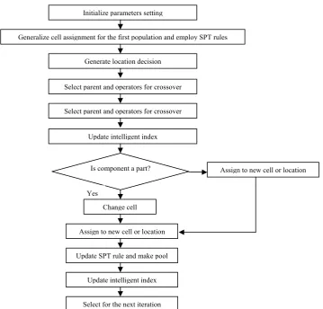
high similarity with the defined matrix in assignment (or with high score) among all parents. Based on above discussions, solution procedure will be performed by the following steps. Step 1) Initialize the necessary parameters used in GA and SA,

Step 2) Generate first population and determine cell formation decision, randomly,

Step 3) Using SPT rule, scheduling decision or the time, generate the first population and assign the machines in different places, randomly,

Step 4) Select parents for crossover operation and generate new solutions based on random combination of parents,

Step 5) Update intelligent index for all existing solutions,

Step 6) Select parents based on intelligent index and perform simulated annealing process and go to step 7, Step 7) If selected component for neighborhood generation set a part go to step 8, otherwise go to step 9, Step 8) Change cell assignment of the part randomly and go to step 10,

Step 9) Select a cell with free capacity and then assign the machine to the new cell and new position or change the location of the machine with another machine located in a same cell. Go to step 10, Step 10) Update SPT method for new solutions achieved by crossover and simulated annealing, Step 11) Determine pool made of parents and new solutions,

Step 12) Update an intelligent index for the next generation, Step 13) Select solutions for the next generation.

Fig. 1. Flowchart of solution procedure

Initialize parameters setting

Generalize cell assignment for the first population and employ SPT rules

Generate location decision

Select parent and operators for crossover

Update intelligent index

Is component a part?

Yes

Change cell

Assign to new cell or location

Update SPT rule and make pool

Update intelligent index

(8)

3.2 Hierarchical solution structure

In order to encode CF and scheduling information for both parts and machines, a two-layer hierarchical schema is proposed. A string of integer numbers in the first layer is applied to encode the CF results for machine and then part genes. In the second layer with s rows, scheduling information

including the time in which operations of each part under each scenario starts and also the location of each machine are indicated. The genes of the first layer are used to control the genes of the second layer in a hierarchical manner. For illustration, consider a data set with 6 parts and 4 machines to be classified into two manufacturing cells under two scenarios. Table 1 shows a typical chromosome structure. The allele of each gene in the first layer represents the cell number in which the machine or part belongs to. For instance, machine 1 is assigned to cell #1 and so on. As such, cell #1 contains machines 1, 2 and 5 and also parts 1, 2, and 4. In the second layer, solution contains two rows representing the time in which operations of each part in a cell under each scenario starts in the left side and also the location of each machine in each cell and under two scenarios on the right side. For example, under scenario 1 and in cell 1, operations part 4 start first and 7 time units later operations of part 3 will start. In addition, Table 1 denotes other information where the difference between sequence starting time in each cell denotes total processing time of prior part. In additions, from table 1, machines M.1 is located in position 1 under scenario 1 and is located in position 2 under scenario 2.

Table 1

Sample of solution structure

P.1 P.2 P.3 P.4 P.5 P.6 M.1 M.2 M.3 M.4

Layer 1: assignment 2 2 1 1 1 2 1 2 2 1

Layer 2: Scheduling & Location 0 11 7 0 15 2 1 2 1 2 _{0 16 0 6 11 8 2 2 1 1}

3.3 Crossover Operator

Selected parents V₁′,V₂′,V₃′,... are grouped to the pairs (V₁′,V₂′),(V₃′,V₄′),.... without loss of generality to

be combined. For all parts and machines, a random real number λ from the open interval (0, 1) is generated. Since each component may be assigned to different cells in each parent, thus in offspring each part or machine must be assigned to one of the cells assigned previously in its parent, randomly with the probability 0.5 based on the value of λ. The crossover operator on V₂′ and V1′ produces one

child X where assignment decisions are illustrated in Fig. 2. Once assignment decisions of new child

have been found, scheduling decisions will be decided by the SPT rule and machines are distributed randomly to the specified locations.

Parent 1 P.1 P.2 P.3 P.4 P.5 P.6 M.1 M.2 M.3 M.4

Parent 2 P.1 P.2 P.3 P.4 P.5 P.6 M.1 M.2 M.3 M.4

Layer 2: Scheduling & Location 8 12 0 0 5 21 2 1 2 1

6 14 0 0 7 25 1 1 2 2

New Solution P.1 P.2 P.3 P.4 P.5 P.6 M.1 M.2 M.3 M.4

(9)

3.4 Simulated annealing features

The main feature of each SA method is to find the best neighborhood solutions where the total solution space can be completely searched. In this section, we describe two approaches in order to find neighborhood solution by SA algorithm. Note that mutation process in GA method is replaced by SA method where decision maker is able to reach the more qualified solutions.

Move type 1: select a part and change the assignment of the selected part to the new cell, randomly Move type 2: select a machine randomly and find the number of the other cells with free capacity so

that the selected machine can be assigned to them. Then, a new cell with free capacity is found randomly and a machine is assigned to the cell.

After each type, since assignment decisions are changed thus all cells must be rescheduled again by SPT rule and location of machines is updated.

4. Numerical Experiments

In order to verify the performance of the hybrid method approach, we have solved 21 random instances. Decision maker has stabilized a time criterion to determine the number of solved instances. In order to generate medium-sized problems, decision maker started from a small-sized problem and increased gently the size of problem by a specific rule (one by one per each parameter) until the exact approach cannot reach the optimum solution within a predetermined running time. In a similar approach, for large-scale problems, decision maker has started from the largest medium-size problem and increase the size of the problem by a specified rule until the branch and bound algorithm cannot find the feasible solution within a predetermined running time. These problems are generated randomly based on the consideration of similar data in the literature. The final numerical results are compared with global solutions obtained by the Lingo 8 software, which uses branch and bound algorithm to solve such problem. We make the following assumption based on the explained discussion.

• A problem is considered small if there is an optimal solution using branch and bound within 5400 seconds.

• A problem is considered medium size whenever branch and bound method can find feasible solution within 5400 seconds.

• A problem is considered large-scale if branch and bound cannot find a feasible solution within 5400 seconds.

• For small-scale problems hybrid method is compared against global solutions and heuristic solutions.

• For medium-scale problems hybrid method is compared against the best solutions by branch and bound algorithm and heuristic solutions.

• For large-scale problems hybrid method is compared against only heuristic solution.

4.1 Effectiveness of hybrid method against branch and bound and heuristic algorithms

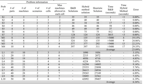
In this section, we present 21 random instances classified into three categories of small, medium and large-scale problems in which they are solve by proposed hybrid method, branch and bound and heuristic procedure introduced in the literature. Table 2 summarizes the details of our computations. For small size problems, it appears that there is not much difference among the entire objective functions obtained by hybrid method algorithm, benchmark heuristic procedure and global optimums. Thus, it is concluded that there is no percentage error when different small-scale problems are selected. It implies that the proposed hybrid genetic algorithm and heuristic procedures are effective to solve the presented model in this class of problems.

(10)

with the best objective function of branch-and-bound method within limited time to measure effectiveness of the introduced hybrid method algorithm. In addition, we have solved these problems by benchmark heuristic procedure to learn more about the behavior of the proposed algorithm. Therefore, the performance evaluation is based on the best objective function found in 5400 seconds using B&B algorithm. These results indicate the comparison among the results obtained by B&B, benchmark algorithm and hybrid method and characteristics of the examples. The last column shows the percentage of gap between B&B and hybrid method solutions. As shown in the last row, the average value of the gap is 23.89%, which indicates better performance of hybrid method compared with the best solutions found by B&B algorithm in limited running time. Indeed, from table 1 when the scale of problems is increased, solutions obtained by benchmark heuristic procedure is located between the solutions of B&B and hybrid method solutions (_Fbound _≤_F*_≤_FBest_{) and therefore, hybrid}

method has a better performance rather than benchmark heuristic algorithm in medium sized problems, too.

For large size problems, we present 10 numerical examples to compare the performance of the proposed hybrid method with the benchmark heuristic solutions. Since Lingo solver cannot obtain feasible solutions for these problems within the maximum running time (5400 seconds), we obtain the best solutions only by benchmark method and it will be a basis to measure performance of the presented hybrid method. In this section, we define a measurement called ‘improvement percent’ computed by (heuristic OFV – hybrid method OFV)/ hybrid method OFV × 100 where OFV is the objective function value. The numerical results reported here and the last row indicates that the average value of improvement percent which is 6.16% implicates to a better performance of hybrid method rather than heuristic procedure for large-scale problems. In other words, hybrid method solutions are better about 6.16% than heuristic solutions, which imply hybrid method is so effective to solve large-scale problems.

Since the proposed method presents better results against heuristic algorithm in almost all examples, therefore the differences between two above methods (i.e. amount of the improvement percent) are strictly significant and the ANOVA test method is not required.

Table 2

Results associated to the numerical experiments

Problem information

Prob

# _parts# of _machines# of _scenarios# of _cells# of

Max machines allowed in

each cell

B&B Solutions

Hybrid method solution

Heuristic Solution

Time B&B (seconds)

Time Hybrid Method (seconds)

Error

S1 4 3 1 3 2 35 35 35 1 <1 0.00%

S2 4 4 1 3 2 40 40 40 1 <1 0.00%

S3 4 3 2 3 2 34 34 34 17 <3 0.00%

S4 5 4 1 3 3 46 46 46 58 <3 0.00%

S5 4 4 2 3 3 49 49 49 37 <3 0.00%

S6 5 4 2 3 3 75 75 75 812 <3 0.00%

S7 7 5 1 3 3 124 124 124 3015 <3 0.00%

M1 8 6 1 3 3 135 135 135 >5400 4 19.15%

M2 9 6 1 3 3 324 324 135 >5400 9 24.86%

M3 9 7 1 3 4 377 377 292 >5400 13 22.21%

M4 10 8 2 3 4 397 397 311 >5400 17 29.35%

Average 23.89%

L1 15 10 2 3 5 - 1090 1056 - - 3.15%

L2 20 13 1 3 6 - 2215 2072 - - 6.45%

L3 30 19 2 4 6 - 4950 4710 - - 4.85%

L4 25 16 2 4 6 - 6224 5876 - - 5.65%

L5 35 22 1 4 6 - 16294 14805 - - 9.14%

L6 40 25 2 4 6 - 25353 23898 - - 5.74%

L7 45 25 1 5 6 - 26615 24936 - - 6.31%

L8 40 28 2 5 7 - 29265 27249 - - 6.89%

L9 50 25 2 6 7 - 35095 32561 - - 7.22%

L10 50 30 2 6 7 - 42092 39487 - - 6.19%

(11)

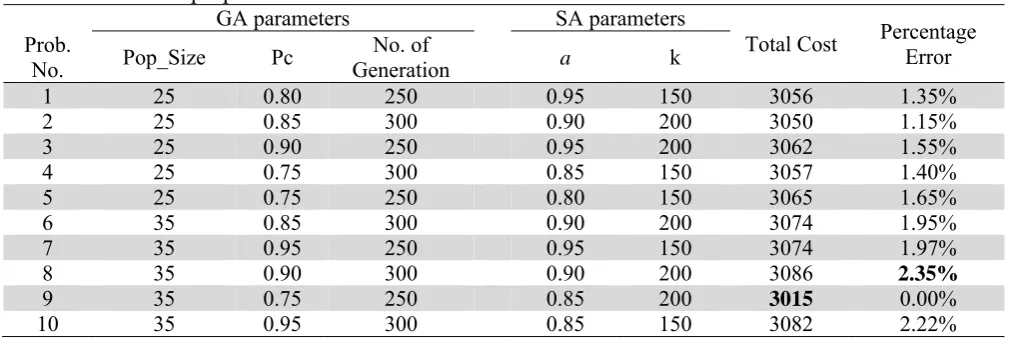
4.2 Robustness of the proposed hybrid method

In Table 3, we compare solutions obtained by hybrid method for problem with 7 parts, 5 machines, 2 scenarios and 4 cells when different parameters in hybrid method approach are taken with the same generations as a stopping rule. It appears that all the minimal costs differ little from each other. From Table 3, the percent error does not exceed 1.65 % when different parameters for hybrid method algorithm are selected, which implies that the hybrid genetic algorithm is robust to the initial parameter settings and effective to solve the model.

Table 3

Robustness of the proposed method

GA parameters SA parameters

Total Cost Percentage Error Prob.

No. Pop_Size Pc Generation No. of a k

1 25 0.80 250 0.95 150 3056 1.35%

2 25 0.85 300 0.90 200 3050 1.15%

3 25 0.90 250 0.95 200 3062 1.55%

4 25 0.75 300 0.85 150 3057 1.40%

5 25 0.75 250 0.80 150 3065 1.65%

6 35 0.85 300 0.90 200 3074 1.95%

7 35 0.95 250 0.95 150 3074 1.97%

8 35 0.90 300 0.90 200 3086 2.35%

9 35 0.75 250 0.85 200 3015 0.00%

10 35 0.95 300 0.85 150 3082 2.22%

5. Conclusions

In this paper, we have introduced a notation of stochastic cell formation problem (SCFP) considering stochastic processing times with discrete scenarios under a supply chain characteristics. A conceptual framework and a novel mathematical formulation were defined. The mathematical method was transformed into a linear model and a hybrid algorithm was introduced to solve the model in large-scale problems. Computational experiments indicated that for large-large-scale problems hybrid method works better than heuristic algorithm. Our contributions research field consists of assuming stochastic parameters which yields more flexibility and practical aspects for real-world cases. It integrates cell formation problem with scheduling and layout aspects under a supply chain and supplier's network, linearization of the model and presenting a hybrid genetic algorithm, which leads to successful performance for any sizes of problem.

Acknowledgment

This research is supported by Grant of Islamic Azad University South Tehran branch by Faculty Research Support Fund from the Faculty of Engineering, Tehran, Iran.

References

Andres, C., Lozano, S., & Adenso-Diaz, B. (2007). Disassembly sequence planning in a Disassembly cell, Robotics and Computer-Integrated Manufacturing, 23(6), 690-695.

Apaioannou, G. P, & Wilson, J. M. (2008). Fuzzy extensions to integer programming of cell formation problem in machine scheduling. Annals of Operations Research, 1-19.

Badiru, A. B. (1992). Computational survey of univariate and multivariate learning curve models,

IEEE Transactions on Engineering Management, 39, 176-188.

Balakrishnan, J., & Cheng C. H., (2005). Dynamic C.M. under multi-period planning horizon,

Journal of Manufacturing Technology Management. 16(5), 516-530.

(12)

Ghosh, T., Sengupta, S., Chattopadhyay, M, & Dan, P. K. (2011). Meta-heuristics in cellular manufacturing: A state-of-the-art review, International Journal of Industrial Engineering Computations, 2, 87-122.

Ghezavati, V. R., & Saidi-Mehrabd, M. (2010). Designing integrated cellular manufacturing systems with scheduling considering stochastic processing time, The International Journal of Advanced Manufacturing Technology, 48 (5-8), 701-717.

Ghezavati, V. R., Jabal-Ameli, M. S., & Makui, A. (2009). A new heuristic method for distribution networks considering service level constraint and coverage radius, Expert Systems with Applications, 36(3), 5620-5629.

Gupta, S.M., & Kavusturucu, A. (1998). Modeling of finite buffer cellular manufacturing systems with unreliable machines. International Journal of Industrial Engineering: Theory Applications and Practice, 5(4), 265-277.

Hurley, S.F., & Whybark, C.D., (1999). Inventory and capacity trade-off in a manufacturing cell.

International Journal of Production Economics Volume, 59(1), 203-212.

Kuroda, M., & Tomita, T., (2005). Robust design of a cellular–line production system with unreliable facilities. Computers and Industrial Engineering, 48(3), 537-551.

Lockwood, W. T., Mahmoodi, F., Ruben, R., Mosier, A., & Charles T. (2000). Scheduling unbalanced cellular manufacturing systems with lot splitting. International Journal of Production Research, 38(4). 951 – 965.

Mahdavi, I., Javadi, B., Fallah-Alipour, K., & Slomp, J. (2007). Designing a new mathematical model for cellular manufacturing system based on cell utilization, Applied Mathematics and Computation, 190, 662–670.

Mobasheri, F., Orren, L. H., & Sioshansi, F. P. (1989). Scenario planning at southern California Edison. INTERFACES, 19(5), 31-44.

Mulvey, J. M. (1996). Generating scenarios for the Towers Perrin investment system. INTERFACES,

26 (2), 1-15.

Shanker, R., & Vrat, P., (1998). Post design modeling for CMS with cost uncertainty, International Journal of Production Economics, 55(1), 97-109.

Shanker, R., & Vrat, P., (1999). Some design issues in C.M. using the fuzzy programming approach.

International Journal of Production Research, 37(11), 2545-2563.

Snyder, L.V. (2006). Facility location under uncertainty: a review, IIE Transactions, 38, 537–554.

Solimanpur, M., Vrat. P., & Shankar, R. (2004). A heuristic to optimize makespan of cell scheduling problem. International Journal of Production Economics, 88, 231–241.

Szwarc, D., Rajamani, D., Bector, C.R, (1997). Cell formation considering fuzzy demand and machine capacity. International Journal of Advanced Manufacturing Technology, 13(2), 134-147.

Tsai, C. C., Chu, C. H., & Barta, T. (1997). Analysis and modeling of a manufacturing cell formation problem with 17. Fuzzy integer programming. IIE Transactions, 29(7), 533–547.

Tavakkoli-Moghaddam, R., Javadian, N., Javadi, B., & Safaei, N. (2007). Design of a facility layout problem in CMS with stochastic demand, Applied Mathematics and Computation, 184(2),

721-728.

Venkataramanaiah, S. (2007). Scheduling in cellular manufacturing systems: an heuristic approach.

International Journal of Production Research, 1, 1-21.