Mining User Contextual Preferences
Sandra de Amo, Marcos L. P. Bueno, Guilherme Alves, Nádia F. Silva
Universidade Federal de Uberlândia, Brazil
[email protected], [email protected], [email protected], [email protected]
Abstract. User preferences play an important role in database query personalization since they can be used for sorting and selecting the objects that most fulfill the user wishes. In most situations user preferences are not static and may vary according to a multitude of user contexts. Automatic tools for extracting contextual preferences without bothering the user are desirable. In this article, we propose CPrefMiner, a mining technique for mining user contextual preferences. We argue that contextual preferences can be naturally expressed by a Bayesian Preference Network (BPN). The method has been evaluated in a series of experiments executed on synthetic and real-world datasets and proved to be efficient to discover user contextual preferences.
Categories and Subject Descriptors: H.Information Systems [H.m. Miscellaneous]: Databases
Keywords: context-awareness, data mining, preference mining
1. INTRODUCTION
Elicitation of Preferences is an area of research that has been attracting a lot of interest within the database and AI communities in recent years. It consists basically in providing the user a way to inform his/her choice on pairs of objects belonging to a database table, with a minimal effort for the user. Preference elicitation can be formalized under either a quantitative [Burges et al. 2005; Crammer and Singer 2001; Joachims 2002] or aqualitative [Jiang et al. 2008; Koriche and Zanuttini 2010; de Amo et al. 2012b; Holland et al. 2003] framework. In order to illustrate the quantitative formulation, consider we are given a collection of movies and we wish to know which films are most preferred by a certain user. For this, we can ask the user to rate each movie and after that we simply select those films with the higher score. This method may be impractical when dealing with a large collection of movies. In order to accomplish the same task using aqualitative formulation of preferences, we can ask the user to inform some generic rules that reflect his/her preferences. For example, if the user says that he/she prefers romance movies to drama movies, then we can infer a class of favorite movies without asking the user to evaluate each film individually.
A qualitative framework for preference elicitation consists in a mathematical model able to express user preferences. In this article, we consider thecontextual preference rules (cp-rules) introduced by [Wilson 2004]. This formalism is suitable for specifying preferences in situations where the choices on the values of an attribute depend on the values of some other attributes (context). For example in our movie database scenario, a user can specify his/her preference concerning the attributegender
depending on the value of the attribute director: For movies whose director isWoody Allen he/she preferscomedy tosuspense and for movies from director Steven Spielberg he/she prefersaction films todrama.
On both frameworks for expressing preferences (quantitative or qualitative), it is important to develop strategies to avoid the inconvenience for the user to report his/her preferences explicitly, a process that can be tedious and take a long time, causing the user not willing to provide such
We thank the Brazilian Research Agencies CNPq, CAPES (SticAmSud Project 016/09) and FAPEMIG for supporting this work.
information. In this context, the development of preference mining techniques allowing the automatic inference of user preferences becomes very relevant.
In this article we propose the algorithm CPrefMiner, a qualitative method for mining a set of
probabilisticcontextual preference rules modeled as apreference bayesian network (BPN). It extends the preliminary version presented in [de Amo et al. 2012a] with the following new features in Section 5: (1) Four new databases have been considered in the tests as well as two different validation protocols; (2) All the experiments have been executed over two baseline algorithms (classical classifiers) in order to show the superiority of CPrefMiner performance as well as the fact that classifiers are not suitable for preference mining tasks; (3) Two parameters aiming at calibrating the user’s indecision and inconsistency have been introduced and a set of experiments have been carried out varying these parameters.
2. RELATED WORK
An extensive text presenting different theoretical approaches and techniques for preference learning can be found in [Fürnkranz and Hüllermeier 2011]. Roughly speaking, preference learning can be divided into two distinct problems: label ranking and object ranking. The problem of Label ranking
consists in discovering rules relating user’s personal information to the way they rank labels. The work of [Hüllermeier et al. 2008] discusses the differences underlying both problems and proposes a method for label ranking consisting in training a set of binary classifiers. On the other hand,object ranking
aims at predicting which is the preferred object between two given objects. The present article focuses on this latter problem.
In [Holland et al. 2003] the authors propose a technique for mining user preferences, based on a qualitative approach, whose underlying model is thepareto preference model. The preference rules are obtained from log data generated by the server when the user is accessing a web site. Another approach to preference mining is presented in [Jiang et al. 2008]. In this work the authors propose using preference samples provided by the user to infer an order on any pair of tuples in the database. Such samples are classified into two categories, thesuperior andinferior samples and contain information about some preferred tuples and some non-preferred ones. From these rules, an order is inferred on the tuples. The underlying preference model is thepareto preference modelas in [Holland et al. 2003]. In this model, preferences are not conditional or contextual, that is, preferences on values of attributes do not depend on the values of other attributes. Our contextual preference model is more expressive.
Concerning the topic of mining contextual preference rules, [Koriche and Zanuttini 2010] proposes a method for mining a CP-Net model [Boutilier et al. 2004] from a set of preferences supplied by the user. Like in our approach, preference samples are represented by ordered pairs of objects. The goal is to identify a target preference ordering with a binary-valued CP-net by interacting with the user through a small number of queries. In [de Amo et al. 2012b] some of the authors of the present article proposed a different method (ProfMiner), based on pattern mining techniques, to discover user
profiles specified by a set of preference rules. The main advantage of CPrefMiner over ProfMiner is that it produces a compact preference model (Bayesian Preference Network), which induces a strict partial order over the set of tuples. Besides, the performance results for both algorithms do not differ significantly, although ProfMiner presents slightly better results than CPrefMiner.
3. PROBLEM FORMALIZATION
Definition 3.1 Preference Database. LetR(A1, A2, ..., An)be a relational schema. Let Tup(R) be the set of all tuples overR. Apreference database overRis a finite setP ⊆Tup(R)×Tup(R) which isconsistent, that is, if(u, v)∈ P then(v, u)6∈ P. The pair(u, v), usually called a bituple, represents the fact that the user prefersthe tuple uto the tuplev.
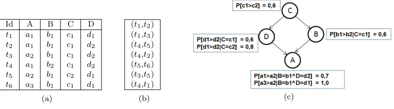
Example 3.2. LetR(A, B, C, D)be a relational schema with attribute domains given by dom(A) ={a1, a2, a3},dom(B) ={b1, b2},dom(C) ={c1, c2}anddom(D) ={d1, d2}. LetIbe an instance overR as shown in Figure 1(a). Figure 1(b) illustrates a preference database overR, representing a sample provided by the user about his/her preferences over tuples ofI.
Id A B C D
t1 a1 b1 c1 d1 t2 a1 b1 c1 d2 t3 a2 b1 c1 d2 t4 a1 b2 c1 d2 t5 a2 b1 c2 d1 t6 a3 b1 c1 d1
(a)
(t1,t2)
(t1,t3)
(t4,t5) (t4,t2) (t5,t6) (t3,t5) (t4,t1)
(b) (c)
Fig. 1: (a) An instanceI, (b) A Preference DatabaseP, (c) Preference NetworkPNet1
The main objective of this article is to extract a contextual preference model from a preference database provided by the user. The contextual preference model is specified by aBayesian Preference Network defined next.
Definition 3.3 Bayesian Preference Network (BPN). ABayesian Preference Network (or BPN for short) over a relational schemaR(A1, ..., An)is a pair (G, θ)where: (1)Gis a directed acyclic graph whose nodes are attributes in {A1, ..., An} and the edges stand for attribute dependency; (2) θ is a mapping that associates to each node of G a conditional probability table of preferences, that is, a finite set of conditional probabilities of the form P[E2|E1] where: (i) E1 is an event of the form
(Ai1 =ai1)∧. . .∧(Aik =aik)such that∀j ∈ {1, ..., k}, aij ∈dom(Aij), and (ii) E2 is an event of
the form “(B =b1) is preferred to (B =b2)”1, whereB is an attribute ofR,B 6=Aij ∀j∈ {1, ..., k} andb1, b2 ∈dom(B),b16=b2.
Example 3.4 BPN. LetR(A, B, C, D)be the relational schema of Example 3.2. Figure 1(c) illus-trates a preference networkPNet1 overR.
Each conditional probabilityP[E2|E1]in a BPN table stands for a probabilisticcontextual prefer-ence rule (cp-rule), where the condition eventE1 is thecontext and the eventE2is thepreference. A probabilistic contextual preference rule associated to a nodeX in the graph Grepresents a degree of belief of preferring some values forX to other ones, depending on the values assumed by its parents in the graph. For instanceP[D =d1> D=d2|C=c1] = 0.6 means that the probability ofD =d1 be preferred toD=d2 is60%given that C=c1.
The quality of a BPN as an ordering tool is measured by means of itsprecision andrecall. In order to properly define the precision and recall of a preference network, we need to define thestrict partial order inferred by the preference network. For lack of space, we do not provide the rigorous definition of the order here, but only describe it by means of an example. For more details see [de Amo and Pereira 2011].
Example 3.5 Preference Order. Let us consider the BPN PNet1 depicted in Figure 1(c). This BPN allows to infer a preference ordering on tuples overR(A, B, C, D). According to this ordering, tuple u1 = (a1, b1,c1,d1) is preferred to tuple u2 = (a2, b2,c1,d2). In order to conclude that, we execute the following steps: (1) Let ∆(u1, u2) be the set of attributes where the u1 and u2 differ. In this example, ∆(u1, u2) = {A, B, D}; (2) Let min(∆(u1, u2)) ⊆ ∆ such that the attributes in min(∆) have no ancestors in∆ (according to graphGunderlying the BPNPNet1). In this example min(∆(u1, u2)) = {D,B}. In order tou1be preferred tou2it is necessary and sufficient thatu1[D]> u2[D] and u1[B] > u2[B]; (3) Compute the following probabilities: p1 = probability that u1 > u2 = P[d1 > d2|C = c1]∗P[b1 > b2|C = c1] = 0.6 * 0.6 = 0.36; p3 = probability that u2 > u1 = P[d2 > d1|C = c1]∗P[b2 > b1|C = c1] = 0.4 * 0.4 = 0.16; p2 = probability that u1 and u2 are incomparable =P[d1 > d2|C =c1]∗P[b2> b1|C =c1] +P[d2 > d1|C =c1]∗P[b1 > b2|C=c1] = 0.6*0.4 + 0.4*0.6 = 0.48. In order to compareu1 and u2 we focus only onp1 and p3 (ignoring the “degree of incomparability” p2) and select the higher one. In this example,p1 > p3 and so, we infer thatu1is preferred tou2. Ifp1=p3we conclude thatu1and u2 are incomparable.
Definition 3.6 Precision and Recall. LetPNetbe a BPN over a relational schemaR. LetP be a preference database overR. The recall of PNet with respect toP is defined by Recall(PNet,P)=
N
M, whereM is the cardinality of P and N is the amount of pairs of tuples (t1, t2)∈ P compatible with the preference ordering inferred byPNeton the tuples t1 andt2. That is, the recall of PNet with respect to P is the percentage of elements in P which are correctly ordered by PNet. The
precision of PNetis defined by Precision(PNet,P)= N
K, whereK is the set of elements ofP which are comparable by PNet. That is, the precision of PNet with respect to P is the percentage of
comparable elements ofP (according toPNet) which are correctly ordered byPNet.
The Mining Problem we treat in this article is the following: Given a training preference database
T1 over a relational schemaRand a testing preference databaseT2overR, find a BPN overRhaving good precision and recall with respect toT2.
4. ALGORITHM CPREFMINER
The task of constructing a Bayesian Network from data has two phases: (1) the construction of a directed acyclic graph G(the network structure) and (2) the computation of a set of parameters θ
representing the conditional probabilities of the model. This work adopts a score-based approach for structure learning.
4.1 Score Function
The main idea of the score function is to assign a real number in[−1,1]for a candidate structureG, aiming to estimate how good it captures the dependencies between attributes in a preference database P. In this sense, each network arc is “punished” or “rewarded”, according to the matching between each arc(X, Y)in Gand the correspondingdegree of dependence of the pair(X, Y)w.r.t. P.
4.1.1 The Degree of Dependence of a Pair of Attributes. The degree of dependence of a pair of attributes(X, Y)with respect to a preference database P is a real number that estimates how pref-erences on values for the attributeY are influenced by values for the attributeX. Its computation is carried out as described in Alg. 1. In order to facilitate the description of Alg. 1 we introduce some notations as follows: (1) For eachy, y′ ∈ dom(Y), y 6=y′ we denote by T
yy′ the subset of bituples (t, t′)∈ P, such thatt[Y] =y∧t′[Y] =y′ ort[Y] =y′∧t′[Y] =y; (2) We define support((y, y′),P) = |Tyy′|
|P| . We say that the pair(y, y′)∈dom (Y)×dom(Y)iscomparable if support((y, y′),P)≥α1, for a given thresholdα1,0≤α1≤1; (3) For each x∈dom(X), we denote bySx|(y,y′)the subset of
Tyy′ containing the bituples (t, t′) such that t[X] =t′[X] =x; (4) We define support(Sx|(y,y′),P) =
|Sx|(y,y′)|
|Sx′ ∈dom(X)Sx′ |(y,y′)|; (5) We say that xis acause for (y, y
′) being comparable if support(S
Algorithm 1:The degree of dependence of a pair of attributes
Input: P: a preference database;(X, Y): a pair of attributes; two thresholdsα1>0andα2>0.
Output: The Degree of Dependence of(X, Y)with respect toP
1 foreach pair(y, y′)∈dom(Y) ×dom(Y), y6=y′ and(y, y′)comparabledo 2 foreachx∈dom(X)wherexis a cause for(y, y′)being comparable do 3 Letf1(S
x|(y,y′)) = max{N,1−N}, where
N =|{(t, t
′)∈S
x|(y,y′):t > t′∧(t[Y] =y∧t′[Y] =y′)}| |Sx|(y,y′)|
4 Letf2(T
yy′) = max{f1(Sx|(y,y′)) :x∈dom(X)} 5 Letf3((X, Y),P) = max{f2(T
yy′) : (y, y
′)∈dom(Y)×dom(Y),y6=y′, (y, y′) comparable}
6 returnf3((X, Y),P)
4.1.2 Score Function Calculus. Given a structureGand a preference databaseP withnattributes,
we definescore(G,P)as score(G,P) =
P
X,Y
g((X, Y), G)
n(n−1) (1)
whereX andY are attributes in a relational schemaR. The functiong is calculated by the following set of rules: (a) Iff3((X, Y), G)≥0.5and edge(X, Y)∈S, theng((X, Y), G) =f3((X, Y), G); (b) If f3((X, Y), G)≥0.5 and edge(X, Y)∈/S, then g((X, Y), G) =−f3((X, Y), G); (c) If f3((X, Y), G)<
0.5and edge(X, Y)∈/S, theng((X, Y), G) = 1; (d) Iff3((X, Y), G)<0.5and edge(X, Y)∈S, then g((X, Y), G) = 0.
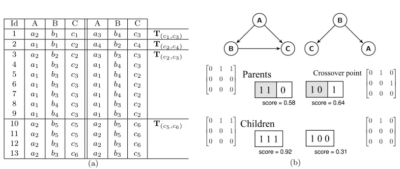
Example 4.1. Let us consider the preference database PrefDb1 = {(t1, t′
2), . . . ,(t13, t′13)}, where t > t′ for every bituple (t, t′) in PrefDb
1 (table at the left side of Figure 2), constructed over a relational schema R(A, B, C), where dom (A) = {a1, . . . , a4}, dom (B) = {b1, . . . , b5} and dom
(C) ={c1, . . . , c6}. In order to compute the degree of dependence of the pair (A, C)with respect to PrefDb1, we first identify the setsTc1,c3 ={(t1, t
′
1)},Tc2,c4={(t2, t
′
2)},Tc2,c3 ={(t3, t
′
3), . . . ,(t9, t′9)} and Tc5,c6 = {(t10, t
′
10), . . . ,(t13, t′13)}. The thresholds we consider are α1 = 0.1 and α2 = 0.2. The support of Tc1,c3, Tc2,c4, Tc2,c3 and Tc5,c6 are 0.08, 0.08, 0.54 and 0.30, respectively. Therefore,
Tc1,c3 and Tc2,c4 are discarded. Entering the inner loop for Tc2,c3 we have only one set S, namely
Sa1|(c2,c3)=Tc2,c3−{(t3, t
′
3)}, sincet3[A]=6 t′3[A]. The support ofSa1|(c2,c3)is6/6 = 1.0andN = 1/6.
Hence,f1(Sa1) = 5/6 andf2(T3) = 5/6. In the same way, forTc5,c6 we haveSa2|(c5,c6)=Tc5,c6 with
support 4/4 = 1.0 and N = 3/4. Therefore, f1(Sa2|(c5,c6)) = 3/4 and f2(T4) = 3/4. Thus, the
degree of dependence of(A, C)is f3((A, C), G) = max{3/4,5/6} = 5/6. The degree of dependence for all pairs, with respect to G, are f3(A, B) = 4/6, f3(B, A) = 0, f3(A, C) = 5/6, f3(C, A) = 0, f3(B, C) = 1, andf3(C, B) = 0.
The score of the networkG1, the left one at Figure 2 (b) is given byscore(G1,PrefDb1) = (4/6 +
1 + 5/6 + 1 + 1 + 1)/6 = 0.92. Let us consider another candidate networkG2, the right one in Figure 2. Its score is given byscore(G2,PrefDb1) = (−4/6 + 0−5/6 + 1 + 1 + 1)/6 = 0.25. By analyzing these values, we conclude that G1 captures more correctly the dependencies between pairs of attributes present in the preference databasePrefDb1than doesG2.
4.2 Mining the BPN Topology
Id A B C A B C
1 a2 b1 c1 a3 b4 c3 T(c1,c3)
2 a1 b1 c2 a4 b2 c4 T(c2,c4)
3 a2 b2 c2 a3 b3 c3 T(c2,c3)
4 a1 b3 c2 a1 b4 c3
5 a1 b3 c3 a1 b4 c2
6 a1 b3 c3 a1 b4 c2
7 a1 b3 c3 a1 b4 c2
8 a1 b4 c3 a1 b3 c2
9 a1 b4 c3 a1 b3 c2
10 a2 b5 c5 a2 b5 c6 T(c5,c6)
11 a2 b5 c5 a2 b5 c6
12 a2 b3 c5 a2 b3 c6
13 a2 b3 c6 a2 b3 c5
(a) (b)
Fig. 2: (a) A preference databasePrefDb1. (b) On top, Bayesian Network StructuresG1 andG2 for the Preference
DatabasePrefDb1. On bottom, crossing over two parents to produce two new individuals. The attribute ordering is ABC. Child with genotype(1,1,1)corresponds to the upper structure shown on top of (b).
4.2.1 Codification of Individuals. To model every possible edge in a Bayesian Network with n
attributes, it is possible to set an×nsquare matrixm, withmij = 1representing the existence of an edge from a nodei to a nodej, and mij = 0otherwise. However, generating random structures and crossing them over in this fashion would potentially create loops. Since a Bayesian Network cannot have loops, this approach would require extra work to deal with this issue.
To avoid this situation, we adopted an upper triangular matrixm, in which every element of the main diagonal and below it are zero. For instance, suppose a database with attributes A,B andC. Considering an orderingABC in m, it is possible forA to be a parent ofB andC. AttributeB can be a parent ofC, but not a parent of A, and so on. This may limit the search abilities of the GA, therefore we doγruns of GA, each one with a different random ordering of attributes, to narrow this issue. In this work, we consideredγ= 50and the number of generations has been settled as 100.
In terms of chromosome genotype, an upper triangular matrix can be implemented as a binary array with n(n2−1) length. An example of this mapping can be seen on the bottom of Figure 2 (b). The initial population contains randomly generated individuals.
4.2.2 Crossover and Mutation Operators. To form a pair of parents to be crossed, initially each one is selected through a mating selection procedure, namely, tournament with size three. It works as follows: randomly select three individuals from the current population, then pick the best of them, i.e., the one with highest score. This procedure is done twice to form each pair of parents, since we need two parents to be crossed. Then, we are ready to apply crossover operator. Since at any generation a given attribute order is fixed, we can use directly two-point crossover to generate two new individuals from two parents. A position from 1 to the length of individual’s size is randomly taken, mixing the genetic materials of two parents, obtaining two new individuals.
The mutation operator aims at adding diversity to population, applying small changes to new individuals, usually under a low probability of occurrence (in this work, 0.05). For each individual generated by crossover, a mutation toggles one position (randomly selected) of its binary array. When an individual is mutated, its score is recalculated, and the mutation is accepted only if it improves its score, otherwise the mutation is discarded.
calculated using Eq. (1). At the end ofj-th generation, we have two populations: parents (Ij) and offspring (I′
j), where|Ij|=|Ij′|=β. In order to attempting to achieve a faster convergence, we use an elitist procedure to select individuals to survive: pick theβ fittest individuals fromIj∪Ij′ to set the next populationIj+1.
4.3 Parameter Estimation
Once we have the topology G of the BPN, calculated at our previous step, we are now seeking for estimates of the conditional probabilities tables. Since we have a set of cases in our prefer-ence databaseP, we can estimate such parameters using the Maximum Likelihood Principle [Jensen and Nielsen 2007], in which we calculate the maximum likelihood estimates for each conditional probability distribution of our model. The underlying intuition of this principle uses frequencies as estimates; for instance, if we want to estimate P(A =a > A=a′|B =b, C =c) we need to calcu-late N(A=a,B=Nb,C(A==ca,B)+N=(b,CA==ac′),B=b,C=c), where N(A=a, B =b, C =c) is the number of cases where (A=a, B=b, C=c)is preferred over(A=a′, B=b, C=c), and so on.
4.4 Complexity Analysis
The optimization problem of determining the Bayesian Network structure which maximizes the score function is intractable. In fact, as shown in [Robinson 1977] the number of possible structures which containsnnodes grows exponentially withn. Thus, heuristic methods having polynomial time com-plexity are normally adopted for accomplishing this task ([Cooper and Dietterich 1992]).
The complexity of creating the model (BPN): (i) the computation of the degree of dependency between each pair of attributes isO(n2.m), wherenis the number of attributes andmis the number of training bituples; (ii) the computation of the topology (carried out by the genetic algorithm (GA)) is O(n2.q.r.γ), where q is the initial population size, r is the number of generations and γ is the number of attribute orderings considered; (iii) the computation of the conditional probability tables isO(e.m), whereeis the number of edges of the BPN produced by the GA. Therefore, the complexity for building the entire CrefMiner model isO(n2(m+q.r.γ)).
The complexity of using the model (BPN) for ordering a bituple (t, t′) is O(n+e), which can be reduced toO(n)when the BPN is a sparse graph. So, one can see that the computational cost for building the model (which is an offline task) is quadratic on the number of attributes n and the computational cost for using the model is linear onn.
5. EXPERIMENTAL RESULTS
In order to devise an evaluation of the proposed methods, in this article we designed experiments over synthetic and real data. A 10-fold cross validation protocol was considered, based on two different sampling strategies. In the following we describe the two sampling strategies, the data features and the results based on each sampling approach.
5.1 The Sampling Strategies for Cross-validation
Let D be a database of tuples of relation schema R(A1, ..., An, Grade), where each tuple over attributes
A1, ..., An has an associated score (grade) given by the user, which specifies his/her preference on this tuple. FromD one can build a preference database P(D)of bituples (u, v) over R(A1, ..., An): (u, v) ∈ P(D)iffu∈D andv∈D, andgrade(u)> grade(v). CPrefMiner is trained and tested over a set of bituples (and not over a set of graded tuples as the classifiers used as baselines in our experiments). Next we describe the two strategies for preparing the training and test data.
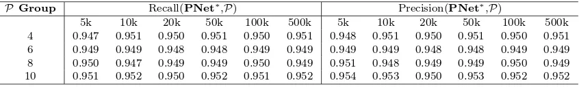
Table I: Preference order assessment, wherePNet∗stands for the best BPN obtained by GA. EachP Groupstands for 9 datasets. The number of attributes is indicated in the first column. The measures appearing in each row correspond to the average measure (recall or precision) between the 9 datasets.
P Group Recall(PNet∗,P) Precision(PNet∗,P)
5k 10k 20k 50k 100k 500k 5k 10k 20k 50k 100k 500k
4 0.947 0.951 0.950 0.951 0.950 0.951 0.948 0.951 0.950 0.951 0.950 0.951 6 0.949 0.949 0.948 0.948 0.949 0.949 0.949 0.949 0.948 0.948 0.949 0.949 8 0.950 0.947 0.949 0.949 0.950 0.949 0.951 0.948 0.949 0.949 0.950 0.949 10 0.951 0.952 0.950 0.952 0.951 0.952 0.954 0.953 0.950 0.953 0.952 0.952
Bti be a subset of Di×Di, where(u, v)∈ Bti iffgrade(u) > grade(v). The tuple-based K -cross-validation protocol executesKrounds of training and testing, where at each round i, the training set isB1∪...∪Bti−1∪Bti+1∪...∪BtK and the testing set isBti. Notice that in this protocol, at each round the bituples involved in the training set do not contain any tuple involved in the testing set.
Bituple-basedK-cross-validation (weak protocol): The preference databaseP(D)is partitioned intoKpairwise disjoint subsets approximately of the same size. The cross-validation in this approach follows the classical protocol, where each round i uses the subset i for testing and the remaining
K−1 subsets of bituples for training. Notice that in this protocol, at each round the testing and training sets are disjoint but individual tuples involved in bituples of the testing set can appear in some training bituple.
5.2 Synthetic Data
Synthetic data2 were generated by an algorithm based on Probabilistic Logic Sampling [Jensen and Nielsen 2007], which samples cases for a preference database P given a BPN with structure Gand parametersθ. We have considered groups of networks with 4, 6, 8 and 10 nodes. For each group, we randomly generated nine networks with their respective parameters. Each attribute at a given setting has a domain with five elements. We also simulated the practical aspect of user’s preference, in the sense that users usually do not elicit their preferences on every pair of objects, so we retained only a small percent (around10−20%) from all possible preference rules that could be generated for a given network structure.
A set of experiments (using the weak protocol for 10-cross-validation) analyzing how a BPN infers the strict partial order described in Sec. 3 is depicted in Table I. We can see that the best BPN obtained by our method returned very good results, both for precision and recall measures. It is possible to note that the small differences between recall and precision, even in cases with large datasets (e.g. 500.000 bituples), indicates that the method leads to very few non-comparable bituples. Apart from that fact, the method infers a correct ordering by a percent around95%in every scenario, having very small data fluctuations, an evidence of the method stability.
5.3 Real Data
In a second series of tests to evaluate CPrefMiner, we considered databases containing preferences re-lated to movies, taken from APMD project3by PRISM Laboratory. Such project integrates data from MovieLens movie recommendation and IMDb forum. Six databases of graded films were considered (films evaluated by six different users), namelyD3,D4,D5,D6,D7andD8. Each database has seven attributes. The experiments have been carried out following the strong and weak 10-cross-validation protocols. The sizes of the setsDi andBti are given in Table II4.
We compare the performance of CPrefMiner with two baselines (the Bayesian classifier and J48), showing the superior quality of the CPrefMiner prediction capability. The poor results produced
2Available athttp://www.lsi.ufu.br/cprefminer/ 3Available at http://apmd.prism.uvsq.fr
Table II: Precision and recall following the weak protocol (bituple-based)
Recall Precision
Dataset Tuples Bituples J48 BayesNet CPrefMiner J48 BayesNet CPrefMiner
D3 167 800 0,173 0,356 0,724 0,506 0,516 0,910
D4 305 2500 0,156 0,432 0,809 0,549 0,613 0,860
D5 607 12000 0,248 0,439 0,864 0,556 0,589 0,887
D6 823 23000 0,270 0,420 0,832 0,487 0,570 0,885
D7 1078 40000 0,345 0,492 0,874 0,556 0,655 0,892
D8 1416 70000 0,295 0,519 0,890 0,596 0,709 0,910
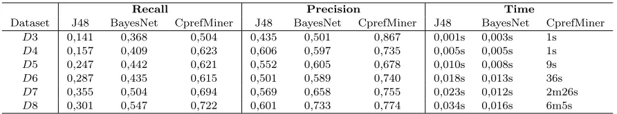
Table III: Precision and recall following the strong protocol (tuple-based)
Recall Precision Time
Dataset J48 BayesNet CprefMiner J48 BayesNet CprefMiner J48 BayesNet CprefMiner
D3 0,141 0,368 0,504 0,435 0,501 0,867 0,001s 0,003s 1s
D4 0,157 0,409 0,623 0,606 0,597 0,735 0,005s 0,005s 1s
D5 0,247 0,442 0,621 0,552 0,605 0,678 0,010s 0,008s 9s
D6 0,287 0,435 0,615 0,501 0,589 0,740 0,018s 0,013s 36s
D7 0,355 0,504 0,694 0,569 0,658 0,755 0,023s 0,012s 2m26s
D8 0,301 0,547 0,722 0,601 0,733 0,774 0,034s 0,016s 6m5s
by these classifiers show that classifiers are not suitable for preference mining tasks. The results concerning the weak protocol are presented in Table II and those concerning the strong protocol in Table III. The execution time forbuilding the BPN is the same for both protocols and is showed only in Table III. In this table we also show the time needed for building the model of the classifiers J48 and BayesNet. The execution times forusing the models are negligible: J48, BayesNet and CPrefMiner take respectively 0.4ms, 1.35ms and 327.53ms for ordering 100 bituples. As expected, the results of precision and recall obtained for CPrefMiner according to the weak protocol are better than those obtained according the strong protocol since for the weak protocol the films appearing in the testing subset may appear in the training set. Remind that a bituple appearing in the test do not appear in the training set. The results show that CPrefMiner, an algorithm specifically designed for a preference mining task, performs far better than classical classifiers.
Parameters for calibrating the inferred order by taking into account the user undecid-ability and inconsistency. Notice that in order to compare two tuples u1 and u2 according to the order described in Example 3.5, we simply ignore the probabilityp2which in some sort measures the user undecidability concerning his/her preferences over these tuples. Notice also that in order to infer a preference we simply consider the higher value between p1 and p3. The proximity of p1 andp3measures in some sort the userinconsistency concerning his/her preferences over these tuples. We could be more precise when defining the preference ordering induced by a BPN by considering parameters k1 and k2 for calibrating respectively the user undecidability and inconsistency factors. That is: we say thatu1is preferred tou2if the following conditions are verified: (1) p2≤k1and (2) p1≥k2(1−p2). The first condition (resp. the second condition) controls how the user undecidability (resp. inconsistency) is taken into account in the inferred ordering. As k1 increases (resp. as k2 decreases) user undecidability (resp. inconsistency) importance decreases for deciding the preference ordering. The ordering considered in Example 3.5 corresponds tok1= 1andk2= 0.5. We designed a set of experiments (over the movie database) intending to evaluate how would be the variation of precision and, specially, recall when we change the values ofk1 and k2 factors. For lack of space we do not present the detailed results. Our conclusion is that the recall decreases very quickly as k1
6. CONCLUSION AND FURTHER WORK
In this article we proposed an approach for specifying contextual preferences using Bayesian Networks and the algorithmCPrefMiner for extracting aBayesian Preference Network from a set of user’s past choices. As future work, we plan to compare the predictive quality of our (optimized) method with well-known ranking methods as RankNet, Rank SVM, Ada Rank and RankBoost [Joachims 2002; Fre-und et al. 2003; Burges et al. 2005; Xu and Li 2007], knowing that existing prototypes that implement these methods have to be adapted (in order to take directly as input pairwise preferences, and not only quantitative preferences). We also intend to deepen the study on the parametersk1 (indecision) and k2 (inconsistency) and design mining techniques which take into account such parameters. Finally, we plan to develop a recommender system using CPrefMiner as a tool for recommending new items for new users without bothering the user with a large amount of sampling evaluations beforehand.
REFERENCES
Boutilier, C.,Brafman, R. I.,Domshlak, C.,Hoos, H. H.,and Poole, D.Cp-nets: A tool for representing and reasoning with conditional ceteris paribus preference statements.Journal of Artificial Intelligence Research.vol. 21, pp. 135–191, 2004.
Burges, C. J. C.,Shaked, T.,Renshaw, E.,Lazier, A.,Deeds, M.,Hamilton, N.,and Hullender, G. N. Learning to Rank Using Gradient Descent. InProceedings of the International Conference on Machine Learning. New York, NY, USA, pp. 89–96, 2005.
Crammer, K. and Singer, Y.Pranking with Ranking. In Proceedings of the Neural Information Processing Systems Conference, Vancouver, Canada, pp. 641–647, 2001.
de Amo, S.,Bueno, M.L.,Alves, G.,Silva, N.F. Mining User Contextual Preferences. InProceedings of the Brazilian Symposium on Databases, São Paulo, Brazil, pp. 177–184 ,2012a.
de Amo, S.,Diallo, M.,Diop, C.,Giacometti, A.,Li, H. D.,and Soulet, A. Mining Contextual Preference Rules for Building User Profiles. InProceedings of the International Conference on Data Warehousing and Knowledge Discovery, Viena, Austria, pp. 229–242, 2012b.
de Amo, S. and Pereira, F.A Context-Aware Preference Query Language: theory and implementation. Tech. Rep., Universidade Federal de Uberlândia, School of Computing, Brazil, 2011.
Cooper, G. F. and Dietterich, T. A Bayesian Method for the Induction of Probabilistic Networks from Data.
Machine Learning,vol. 9(4), pp. 309–347, 1992.
Freund, Y.,Iyer, R.,Schapire, R. E.,and Singer, Y.An efficient boosting algorithm for combining preferences.
Journal of Machine Learning Research,vol. 4, pp. 933–969, 2003.
Fürnkranz, J. and Hüllermeier, E. Preference Learning. Springer, 2011.
Goldberg, D. E.Genetic Algorithms in Search, Optimization & Machine Learning. Addison-Wesley, Massachusetts, 1989.
Holland, S.,Ester, M.,and Kießling, W. Preference Mining: a novel approach on mining user preferences for personalized applications. In European Conference on Principles of Data Mining and Knowledge Discovery, Cavtat-Dubrovnik, Croatia, pp. 204–216, 2003.
Hüllermeier, E.,Fürnkranz, J.,Cheng, W.,and Brinker, K.Label Ranking by Learning Pairwise Preferences.
Artificial Intelligence,vol. 172(16-17), pp. 1897–1916, 2008.
Jensen, F. V. and Nielsen, T. D. Bayesian Networks and Decision Graphs. Springer Publ. Company, Inc., 2007. Jiang, B.,Pei, J.,Lin, X.,Cheung, D. W.,and Han, J.Mining Preferences from Superior and Inferior Examples.
In ACM SIGKDD Conference on Knowledge Discovery and Data Mining, Las Vegas, Nevada, USA, pp. 390–398, 2008.
Joachims, T. Optimizing Search Engines using Clickthrough Data. In Proceedings of the 8th ACM SIGKDD Inter-national Conference on Knowledge Discovery and Data Mining, Edmonton, Alberta, Canada, pp. 133–142, 2002. Koriche, F. and Zanuttini, B. Learning Conditional Preference Networks. Artificial Intelligence,vol. 174(11), pp.
685–703, 2010.
Robinson, R. W.Counting Unlabeled Acyclic Digraphs. In C.H.C. Little (Ed.)Combinatorial Mathematics. Lecture Notes in Mathematics, vol. 622. New York, Springer-Verlag, 1977.
Wilson, N.Extending CP-Nets with Stronger Conditional Preference Statements. InNational Conference on Artificial Intelligence, San Jose, California, USA, pp. 735–741, 2004.