P R O C E E D I N G S
Open Access
Decomposing PPI networks for complex
discovery
Guimei Liu
1*, Chern Han Yong
2, Hon Nian Chua
3, Limsoon Wong
1From
International Workshop on Computational Proteomics
Hong Kong, China. 18-21 December 2010
Abstract
Background:Protein complexes are important for understanding principles of cellular organization and functions. With the availability of large amounts of high-throughput protein-protein interactions (PPI), many algorithms have been proposed to discover protein complexes from PPI networks. However, existing algorithms generally do not take into consideration the fact that not all the interactions in a PPI network take place at the same time. As a result, predicted complexes often contain many spuriously included proteins, precluding them from matching true complexes.
Results:We propose two methods to tackle this problem: (1) The localization GO term decomposition method: We utilize cellular component Gene Ontology (GO) terms to decompose PPI networks into several smaller networks such that the proteins in each decomposed network are annotated with the same cellular component GO term. (2) The hub removal method: This method is based on the observation that hub proteins are more likely to fuse clusters that correspond to different complexes. To avoid this, we remove hub proteins from PPI networks, and then apply a complex discovery algorithm on the remaining PPI network. The removed hub proteins are added back to the generated clusters afterwards. We tested the two methods on the yeast PPI network
downloaded from BioGRID. Our results show that these methods can improve the performance of several complex discovery algorithms significantly. Further improvement in performance is achieved when we apply them in tandem.
Conclusions:The performance of complex discovery algorithms is hindered by the fact that not all the
interactions in a PPI network take place at the same time. We tackle this problem by using localization GO terms or hubs to decompose a PPI network before complex discovery, which achieves considerable improvement.
Introduction
High-throughput experimental techniques have pro-duced large amounts of protein interactions, which makes it possible to discover protein complexes from protein-protein interaction (PPI) networks. A PPI net-work can be modeled as an undirected graph, where vertices represent proteins and edges represent interac-tions between proteins. Protein complexes are groups of proteins that interact with one another, so they are usually dense subgraphs in PPI networks. Many
algorithms have been developed to discover complexes from PPI networks [1-8].
As a model organism, Saccharomyces cerevisiae
(baker’s yeast) has been extensively studied, and its PPI network is now relatively complete. However, the per-formance of existing complex discovery algorithms on the yeast PPI network is not very satisfactory. One rea-son behind this is that each protein do not necessarily participate in all its known interactions simultaneously. With very few exceptions [9], existing complex discovery algorithms generally do not take this into consideration. As a result, the clusters generated often contain extra proteins that preclude them from matching true com-plexes. An ideal solution would be to decompose the * Correspondence: [email protected]
1School of Computing, National University of Singapore, Singapore
Full list of author information is available at the end of the article
PPI network into several smaller networks such that interactions within each smaller network are contex-tually coherent. In reality, it is very difficult to know which subset of interactions take place together. Here we choose to use cellular component GO terms to decompose PPI networks because a protein complex can be formed only if its proteins are localized within the same compartment of the cell. We use only localization GO terms that are relatively general for decomposition. The existence of hub proteins is another factor that makes it difficult for complex discovery algorithms to decide the boundary of clusters. Hub proteins are pro-teins that have a lot of neighbors in the PPI network, and these neighbors often belong to multiple complexes [10]. This may fuse clusters that correspond to different complexes. To avoid this, we remove hub proteins from PPI networks prior to clustering. After the clusters are generated from the remaining PPI network, we then add the removed hub proteins back to the clusters.
We tested the above methods on the yeast PPI net-work downloaded from BioGRID [11]. The results show that these methods can improve the performance of existing complex discovery algorithms significantly. A preliminary version of this paper was presented as a short paper [12] in BIBM2010. In this version, we have included more experimental results and further dis-cussed why some complexes are so hard to detect. In the rest of the paper, we first describe the two methods for decomposing PPI networks, and then show experi-ment results.
Methods
In this section, we first describe the two methods for decomposing PPI networks for complex discovery, and then briefly introduce the complex discovery algorithms used in our experiments.
The localization GO term decomposition method
A protein complex can only be formed if its proteins are localized within the same compartment of the cell. Hence we use cellular component GO terms to decom-pose a given PPI network into several smaller PPI net-works such that all proteins in each smaller network are annotated with the same localization GO term. We use only localization GO terms that are relatively general for decomposition. There are several reasons for this. First, it is relatively easy to obtain the rough localization of proteins, compared with obtaining the precise and speci-fic localization of proteins. Secondly, very specispeci-fic GO terms are annotated to very few proteins. Using them to decompose PPI networks produces many small frag-ments, and lots of information may be lost due to the
decomposition. Finally, some very specific cellular com-ponent GO terms correspond to complexes, and they are just as hard to decide as complexes.
We use a threshold NGO to select GO terms for
decomposition, whereNGOshould be large. The selected GO terms are annotated to at least NGO proteins, and none of their descendant terms is annotated to at least NGOproteins. If a GO term is selected, then none of its ancestor terms or descendant terms will be selected.
Given a selected GO term, we first remove all the pro-teins that are not annotated to the term from the given PPI network, and then apply a complex discovery algo-rithm on the resultant network. This process is repeated for every selected GO term. The final set of clusters is the union of the clusters discovered from every filtered network. Duplicated clusters are removed.
The hub removal method
Hub proteins are those proteins that have many neigh-bors in the PPI network. We use a threshold Nhub to define hub proteins. We call a protein ahub proteinif it has at leastNhub neighbors. A hub protein often con-nects proteins that belong to different complexes, which makes it hard to decide the boundary of the complexes and the membership of the hub proteins.
To alleviate the impact of the hub proteins, we first remove hub proteins from a given PPI network, and then use an existing complex discovery algorithm to find clusters from the remaining network. After the clusters are generated, hub proteins are added back to the clusters. We add a hub proteinuback to a clusterC based on the connectivity between u and C, which is defined as follows:
Connectivity u C
w u v
C
v C ( , )
( , )
=
∑
∈ (1)where w(u,v) is the weight of edge (u,v), and it is cal-culated from the original PPI network using iterative AdjustCD [8] before removing hubs. If there is no edge between u andv, then w(u, v)=0. A hub protein u is added to a cluster C only if Connectivity(u, C) ≥
hub_add_thres, where hub_add_thres is a number
between 0 and 1.
Combining the two methods
We combine the two methods by first removing hub proteins from the given PPI network, and then decom-posing the resultant PPI network using selected GO terms. The whole process is described below:
2. Remove hub proteins that have at leastNhub neigh-bors from the given PPI networkG. LetG′be the resul-tant network.
3. Letg1,...,gm be the localization GO terms that are selected using threshold NGO. For each gi, do the following:
•Remove proteins that are not annotated withgifrom G′. Let G′i be the resultant network.
•Apply a complex discovery algorithm on G′i to find clusters. Let i be the set of clusters generated.
• = i;
4. Remove duplicated clusters from . 5. Add hub proteins back to clusters in .
Complex discovery algorithms
We used the following complex discovery algorithms in our study. MCL and RNSC generate a partition of the PPI network, and they do not allow overlap among clus-ters. The other two algorithms, IPCA and CMC, allow overlap among clusters.
Markov Cluster Algorithm (MCL) [1] is motivated by a heuristic formulated in terms of stochastic flow. It iteratively enhances the contrast between regions of strong and weak flow in the graph. The process con-verges towards a partition of the graph, with a set of high-flow regions (the clusters) separated by boundaries with no flow. The performance of MCL is mainly affected by the“-I inflation” option, which controls the granularity of the output clustering.
Restricted Neighborhood Search Clustering (RNSC) [13] is a cost-based local search algorithm that explores the solution space to minimize a cost function, calcu-lated according to the number of intra-cluster and inter-cluster edges. RNSC searches for a low-cost inter-clustering by first composing an initial random clustering, and then iteratively moving a node from one cluster to another in a randomized fashion to reduce the cluster-ing’s cost. It also makes diversification moves to avoid local minima. RNSC performs several runs, and reports the clustering from the best run. The number of runs is controlled by the“-e” option.
IPCA[7] follows the general approach of cluster
expanding based on seeded vertices. It first assigns weights to edges and vertices, and then picks the vertex with the highest weight as the seed of a new cluster. Other vertices are then added to the cluster based on their connectivity. For each of the subsequent cluster, the vertex with the highest weight among those vertices that do not appear in previous clusters is chosen as the seed, and the cluster is expanded using all the vertices except those seed vertices in the previous clusters. Whether a vertex can be added to a cluster is deter-mined by the diameter of the resultant cluster (the“-P”
option) and the connectivity between the vertex and the cluster (the “-T”option).
Clustering by Maximal Cliques (CMC) [8] first gener-ates all the maximal cliques from a given PPI network, and then removes or merges highly overlapping cliques based on their inter-connectivity as follows. Each maxi-mal clique is assigned a score based on their weighted density and size. If the overlap between two maximal cliques exceeds a threshold overlap_thres, then CMC checks whether the inter-connectivity between the two cliques exceeds a thresholdmerge_thres. If it does, then the two cliques are merged together; otherwise, the cli-que with lower score is removed.
Results and discussion
In this section, we first describe the datasets and the eva-luation method used in our experiments, and then study the impact of the two decomposition methods on the performance of the four complex discovery algorithms.
Experiment settings
PPI data
We used the yeast PPI dataset downloaded from Bio-GRID [11] (version 3.0.64) in our experiments. We kept only physical interactions that are generated by the fol-lowing experiment types:Affinity Capture-Luminescence,
Affinity Capture-MS, Affinity Capture-RNA, Affinity
Capture-Western,Biochemical Activity,Co-crystal Struc-ture,Co-fractionation, Co-localization,Co-purification, Far Western,FRET,PCA,Protein-peptide,Protein-RNA, Reconstituted Complex, Two-hybrid. Self-interactions are removed. The dataset contains 5765 proteins and 52096 binary interactions.
Evaluation methods
We match the generated clusters with reference com-plex sets, and calculate recall (sensitivity) and precision. LetSbe a cluster, Cbe a reference complex, VSandVC be the set of proteins contained inSandCrespectively. We define the matching score between Sand Cas the Jaccard index betweenVS andVC.
match score S C V V
V V
S C S C
_ ( , )=
(2)
Given a thresholdmatch_thres, ifmatch_score(S,C)≥
match_thres, then we say S and C match each other.
Given a set of reference complexes ={C C1, 2,,Cn} and a set of predicted complexes ={ ,S S1 2,,Sm}, recall and precision are defined as follows:
Recall
C Ci i Sj S matches Cj i
=
{
∈ ∧ ∃ ∈ }
,
Precision
S Sj j Ci C matches Si j
=
{
∈ ∧ ∃ ∈,}
(4)There is often an inverse relationship between preci-sion and recall. We combine the two measures into a single measure called F1-measure to assess the overall performance. F1-measure is defined as follows:
F ecision
ecision
1= ⋅2 ⋅
+
Pr Recall
Pr Recall (5)
Reference complexes
Three reference sets of protein complexes are used in our experiments. Two set of complexes are hand-curated complexes from MIPS [14] and the CYC2008 catalogue [15]. The third set is generated by Aloy et al. [16]. We combine these three sets of complexes together, and keep only those complexes with size no less than 4. Duplicated complexes are removed. Table 1 shows the number of complexes, number of proteins, the maximal, average and median size, and the average and median density of the complexes in the three refer-ence complex sets and the combined set. In all the experiments below, we used the combined reference complex set, and considered complexes and clusters with size no less than 4.
Parameter settings of the four complex discovery algorithms
Unless stated explicitly, the parameters of the four com-plex discovery algorithms are set as in Table 2. Para-meters not shown are set to their default values.
Results of the GO term decomposition method
The first experiment studies the impact of the GO term decomposition method on the performance of the four
algorithms. We use annotations in Gene Ontology [17] (dated 4 June, 2010) to select GO terms for decomposi-tion. Table 3 shows the number of GO terms selected under differentNGOvalues. If a protein is annotated to none of the selected GO terms, then the protein is dis-carded because it does not occur in any of the small PPI networks after decomposition. The number of such pro-teins is shown in the third column. If the two propro-teins of an interaction do not share a common selected GO term, then the two proteins do not occur in any com-mon PPI network after decomposition and the interac-tion between them is lost too. The number of such interactions is shown in the last column of Table 3. The number of proteins and interactions that are discarded is considerably large whenNGOis small.
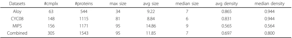
Figures 1 shows the recall and precision of the four complex discovery algorithms when differentNGO thresh-olds are used for selecting localization GO terms. The pre-cision of all the four algorithms is improved considerably under all the differentNGOvalues. The recall is improved as well whenNGO≥300. WhenNGO=30 or 100, recall of the four algorithms decreases. This is mainly because too much information is lost in these two cases as shown in Table 3. Hence we should use GO terms that are relatively general to decompose PPI networks to avoid breaking the whole network into tiny fragments. Overall, the perfor-mance of all the four algorithms improves. We have also tested other parameter settings of the four complex dis-covery algorithms besides that shown in Table 2. The improvements achieved are all very similar.
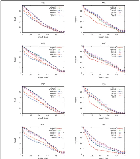
We also compared the above improvement with that of using random protein groups for decomposition. Ran-dom protein groups are generated by replacing proteins of the selected GO terms with randomly picked proteins. We generated 100 sets of random protein groups and use their mean F1-measure as the result. Figures 2 shows
Table 1 Statistics of reference complexes
Datasets #cmplx #proteins max size avg size median size avg density median density
Aloy 63 544 34 9.22 7 0.865 0.944
CYC08 148 1115 81 8.84 6 0.831 0.944
MIPS 156 1171 95 14.86 9 0.565 0.564
Combined 305 1543 95 11.85 7 0.697 0.800
Only complexes of size≥4 are considered.
Table 2 Parameter settings of complex discovery algorithms
algorithms parameter settings
MCL -I 1.8
RNSC -e10 -D50 -d10 -t20 -T3 IPCA -T0.4
CMC overlap_thres=0.5,merge_thres=0.4
Table 3 Number of GO terms selected under different
NGOvalues
NGO #GO terms selected #proteins discarded #PPIs discarded
1000 6 2067 27151
500 10 2193 27477
300 10 2481 33425
100 29 3023 39992
0 0.2 0.4 0.6 0.8 1
0 0.2 0.4 0.6 0.8 1
Recall
match_thres MCL
original GO1000 GO500 GO300 GO100 GO30
0 0.2 0.4 0.6 0.8 1
0 0.2 0.4 0.6 0.8 1
Precision
match_thres MCL
original GO1000 GO500 GO300 GO100 GO30
0 0.2 0.4 0.6 0.8 1
0 0.2 0.4 0.6 0.8 1
Recall
match_thres RNSC
original GO1000 GO500 GO300 GO100 GO30
0 0.2 0.4 0.6 0.8 1
0 0.2 0.4 0.6 0.8 1
Precision
match_thres RNSC
original GO1000 GO500 GO300 GO100 GO30
0 0.2 0.4 0.6 0.8 1
0 0.2 0.4 0.6 0.8 1
Recall
match_thres IPCA
original GO1000 GO500 GO300 GO100 GO30
0 0.2 0.4 0.6 0.8 1
0 0.2 0.4 0.6 0.8 1
Precision
match_thres IPCA
original GO1000 GO500 GO300 GO100 GO30
0 0.2 0.4 0.6 0.8 1
0 0.2 0.4 0.6 0.8 1
Recall
match_thres CMC
original GO1000 GO500 GO300 GO100 GO30
0 0.2 0.4 0.6 0.8 1
0 0.2 0.4 0.6 0.8 1
Precision
match_thres CMC
original GO1000 GO500 GO300 GO100 GO30
that using random protein groups to decompose the PPI network decrease the performance of the four algorithms greatly, where the random protein groups were generated from GO terms selected at a threshold of 500.
Results of the hub removal method
The second experiment studies the impact of the hub removal method on the performance of the four algo-rithms. Table 4 shows the number of hub proteins and interactions removed under differentNhub values. The numbers indicate that a small number of hub proteins account for a large number of interactions. For example, the percentage of proteins with at least 100 neighbors is less than 2%, while they account for about 37% of the interactions.
We use parameterhub_add_thresto determine when
a hub can be added to a cluster. In our experiments, we found that the proper range forhub_add_thres is [0.2, 0.9]. In the rest of the experiments, we set hub_add_thresto 0.3.
0 0.2 0.4 0.6 0.8 1
0 0.2 0.4 0.6 0.8 1
F1
match_thres MCL
original GO500 Random Protein Groups
0 0.2 0.4 0.6 0.8 1
0 0.2 0.4 0.6 0.8 1
F1
match_thres RNSC
original GO500 Random Protein Groups
0 0.2 0.4 0.6 0.8 1
0 0.2 0.4 0.6 0.8 1
F1
match_thres IPCA
original GO500 Random Protein Groups
0 0.2 0.4 0.6 0.8 1
0 0.2 0.4 0.6 0.8 1
F1
match_thres CMC
original GO500 Random Protein Groups
(a) MCL (b) RNSC
(c) IPCA (d) CMC
Figure 2F1-measure of the four algorithms when random protein groups are used for decomposition
Table 4 #hub proteins and #PPIs removed under differentNhub
Nhub #hub proteins removed #PPIs removed
100 97 19292
75 207 26331
50 446 35632
40 651 40534
30 996 45568
0 0.2 0.4 0.6 0.8 1
0 0.2 0.4 0.6 0.8 1
Recall
match_thres MCL
original h=100 h=75 h=50 h=40 h=30 h=20
0 0.2 0.4 0.6 0.8 1
0 0.2 0.4 0.6 0.8 1
Precision
match_thres MCL
original h=100 h=75 h=50 h=40 h=30 h=20
0 0.2 0.4 0.6 0.8 1
0 0.2 0.4 0.6 0.8 1
Recall
match_thres RNSC
original h=100 h=75 h=50 h=40 h=30 h=20
0 0.2 0.4 0.6 0.8 1
0 0.2 0.4 0.6 0.8 1
Precision
match_thres RNSC
original h=100 h=75 h=50 h=40 h=30 h=20
0 0.2 0.4 0.6 0.8 1
0 0.2 0.4 0.6 0.8 1
Recall
match_thres IPCA
original h=100 h=75 h=50 h=40 h=30 h=20
0 0.2 0.4 0.6 0.8 1
0 0.2 0.4 0.6 0.8 1
Precision
match_thres IPCA
original h=100 h=75 h=50 h=40 h=30 h=20
0 0.2 0.4 0.6 0.8 1
0 0.2 0.4 0.6 0.8 1
Recall
match_thres CMC
original h=100 h=75 h=50 h=40 h=30 h=20
0 0.2 0.4 0.6 0.8 1
0 0.2 0.4 0.6 0.8 1
Precision
match_thres CMC
original h=100 h=75 h=50 h=40 h=30 h=20
Figure 3Recall and precision of the four algorithms when differentNhubvalues are used for removing hubsThe X-axis ismatch_thres.
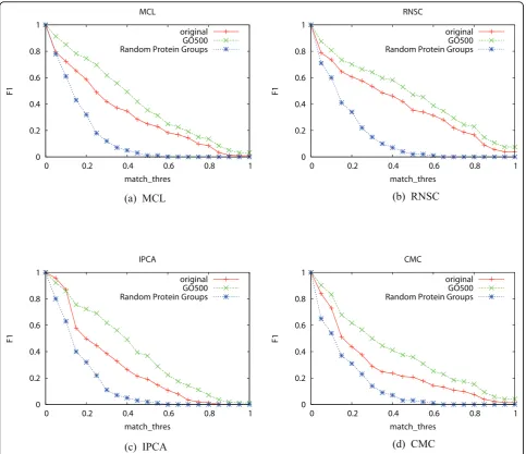
Figures 3 shows the recall and precision of the four
complex discovery algorithms when different Nhub
thresholds are used for removing hub proteins. The recall of the four algorithms decreases greatly when Nhub≤ 30, which indicates that too many proteins and interactions are removed as shown in Table 4. The hub removal strategy is not helpful for RNSC and MCL, but is very helpful for IPCA and CMC. The main improve-ment of IPCA and CMC is on precision.
It has been proposed that two types of hubs exist: party hubs that interact with all their neighbours simul-taneously, and date hubs that interact with different neighbours at different times [10]. We postulate that whenNhub≥ 30, most of the hubs removed correspond
to date hubs, as it is physically unlikely for a protein to bind to so many other proteins at the same time due to its limited surface area. However, when removing hubs with fewer neighbours, it might be helpful to identify and remove only date hubs, while ignoring party hubs.
0 0.2 0.4 0.6 0.8 1
0 0.2 0.4 0.6 0.8 1
F1
match_thres MCL
original GO500 Hub50 Hub50+GO500
0 0.2 0.4 0.6 0.8 1
0 0.2 0.4 0.6 0.8 1
F1
match_thres RNSC
original GO500 Hub50 Hub50+GO500
0 0.2 0.4 0.6 0.8 1
0 0.2 0.4 0.6 0.8 1
F1
match_thres IPCA
original GO500 Hub50 Hub50+GO500
0 0.2 0.4 0.6 0.8 1
0 0.2 0.4 0.6 0.8 1
F1
match_thres CMC
original GO500 Hub50 Hub50+GO500
(a) MCL (b) RNSC
(c) IPCA (d) CMC
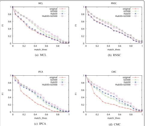
Figure 4F1-measure of the four algorithms when the two methods are performed in tandemThe X-axis ismatch_thres.“original”means the original network with neither hub removal nor GO term decomposition.“GO500”means that the network is decomposed using GO terms selected at a threshold of 500.“Hub50”means that hub proteins with at least 50 neighbors are removed.“Hub50+GO500”means that first hub proteins with at least 50 neighbors are removed, and the network is then decomposed using GO terms selected at a threshold of 500.
Table 5 F1-measure of the four algorithms when
match_thres=0.5
original Hub50 GO500 Hub50+GO500
MCL 0.250 0.272 0.354 0.406
RNSC 0.353 0.347 0.471 0.436
IPCA 0.191 0.405 0.368 0.469
To test this hypothesis, we removed only hubs that are part of at least 3, 5, or 7 reference complexes, forNhub =5-9, 10-14, or 15-19. This experiment assumes that we have a classifier which is able to accurately distinguish between date hubs (hubs that belong to many reference complexes) and party hubs (hubs that belong to fewer complexes). However, none of these settings show any significant improvement over not removing these hubs with fewer neighbours, possibly because too few hubs were removed to have a significant impact on performance.
Results of combining the two methods
The last experiment is to examine the combined impact of the two decomposition methods. We set NGO to 500 andNhubto 50. Figures 4 shows the results. RNSC and MCL do not benefit much from the hub removal method, so for these two algorithms, combining the two decomposition methods yields little improvement com-pared with using GO decomposition alone. The perfor-mance of IPCA and CMC improve when both methods are used.
Table 5 shows the F1 of the four algorithms when
match_thres=0.50. RNSC shows the best performance
on the original PPI network, while CMC performs the best when the two decomposition methods are used.
Discussion
Even though the performance of the four algorithms improves significantly after applying the two
pre-processing methods, many reference complexes remains undetected by all four algorithms. On the original net-work, 116 reference complexes cannot be detected by any of the four complex discovery algorithms when
match_thres=0.5. This number reduces slightly to 113
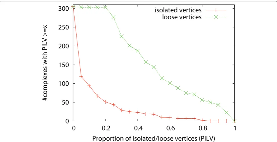
after applying the two pre-processing methods. To find out why these complexes cannot be detected, we study the density of the reference complexes and the connec-tivity of the vertices in the complexes. We define a ver-tex in a complex as an isolated vertexif it connects to none of the other vertices in the same complex. We define a vertex in a complex as a loose vertex if it con-nects to less than half of the other vertices in the same complex. Complexes with low density or containing many isolated/loose vertices are very difficult to detect. Figure 5 shows the density of the complexes. Figure 6 shows the proportion of isolated vertices and loose ver-tices in the complexes. Among the 305 complexes, 81 complexes have a density less than 0.5, and 42 plexes have a density less than 0.25. There are 144 com-plexes with more than half of their proteins being loose proteins, and these complexes are not easy to detect. There are 18 complexes with more than half of their proteins being isolated vertices, and these complexes are almost impossible to discover. Figure 7 shows the den-sity of the complexes that are detected or are not detected separately. Most of the complexes that are detected have high density. For all the four algorithms, 90% of the detected complexes have a density no less than 0.5. On the contrary, many complexes that are not
0
50
100
150
200
250
300
0
0.2
0.4
0.6
0.8
1
#complexes with density >=x
Density
detected have a density less than 0.5, and they also have many loose vertices. There are some complexes that have very high density but cannot be discovered by the four algorithms. We found that for such complexes, usually there exists some cluster such that the complex is a subset of the cluster but the size of the cluster is too large to qualify as a match. If we lower the matching threshold to 0.33, then most of these high density com-plexes can be matched by some clusters.
Conclusions
In this paper, we proposed two methods to decompose PPI networks for complex discovery. We used four com-plex discovery algorithms to experimentally study the effectiveness of the two methods. The results show that the two decomposition methods help improve the per-formance of the four algorithms significantly. The two partitioning clustering algorithms, MCL and RNSC, ben-efit more from the GO decomposition method, while
0
50
100
150
200
250
300
0
0.2
0.4
0.6
0.8
1
#complexes with PILV >=x
Proportion of isolated/loose vertices (PILV)
isolated vertices
loose vertices
Figure 6Distribution of isolated/loose vertices in complexesThe X-axis is the proportion of isolated/loose vertices in a complex. The Y-axis is the number of complexes with proportion of isolated/loose vertices >=x.
0 50 100 150 200
0 0.2 0.4 0.6 0.8 1
#matched complexes with density >=x
Density
MCL RNSC IPCA CMC
0 20 40 60 80 100 120 140 160 180
0 0.2 0.4 0.6 0.8 1
#unmatched complexes with density >=x
Density
MCL RNSC IPCA CMC
(a) matched reference complexes (b) unmatched reference complexes
the two algorithms that allow overlap among clusters, CMC and IPCA, benefit from both.
For the GO term decomposition method, we recom-mend using localization GO terms that are relative gen-eral because their annotations are easier to obtain and they also preserve more information than GO terms that are very specific.
There are two main reasons why some complexes can-not be detected. First, there might be too few interac-tions existing between proteins in the complex. Secondly, the complex itself might be densely con-nected, but so is the region surrounding it, which makes it difficult to correctly delineate the boundary around it. Both cases are difficult to handle. We may need to use other information besides PPI data to detect such complexes.
Acknowledgements
This work was supported in part by a Singapore National Research Foundation grant NRF-G-CRP-2007-04-082(d) (Wong, Liu) and by a National University of Singapore NGS scholarship (Yong).
This article has been published as part ofProteome ScienceVolume 9 Supplement 1, 2011: Proceedings of the International Workshop on Computational Proteomics. The full contents of the supplement are available online at http://www.proteomesci.com/supplements/9/S1.
Author details 1
School of Computing, National University of Singapore, Singapore.2NUS Graduate School for Integrative Sciences and Engineering, National University of Singapore, Singapore.3Data Mining Department, Institute for
Infocomm Research, Singapore.
Authors’contributions
GL conducted the experiments and wrote this manuscript. CHY and HNC gave suggestions on the proposed methods as well as the performance study. They also helped improve the manuscript. LW guided the study and improved the writing of the manuscript. All authors read and approved the final manuscript.
Competing interests
The authors declare that they have no competing interests.
Published: 14 October 2011
References
1. van Dongen S:Graph clustering by flow simulation.PhD thesis, University of Utrecht2000.
2. Przulj N, Wigle D:Functional topology in a network of protein interactions.Bioinformatics2003,20(3):340-348.
3. Bader G, Hogue C:An automated method for finding molecular complexes in large protein interaction networks.BMC Bioinformatics2003, 4(2).
4. Altaf-Ul-Amin M, Shinbo Y, Mihara K, Kurokawa K, Kanaya S:Development and implementation of an algorithm for detection of protein complexes in large interaction networks.BMC Bioinformatics2006,7(207).
5. Adamcsek B, Palla G, Farkas I, Derenyi I, Vicsek T:CFinder:locating cliques and overlapping modules in biological networks.Bioinformatics2006, 22(8):1021-1023.
6. Chua H, Ning K, Sung W, Leong H, Wong L:Using indirect protein-protein interactions for protein complex predication.Journal of Bioinformatics and Computational Biology2008,6(3):435-466.
7. Li M, Chen J, Wang J, Hu B, Chen G:Modifying the DPClus algorithm for identifying protein complexes based on new topological structures.BMC Bioinformatics2008,9(398).
8. Liu G, Wong L, Chua HN:Complex discovery from weighted PPI networks.Bioinformatics2009,25(15):1891-1897.
9. Habibi M, Eslahchi C, Wong L:Protein Complex Prediction based on k-Connected Subgraphs in Protein Interaction Network.BMC Systems Biology2010,4:129.
10. Han JDJ, Bertin N, Hao T, Goldberg DS, Berriz GF, Zhang LV, Dupuy D, Walhout AJM, Cusick ME, Roth FP, Vidal M:Evidence for dynamically organized modularity in the yeast protein-protein interaction network. Nature2004,430:88-93.
11. Stark C, Reguly BJBT, Boucher1 L, Breitkreutz1 A, Tyers M:BioGRID: a general repository for interaction datasets.Nucleic Acids Research2006, 34(Database Issue):535-539.
12. Liu G, Yong CH, Chua HN, Wong L:Decomposing PPI networks for complex discovery.BIBM2010, 280-283.
13. King AD, Przulj N, Jurisica I:Protein complex prediction via cost-based clustering.Bioinformatics2004,20(17):3013-3020.
14. Mewes HW, Amid C, Arnold R, Frishman D, Guldener U, Mannhaupt G, Munsterkotter M, Pagel P, Strack N, Stumpflen V, Warfsmann J:MIPS: analysis and annotation of proteins from whole genomes.Nucleic Acids Research2004,32(Database issue):41-44.
15. Pu S, Wong J, Turner B, Cho E, Wodak SJ:Up-to-date catalogues of yeast protein complexes.Nucleic Acids Research2009,37(3):825-831.
16. Aloy P, Bottcher B, Ceulemans H, Leutwein C, Mellwig C, Fischer S, Gavin AC, Bork P, Superti-Furga G, Serrano L, Russell RB:Structure-Based Assembly of Protein Complexes in Yeast.Science2004,
303(5666):2026-2029.
17. Ashburner M, Ball CA, Blake JA, Botstein D, Butler H, Cherry JM, Davis AP, Dolinski K, Dwight SS, Eppig JT,et al:Gene Ontology: tool for the unification of biology.Nature Genetics2000,25:25-29.
doi:10.1186/1477-5956-9-S1-S15
Cite this article as:Liuet al.:Decomposing PPI networks for complex discovery.Proteome Science20119(Suppl 1):S15.
Submit your next manuscript to BioMed Central and take full advantage of:
• Convenient online submission
• Thorough peer review
• No space constraints or color figure charges
• Immediate publication on acceptance
• Inclusion in PubMed, CAS, Scopus and Google Scholar
• Research which is freely available for redistribution