R E V I E W
Open Access
Path segmentation for beginners: an
overview of current methods for detecting
changes in animal movement patterns
Hendrik Edelhoff
*, Johannes Signer and Niko Balkenhol
Abstract
Increased availability of high-resolution movement data has led to the development of numerous methods for studying changes in animal movement behavior. Path segmentation methods provide basics for detecting
movement changes and the behavioral mechanisms driving them. However, available path segmentation methods differ vastly with respect to underlying statistical assumptions and output produced. Consequently, it is currently difficult for researchers new to path segmentation to gain an overview of the different methods, and choose one that is appropriate for their data and research questions.
Here, we provide an overview of different methods for segmenting movement paths according to potential changes in underlying behavior. To structure our overview, we outline three broad types of research questions that
are commonly addressed through path segmentation:1)the quantitative description of movement patterns,2)the
detection of significant change-points, and3)the identification of underlying processes or‘hidden states’. We discuss advantages and limitations of different approaches for addressing these research questions using path-level movement data, and present general guidelines for choosing methods based on data characteristics and questions. Our overview illustrates the large diversity of available path segmentation approaches, highlights the need for studies that compare the utility of different methods, and identifies opportunities for future developments in path-level data analysis.
Keywords:Path topology, Telemetry, GPS, Animal behavior, State-space models, Bio-logging, Path segmentation, Path-level analyses
Abbreviations:BCPA, Behavioral Change Point Analysis; BPMM, Bayesian Partitioning of Markov Models; GPS, Global Positioning System; HMM, Hidden Markov Model; NSD, Net-squared displacement; SSM, State-Space Model;
UAV, Unmanned Aerial Vehicle; VHF, Very High Frequency (Radio Telemetry)
Background
Movement is an important life history trait in organis-mal ecology. Individual movement decisions and capaci-ties affect habitat-dependent space-use and foraging strategies, as well as dispersal and migration [1, 2]. Changes in movement behavior impact individual fit-ness, reproductive success and survival [3, 4], ultimately driving population dynamics and evolution of species. The importance of movement has led to the emergence of the movement ecology paradigm, which provides a
fundamental conceptual framework for studying move-ment in a holistic and mechanistic manner [5].
For animals, modern tracking devices (e.g., GPS or ARGOS) make it possible to gather relocation data at in-creasingly fine spatial and temporal resolutions, thereby providing the data necessary to address comprehensive questions about how individuals perceive, react to, utilize, or even change their environment [6, 7]. Trad-itionally, animal relocation data were used in different variants of point pattern analyses in order to describe space use and resource selection as well as home ranges and territorial behavior [8–10]. These methods are espe-cially useful when relocations are sampled at low fre-quencies (e.g., several hours or days) or with large
* Correspondence:[email protected]
Department of Wildlife Sciences, University of Göttingen, Büsgenweg 3, 37077 Göttingen, Germany
© 2016 The Author(s).Open AccessThis article is distributed under the terms of the Creative Commons Attribution 4.0 International License (http://creativecommons.org/licenses/by/4.0/), which permits unrestricted use, distribution, and reproduction in any medium, provided you give appropriate credit to the original author(s) and the source, provide a link to the Creative Commons license, and indicate if changes were made. The Creative Commons Public Domain Dedication waiver (http://creativecommons.org/publicdomain/zero/1.0/) applies to the data made available in this article, unless otherwise stated.
Edelhoffet al. Movement Ecology (2016) 4:21
temporal gaps. However, researchers can now collect re-location data for mobile animals at intervals of minutes (e.g., [11]) or even seconds (e.g., [12]). Rather than ana-lyzing such high-frequency data as mere point patterns, they are often treated as movement paths, which provide a temporal sequence of the steps an animal took through space [13]. An important advantage of analyzing animal movements at the path-level is the enhanced opportun-ity to learn about the behavior driving the observed movement patterns.
Path segmentation methods are perhaps most widely-used for identifying behavioral states from path-level movement data. These methods essentially dissect move-ment paths into segmove-ments that are assumed to reflect different underlying behaviors. By defining behavioral states from the paths and then linking state-dependent movements to the environment, scientists can gain an enhanced understanding of the biological processes in-fluencing the movement behavior of animals [14, 15].
Given the tremendous capabilities of path segmenta-tion for movement ecology, it is not surprising that the number of approaches suggested for segmenting a path and detecting behavioral states is growing rapidly. How-ever, many of these methods have their roots in non-ecological scientific disciplines and gaining a compre-hensive understanding of the plethora of available methods can be time-consuming and even frustrating, which likely results in path-level analyses not being used as often and as efficiently as possible.
Here, we offer an overview of available methods for segmenting animal movement paths to detect underlying behavioral states. For this, we first introduce the basics of path-level analyses and relevant terms for distinguish-ing different movement types. Next, we outline some of the major differences between analytical approaches and suggest general considerations for matching available methods to three broad types of research questions: 1) the quantitative description of movement patterns, 2) the detection of significant change-points, or 3) the identification of underlying processes (“hidden states”). To illustrate our suggestions, we also apply multiple methods to a simulated dataset. We include examples of different ecologically relevant movement processes at varying temporal scales (e.g., diel and annual time scales), as well as behavioral responses to habitat config-uration to provide more insight on the application of the presented segmentation approaches. Finally, we discuss remaining challenges and suggest future research ave-nues for path segmentation. Our overview is specifically intended as a starting point for beginners with little or no experience in path-level analysis of telemetry data, and we therefore avoid statistical details as much as pos-sible. These details can be found in the supplement and also the references given for the individual methods.
Basics of path-level analyses
Movement paths and trajectories
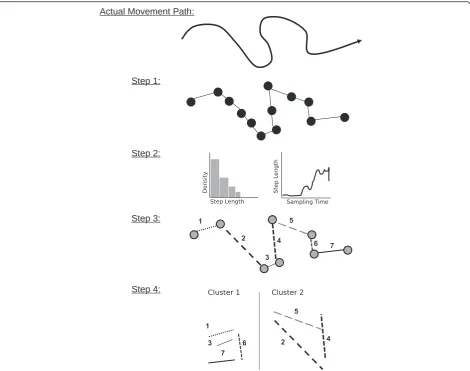
Usually, we cannot observe the complete, continuous movement path of an animal. Instead, we sample a set of discrete relocations to approximate the animals’ actual movement path [16] (Step 1 in Fig. 1). The resulting se-quence of consecutive records of the location of the ani-mal (e.g., spatial coordinates, ordered by time) is termed a movement track or trajectory [17]. How well a trajec-tory reflects the actual movement path of an animal de-pends on the sampling regime as well as the recording systems (GPS, Argos, VHF, light-level geolocation), which influences the spatial accuracy and frequency of relocations.
In path-level movement data, consecutive relocations are either sorted by an ordering factor, for example as the result of direct tracking or following of an animal [18, 19] or by the time at which the relocations were re-corded [16, 20]. Sampling frequency influences the reso-lution of the data and the level of inferential detail that can be obtained [5, 21, 22]. For example, shorter tem-poral intervals allow detailed insight into fine-scale be-haviors, but are more sensitive to sampling errors (e.g., spatial inaccuracies of relocations). In contrast, move-ments sampled at longer temporal intervals can only be interpreted on a broader scale (e.g., encamped vs. disper-sal movements). Additionally, recorded relocations can be spurious or lack spatial accuracy due to habitat in-duced sampling errors [23–26]. Importantly, trajectories also differ with regard to their regularity of the time in-tervals between successive steps. Irregular data com-monly results from missing relocation fixes or varying sampling frequencies throughout a study period (e.g., [27]). Further, irregular intervals between relocation samples can stem from different behaviors of the study species. For example, relocation devices applied with marine animals can usually provide the measured pos-ition data only when the species is close to the surface [28–30].
Basics of path segmentation
We use the term segmentation as a general paraphrase for determining changes in an animal's movement be-havior based on the observed trajectory. The process of segmentation involves the partitioning of a trajectory, τ, into a number of Ksubtrajectories (τ1, τ2, …, τK) called
segments (Steps 1–3 in Fig. 1; see also [31, 32]). Path segmentation can be accomplished directly, by designat-ing each observation to different states or clusters (e.g., [21, 33]). However, path segmentation commonly relies on detecting significant changes (so called change- or breaking-points) in the trajectory as cut-offs for separat-ing the trajectory into distinct segments (e.g., [28]). For this, a variety of path characteristics can be derived from
the trajectory, for example the step length or velocity. These path characteristics should accurately capture movement patterns and allow the detection of changes in these patterns. Given the importance of these path charac-teristics for successfully segmenting movement paths, we discuss them in more detail in the next section.
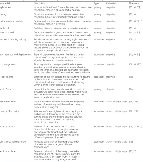
Path characteristics
The various path characteristics used by current seg-mentation methods are summarized in Table 1. These characteristics have also been called movement metrics, movement parameters, path-signals or indices in the lit-erature, and should convey relevant information about individual movement behaviors [31, 34, 35]. The majority of path characteristics are derived from consecutive relo-cations (stepwise), for example the speed of travel. How-ever, some signals are calculated across multiple
relocations, for example the straightness of a trajectory (Table 1).
Dodge et al. [34] distinguished primitive path parame-ters from primary and secondary derived parameparame-ters. The information on the absolute spatial position (e.g., xy-coordinates) and the temporal dimension (time stamp) provide the primitive signals from which other parameters can be derived. For example, displacement and step length (see Table 1) are primary derivatives of the position parameter, whereas time lag (duration) is derived from the temporal primitive.
Path-signals exclusively based on spatial criteria are particularly sensitive to sampling intervals and errors [16, 21]. However, other signals such as the persistence or turning velocity avoid possible biases caused by vary-ing samplvary-ing intervals by relatvary-ing speed to the observed turning angles. Furthermore, signals such as the first
Fig. 1Overview of important steps throughout a segmentation analysis. In general, the actual continuous movement path of an organism is
sampled as a set of consecutive relocations (Step 1; e.g., field work). Step 2: exploratory and descriptive analyses of path characteristics exploring and visualizing of the data structure. Step 3: applying one or several path segmentation method(s) to objectively distinguish different movement states. Step 4: Some methods require the use of clustering and summary statistics to quantify differences in distinguished movement states, and to facilitate biological interpretation in terms of behavioral modes
passage [36] and residence time [31] constitute summary properties accounting for the temporal scales within the movement paths and can be seen as secondary deriva-tives of the distance and duration signals.
Table 1 also lists characteristics which are calculated over multiple relocations and can be applied to de-scribe the signals of single segments, certain
sub-samples of trajectories, or entire trajectories. Such summary signals like the straightness index [37], sinu-osity [38] and the fractal dimension [39] provide in-formation on the spatial complexity of a given path segment and can be used to cluster segments into groups that are similar with respect to movement complexity (Step 4 in Fig. 1). Sinuosity constitutes Table 1Currently applied path characteristics. Different signals or parameters can be calculated either based on consecutive relocations within a trajectory (“stepwise”) or for multiple relocations such as identified path-segments (“across multiple steps”)
Characteristic Description Type Calculation Reference
Displacement Increment of the X and Y values between two consecutive relocations, change in absolute spatial position
primary stepwise [16,34,68]
Time lag Duration / increment in time between consecutive relocations (usually determined by sampling regime)
primary stepwise [16,34]
Turning angles / heading Relative and absolute turning angles between consecutive relocations, change in direction
primary stepwise [16,20,37,122]
Step length Euclidean distance between two consecutive relocations primary stepwise [16,34] Velocity / speed Distance traveled in a given time interval between two
relocations; less sensitive to missing data than step length
primary stepwise [16,28,34]
Persistence / turning velocity Transformations of speed and turning angle: persistence velocity represents the tendency and degree of a movement to persist in a certain direction. Turning velocity shows the tendency of a movement to turn in a perpendicular/opposite direction
secondary stepwise [28,35]
Net / mean squared displacement Squared displacement between the first and current relocation of the trajectory; applied to characterize diffusion behavior or migration patterns
secondary stepwise [16,20,84]
First passage time Time required for crossing a predefined endpoint based on a circle (radius) around a starting relocation. Sums the times of all forward and backwards relocations within the radius; index of area-restricted search behavior
secondary stepwise [31,36,123]
Residence time Extension of the first passage time accounting for returns of the animal in a given area. Sums the times of all relocations (backwards and forwards) of a trajectory within a given vicinity around a relocation.
secondary stepwise [31]
Pseudo-Azimuth Recalculates the basic azimuth value at the midpoint between two consecutive steps to range within 0 and 360. Can be used as indicators for movements with same or parallel directions.
primary stepwise [124]
Straightness index Ratio of Euclidean distance between the beginning and end of a trajectory and the total path length (sum of all step lengths)
secondary across multiple steps [35,123]
Sinuosity / Tortuosity Adaptions of the straightness index analyzing the probabilistic distributions of the changes in the turning angles and the beeline distance between the start and end points of the trajectory; index of path orientation
secondary across multiple steps [38,125]
Fractal dimension Measure of path tortuosity; non-Euclidean dimension of the trajectory varying between one (completely straight) and two (tortuous, completely spanning two-dimensional space); different implementations exist
secondary across multiple steps [39,126–128]
Multi-scale straightness index Repeated calculation of the straightness index of a trajectory over a range of different temporal scales
secondary across multiple steps [76]
Area interest index Repeated calculation of the straightness index for a limited size of a sliding window along the trajectory. With each repetition, the number of relocations within the trajectory is reduced
secondary across multiple steps [76,77]
another example of a secondary derivative of the step length signal [34].
Overall, a large number of different measures can be used to describe path characteristics and a chosen par-ameter should ideally convey relevant information about the underlying movement behavior [31]. This requires a good understanding of the species and a precise defin-ition of research questions, and should also involve ex-tensive exploratory analyses to understand the structure of obtained relocation data and to test the feasibility of different segmentation approaches (Step 2 in Fig. 1; see also below and [35]).
Finding and interpreting segments
Regardless of how and which path characteristics are quantified, significant changes within these signals are then used to determine the K-1 break-points (τ*1, …,
τ*K-1) which can be used to divide the trajectory into K segments (Step 3 in Fig. 1). Although preliminary visual analyses can provide useful indications about a meaning-ful value forK, an objective, data driven way is desirable. Therefore, path segmentation often involves quantitative approaches for detecting an unknown number of seg-ments within a given trajectory, and many of these ap-proaches have originated in non-ecological disciplines (e.g., [40]). This is an important point, as many segmen-tation methods only provide information on significant change-points along the trajectory, without any further ecological context. Thus, it is often not trivial or even possible to directly associate the individual segments to specific activities and behaviors [41]. To facilitate the ecological and ethological interpretation of the defined segments, some methods require subsequent analyses to classify the determined segments based on different de-scriptive parameters or summary statistics (Step 4 in Fig. 1). For example, either the mean values of stepwise characteristics or multi-step summary parameters, such as the straightness index (see Table 1), of the segments can be further analyzed in an additional classification analysis (e.g., [41]). This generates clusters of segments that are similar with respect to relevant path parameters (e.g. calculated across multiple steps, Table 1), which can help to identify underlying movement patterns and asso-ciated behaviors. For example, short, meandering move-ment segmove-ments during within-patch foraging vs. long, straight segments during inter-patch movements [42, 43]. Other methods determine the state (also called class or cluster) of each individual relocation directly and no further classification is necessary [21, 33].
In sum, path segmentation involves at least three and sometimes four major steps (Fig. 1). In the fol-lowing, we focus on the third step, in which signals derived from trajectories are used to objectively define movement segments.
Overview of path segmentation methods
Types of methodological approaches
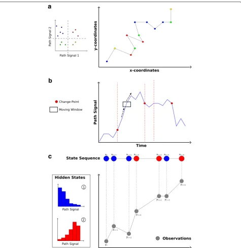
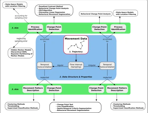
Methods for path segmentation can be distinguished or classified using many different criteria, for example based on their underlying statistical framework (e.g., maximum-likelihood versus Bayesian; parametric or non-parametric, inference-based etc.). Alternatively, Gurarie et al. [35] recently classified broad types of movement analysis tools based on the analytical tradi-tions they stem from. Since our overview is specifically intended for beginners wanting to apply path segmenta-tion, we do not categorize methods based on their statis-tical properties or analystatis-tical traditions, but instead focus on the practical utility of the analyses, e.g., the research questions that can most readily be answered with a cer-tain approach. Hence, we structure our overview based on three broad types of questions that are commonly ad-dressed using path segmentation.
First, movement patterns within the trajectory can be quantified to test whether different movement compo-nents are identifiable within the data. For example, such ‘movement pattern description’is used to distinguish ac-tive from resting phases (e.g., [44]), or encamped for-aging from traveling movements (e.g., [45]). Second, path segmentation can also be used to locate significant changes in movement behavior and determine the tim-ing of these changes. For example, such ‘change-point detection’has been used to quantify behavioral responses to seasonal environmental changes (e.g., [46]), or to identify the timing of migration events (e.g., [47]). Fi-nally, path segmentation can be used to take a detailed look at the processes underlying observed movement patterns. Such ‘process identification’ can be used to examine the factors influencing diel variation in move-ment rates among individuals (e.g., [48]), or to quantify how sex and reproductive status influence the duration of, and transition among, different behavioral modes [49]. These three broad types of research questions can be matched to three basic categories of analytical ap-proaches for path segmentation (Fig. 2).
Topology-based approaches to describe movement patterns
If the study aim is to quantitatively describe movement patterns, one can use methods that focus on the descrip-tion of geometric properties of the trajectory itself, or on one or several signals calculated from the trajectory. Based on this path topology, movement steps are then assorted into groups that are relatively similar with re-spect to these signals (Fig. 2a). The exact way this is ac-complished depends on the method, but can be achieved either bya) simply grouping individual movement steps based on similarity in topology-based signals, regardless of whether these steps are consecutive (e.g. thresholding
Fig. 2The main study aims of path segmentation and types of methods to address them.aPattern description: Topology-based analyses rely directly on signals calculated from the movement trajectory (e.g. step length and bearing). They combine movement steps into groups based on similarity in the considered path-signals, for example by applying clustering algorithms.bChange-point detection: Time-series analyses assess a path-signal (y-axis) along its time-axis. For example, a moving window (rectangle) can be used to search for points along the time-series where local parameters (e.g. the mean) of the path-signal are significantly different from the global averages of these parameters. Significant change-points are assumed to indicate switches in underlying movement modes or behavioral states, and are used to separate the trajectory into segments (dashed lines).cProcess identification: The majority of the presented state-space models link two stochastic models describing the state process and its observation. For example, the state process could consist of two discrete behavioral states (redandblue). The process model describes how the hidden state (x) emerges based on a Markov process. Therefore, it accounts for the conditional probability of a future state depending on the one of the current relocation. The observation model links the actual observed data (y) at given points in time to the hidden state. As a result, the most probable state of each observation, the switching probabilities between the states, as well as the distributions of the measured path-signals within each state are provided.
or clustering; [21, 45]; orb)identifying changes observed among the signals between successive relocations to de-tect so-called change-points (e.g., spatio-temporal cri-teria segmentation; [32]). These change-points are assumed to correspond to changes in underlying move-ment behavior, therefore separating the trajectory into segments consisting of multiple consecutive steps based on pronounced changes in observed movement charac-teristics. These topology-based methods are mostly non-parametric and rather descriptive. Their application is usually based on predefined hypotheses on how move-ment behaviors might differ among habitats, seasons, times of day, sexes, social status, etc..
Time-series analyses to detect significant change-points If the goal of a study is to detect points in time when a significant change in the movement behavior occurs, path segmentation methods based on time-series ana-lyses can be used. Such time-series anaana-lyses are widely used in ecology and related disciplines (see [50]). In the context of path segmentation, these analyses treat signals calculated from consecutive movement steps as time-ordered observations. Essentially, the majority of these approaches try to find significant change-points along the time axis of the signal-sequence derived from the movement trajectory (Fig. 2b). In contrast to the topology-based approaches that analyze the changes be-tween temporally ordered relocations, most of the time-series methods treat movement patterns as a function of time and can directly account for the temporal correla-tions of the sequential signal data. The time-series ap-proaches sometimes depend on certain information like the maximum number of change-points or the mini-mum length of the detected segments. However, they could also potentially be used to “blindly” search for all possible change-points of a given path-signal sequence.
State-space models to identify underlying processes Finally, to increase our understanding of the behav-ioral processes underlying complex movement pat-terns, methods derived from the state-space modeling framework are most suitable. These state-space models represent a special type of time-series analysis [51] and intend to identify latent or hidden behavioral states based on the observed movement data. The aim is to derive deeper insight into the underlying processes by formulating a movement model that ex-plains observed movement patterns. Within these frameworks, the future state of a system is modeled to depend on its current state through a probabilistic model (see Fig. 2c). Therefore, the models typically assume a so-called Markov process structure, meaning that a hidden future state depends on the state of the current step [52]. Essentially, state-space models
couple two stochastic time-series models, one based on an unobservable state process, and another based on a known observation process [52, 53]. When ap-plied to movement data, state-space models assume that animals have several ‘hidden behavioral states’ with certain characteristics (e.g., path-signals) that can be modeled using stochastic processes (e.g., correlated random walks; [54]). A basic result of a state-space model are the estimated transition probabilities be-tween the considered states. Another outcome is the probability of a given relocation belonging to one of the hidden behavioral states. These probabilities are then used to assign steps to their most probable be-havioral state (Fig. 2c) and to segment the trajectory according to state memberships. Additionally, the transition probabilities can also be linked to different environmental factors to test various hypotheses on behavioral and ecological dependencies of the ob-served movement patterns [54–56]. For example, the transition probabilities can be used to test whether switching between states depends on certain habitat characteristics (see simulation study below).
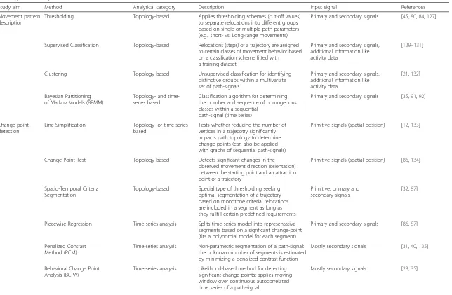
Choosing among methods for path segmentation Multiple methods for path segmentation exist within each of the three types of analytical approaches de-scribed above. Thus, multiple methods exist to answer each of the broad categories of research questions (study aims). Table 2 provides an overview of the available path segmentation methods and lists basic properties, and important background papers for each method. More detailed descriptions and further infor-mation on each path segmentation method, including implementations in the program R [57], can be found in Additional file 1: S1.
Available path segmentation methods vary substan-tially with regard to their demands on data structure and underlying theory. This raises the question of how scien-tists can identify the most appropriate segmentation method(s) for their specific research goals. In the follow-ing, we provide some general guidelines for method se-lection. Additionally, the guidelines are visually summarized in Fig. 3.
Preliminary data analyses
Because the structure and composition of movement data dictate the applicability of certain methods (Fig. 3; blue panel), the first step in any segmentation study should be a preliminary analysis of the available location data. Various analyses can be carried out to gain a better understanding of data properties, but a preliminary ana-lysis for path segmentation should contain at least the following four steps.
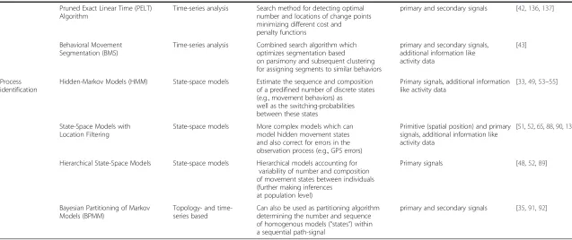
Table 2Characteristics of the methodological approaches for the three different categories of research questions. Different methods for answering the three type of broad research questions (study aims) are listed together with the analytical category they stem from, a short description of each method as well as the considered categories of input path-signals and important references
Study aim Method Analytical category Description Input signal References
Movement pattern description
Thresholding Topology-based Applies thresholding schemes (cut-off values)
to separate relocations into different groups based on single or multiple path parameters (e.g., short- vs. Long-range movements)
Primary and secondary signals [45,80,84,127]
Supervised Classification Topology-based Relocations (steps) of a trajectory are assigned to certain classes of movement behavior based on a classification scheme fitted with a training dataset
Primary and secondary signals, additional information like activity data
[129–131]
Clustering Topology-based Unsupervised classification for identifying
distinctive groups within a multivariate set of path-signals
Primary and secondary signals, additional information like activity data
[21,132]
Bayesian Partitioning of Markov Models (BPMM)
Topology- and time-series based
Classification algorithm for determining the number and sequence of homogenous classes within a sequential
path-signal (time series)
Primary and secondary signals [35,91,92]
Change-point detection
Line Simplification Topology- or time-series
based
Tests whether reducing the number of vertices in a trajecotry significantly impacts path topology to determine change points (can also be applied with graphs of sequential path-signals)
Primitive signals (spatial position) [12,133]
Change Point Test Topology-based Detects significant changes in the
observed movement direction (orientation) between the starting point and an attraction point of a trajectory
Primitive signals (spatial position) [86,134]
Spatio-Temporal Criteria Segmentation
Topology-based Special type of thresholding seeking optimal segmentation of a trajectory based on monotone criteria: relocations are included in a segment as long as they fullfill certain predefined requirements
Primitive, primary and secondary signals
[32,87]
Piecewise Regression Time-series analysis Splits time-series model into representative segments based on a signficant change-point (fits a polynomial model for each segment)
Primary and secondary signals [86,87]
Penalized Contrast Method (PCM)
Time-series analysis Non-parametric segmentation of a path-signal: the unknown number of segments is estimated by minimizing a penalized contrast function
Mostly secondary signals [31,40,135]
Behavioral Change Point Analysis (BCPA)
Time-series analysis Likelihood-based method for detecting significant change points; applies moving window over continuous autocorrelated time series of a path-signal
Mostly secondary signals [28,35]
Edelhoff
et
al.
Moveme
nt
Ecology
(2016) 4:21
Page
8
of
Table 2Characteristics of the methodological approaches for the three different categories of research questions. Different methods for answering the three type of broad research questions (study aims) are listed together with the analytical category they stem from, a short description of each method as well as the considered categories of input path-signals and important references(Continued)
Pruned Exact Linear Time (PELT) Algorithm
Time-series analysis Search method for detecting optimal number and locations of change points minimizing different cost and penalty functions
primary and secondary signals [42,136,137]
Behavioral Movement Segmentation (BMS)
Time-series analysis Combined search algorithm which optimizes segmentation based on parsimony and subsequent clustering for assigning segments to similar behaviors
primary and secondary signals, additional information like activity data
[43]
Process identification
Hidden-Markov Models (HMM) State-space models Estimate the sequence and composition of a predifined number of discrete states (e.g., movement behaviors) as
well as the switching-probabilities between these states
Primary signals, additional information like activity data
[33,49,53–55]
State-Space Models with Location Filtering
State-space models More complex models which can model hidden movement states and also correct for errors in the observation process (e.g., GPS errors)
Primitive (spatial position) and primary signals, additional information like activity data
[51,52,65,88,90,138]
Hierarchical State-Space Models State-space models Hierarchical models accounting for variability of number and composition of movement states between individuals (further making inferences
at population level)
Primary signals [48,52,89]
Bayesian Partitioning of Markov Models (BPMM)
Topology- and time-series based
Can also be used as partitioning algorithm determining the number and sequence of homogenous models (“states”) within a sequential path-signal
primary and secondary signals [35,91,92]
Edelhoff
et
al.
Moveme
nt
Ecology
(2016) 4:21
Page
9
of
1) Sampling regime
Movement data usually varies substantially with regard to the sampling regime, spatial accuracy and temporal resolution. Therefore, preliminary analyses should in-clude checking for regularity of time-intervals between relocations as well as testing for temporal autocorrel-ation of the path-parameter data [16, 58]. Depending on the results of these analyses, several segmentation methods may no longer be suitable (Fig. 3).
2) Data regularity
Irregular data can be the product of missing relocation fixes and varying sampling regimes which can be a chal-lenge, as some of the statistics used to analyze move-ment paths assume regular intervals within the trajectory and are valid only under those circumstances
[28]. Different processing tools can be applied to reloca-tion data in order to fulfill the assumpreloca-tions of regularity. For example, trajectories can be re-discretized [16, 38], which means that relocations can be removed until the remaining data fulfills the requirement of temporal regu-larity (“thinning”). Alternatively, missing relocations can be replaced by applying techniques such as spatial interpolation [12, 59] or dead-reckoning [60–62]. Fur-thermore, only subsets limited to continuous and regu-larly sampled relocations of the original trajectory can be selected for further analyses [16, 38]. Approaches modeling movement in continuous time are also capable of dealing with irregular data structures (e.g., [53, 63]).
Additionally, habitat induced sampling errors and spatial inaccuracies can occur and need to be addressed throughout the preliminary analyses [23–25]. This in-cludes checking the data for extreme outliers or estimat-ing the error of the applied trackestimat-ing technology (e.g.,
Fig. 3Decision guidelines for choosing appropriate segmentation methods. The process should begin with preliminary analyses of the trajectory
data and derived path-parameters (1). Choosing among methods is then first directed by the data structure and sampling regime (2). Capability of the methods to account for temporal autocorrelation further determines the decision process. In the end, study aims and objectives guide the final decision on a given segmentation method (3)
provided by ARGOS systems; [64]). Some types of state-space models include location filtering where such infor-mation can be implemented as a prior in order to esti-mate the true positions of erroneous relocation data (e.g., Kalman Filtering [65–67]).
3) Data visualization and signal distributions
Visual inspection of the movement trajectory can already indicate the existence of different behavioral modes [68–70]. Also, in order to choose appropriate path-signals conveying information on potential changes within the movement behavior, investigations of their variability and distributions (e.g., histograms) should be considered. For example, multi-modality within the path-signal distributions can also indicate the potential existence of different behavioral modes (see applied ex-amples). Further, depending on the intended segmenta-tion method, knowledge on the parameter distribusegmenta-tions is also needed in order to fit movement models within the various types of state-space models [54, 71]. As a substantial part of the methods stem from the time-series framework, time-ordered plotting of the path-signals can indicate the existence of changes in the se-quence over time (see applied examples below). Visual inspection of the variation of the signals over time can provide insight on the ranging and movement behavior. For example, Bunnefeld et al. [72] and Killeen et al. [15] inspected time-ordered values of net-squared displace-ment (Table 1) for single or multiple modality in order to detect potential migratory individuals.
Further, the visual inspection of movement trajectories can help to identify unusual relocations and movements [69, 70]. Thus, visual inspection of the trajectory is im-portant for error checking and can help to refine bio-logical hypotheses to be tested with a given data set.
4) Scales of movement and data transformation
Detectability and observability of changes in move-ment behavior can also change with temporal and spatial scale [18, 73]. There are multiple options of indexes and transformations providing information on the varying spatial and temporal scales of the path characteristics (e.g., trigonometric circle space; [12]). Further, sub-sampling, re-discretization or moving-windows can be applied to alter the temporal grain (e.g. daily, nocturnal, weekly or monthly relocations) in order to summarize the means or variances of path-parameters [22, 29, 74, 75]. Also, multi-step signals (see Table 1) such as the simple straightness index [37] and its different exten-sions [76, 77] can be applied to investigate the variation of path straightness within a trajectory over time and multiple temporal resolutions. Path-parameters such as
the first passage or residence time (Table 1) can be cal-culated at varying spatial and temporal scales and allow further insight in underlying spatial and temporal scales of individual movement behavior [31, 78, 79]. Finally, different transformations of the path parameters can be applied to determine dominant and constant periodic frequency patterns in the movement data. For example, Fourier and wavelet transformations provide valuable insight in periodic structures of movement, such as cir-cadian, seasonal or diurnal rhythms [80–83].
Study aims
After the preliminary analysis of the data structure and relevant path characteristics, choosing appropriate seg-mentation methods is mostly influenced by the aims of the study (Fig. 3; green panels). Thus, depending on the study aims and data structure, different methods can be applied.
1) Movement pattern description
The majority of appropriate methods for quantitatively describing movement patterns are based on the path-topology approaches such as simple threshold or multi-variate classification algorithms (detailed information for each method in Additional file 1: S1). These approaches are least demanding with regard to data properties like regularity and do not require any data transformations as they make minimal assumptions about underlying data structures, movement models, or behavioral states. However, they can be valuable exploratory tools for deter-mining the potential number of different behavioral states within the observed movement data (e.g., [21, 45, 84]). Furthermore, the methods can be applied for testing cer-tain hypotheses on how particular path-signals change with different behaviors or at certain time-periods. There-fore, for some study aims it might be sufficient to split movements into two or more different behavioral states (e.g., long- vs. short-range movements) based on a thresh-old within a selected path-signal (e.g., step length; [85]). Similarly, the time when the relocations were recorded could be used to distinguish different types of behavior (e.g., daytime vs. nocturnal movements).
In sum, methods for pattern description can be ap-plied to gain insight on potential behavioral states and even for detecting potential drivers of the observed pat-terns (e.g., nocturnal movement behaviors with longer step length). However, the considered path-signals have to be chosen carefully and according to expected changes in movement behaviors and underlying behav-iors [21, 35]. Furthermore, due to their relative simpli-city, topology-based methods offer little explanatory power and are usually not suitable for analyzing complex movement patterns [35].
2) Change-point detection
The second example of a general study aim is the de-termination of important (significant) change-points in the movement behavior or trajectory of an animal. The presented approaches either focus on the path-topology or on a time-series of a path-signal. In both cases, the sequential relationship between consecutive relocations is accounted for.
The relevant topology-based methods either focus on the changes within the absolute spatial position (e.g., the change point test [86]; Table 2) or different path-signals and their shape along the trajectory (e.g., using Spatio-Temporal Criteria Segmentation [87]; Fig. 3). However, the change-points resulting from the topology-based methods usually do not provide any information on the significance of the observed changes within the data composition. If identifying significant change-points is the aim, for example, to detect the onset of migratory events, then methods from the time-series category are the better choice, as they specifically estimate the signifi-cance of changes within a time-ordered data sequence (Fig. 2b). The majority of time-series approaches are capable of accounting for temporal autocorrelation within the data sequence which can be an important ad-vantage, because non-independence of relocations is a challenge for many standard statistics [28]. As can be seen in our example, the autocorrelation structure of the data can also contain valuable information about the underlying behavioral states [13]. As a caveat, most time-series methods show higher demands on data prop-erties, especially regularity of the time intervals between relocations (an exception is the behavioral change-point analysis; BCPA). Furthermore, many of the appropriate time-series methods listed in Table 2 depend on one or multiple parameters which need to be defined prior to the analyses such as the size of a moving window (e.g., for the behavioral change point analysis; [28]) or the minimum number of relocations within a determined segment (e.g., for the penalized contrast method; [40]). Therefore, several assumptions, about the number of po-tential changes or the length of a behavioral state, need to be made before setting these parameters, which in-creases the susceptibility to errors and bias and limits reproducibility.
In contrast to that, topology-based methods for change-point detection are less dependent on such par-ameter settings and mostly focus on changes within the spatial composition of the trajectory. However, the scale at which these methods can detect changes in movement behavior is highly dependent on the temporal resolution of the data. Relocations recorded at higher frequencies can provide more detailed information on fine-scale be-haviors. Low frequencies usually limit the scale at which
the topology-based algorithms can determine changes in the underlying behavior [17, 86].
Time-series approaches are usually less sensitive to the temporal sampling frequency of the data for detecting change-points when appropriate input signals conveying meaningful information are used (e.g., persistence vel-ocity; [28]). However, time-series based methods need to be chosen carefully as their assumptions on data distri-butions (e.g., Gaussian vs. non-Gaussian time-series) and applied statistics can differ (see Additional file 1: S1 for more details).
3) Underlying process identification
To identify processes underlying complex movement behaviors, various types of state-space models (SSM) are suitable choices. SSMs intend to identify latent states or hidden models based on the observed movement data. In this context, hidden states represent different behav-ioral modes, assuming that they can be described with different parametric distributions of the path character-istics. The majority of SSMs can be interpreted as a multi-state random walk and are usually based on as-sumptions about the density functions of the step length and turning angle distributions [35, 54]. Hierarchical ap-proaches can be used to estimate different numbers and compositions of behavioral states for each of the studied individuals and further draw model inferences at the population level [52, 54, 88, 89]. Another advantage of these models is that some can account explicitly for is-sues of animal movement data, such as irregularities caused by missing relocations and measurement errors (e.g., location filtering [51, 52]). In particular, SSMs fitted with Bayesian estimation techniques allow the integra-tion of prior knowledge on sampling errors [25, 51, 88]. For example, information on the accuracy and quality of the acquired relocation data as provided by the ARGOS system can be implemented in the observational model of such a SSM framework [67, 88, 89]. Importantly, state-space models can integrate the influence of habitat features and other environmental information, such as sea depth or temperature obtained from electronic tag-ging data, on behavioral changes [53, 55, 90]. Therefore, they provide a valuable framework for estimating and comparing the responses of state compositions and their transition probabilities to different covariates [49, 54, 56]. Furthermore, due to their mechanistic basis, many of the SSM methods provide information on the differ-ences in the estimated parameter distributions of the considered movement models. Thus, state-space models can also be used to simulate or predict movement pat-terns under varying environmental settings [51]. The biggest challenge of using state-space models is the ne-cessity to estimate the various model parameters, which
can require mathematically and computationally com-plex procedures [48, 53]. In summary, state-space models offer much flexibility towards a mechanistic un-derstanding of animal movements, because the process models make it possible to fit specific underlying move-ment patterns (e.g., different correlated-random walks) to the observed movements [51, 88].
However, the number of potential states considered within the models usually needs to be determined prior the application [53]. Also, the general composition of the considered movement models within the states has to be predefined. This limits SSM mostly to variations of discrete correlated random walks [54].
Another option for identifying“hidden states”with dif-ferent compositions of movement parameters is the Bayesian partitioning of Markov models (BPMM) [35, 91]. Technically, this approach is not a state-space model but it represents a simple solution for detecting different models within the observed movement data. The method estimates the distributions of a path-signal for a given number of potential states and assigns each relocation to one of them [91, 92]. However, BPMM does not provide any information on the potential processes, the transition probabilities between the detected states, or the potential influence of covariates.
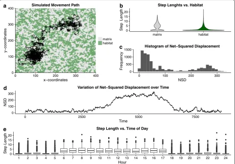
Illustration using simulated data
To illustrate the three types of research questions and related analytical approaches, we next apply one method of each type of analytical approaches to a single data set. For this, we used a simple individual-based simulation model to generate the annual movement track of an animal in R [57]. Details on the simulations and all relevant parameters can be found in Additional file 2: S2. In essence, we simulated an animal that is more active during the day than during the night, moved faster in its habitat than in the matrix (unfavorable habitat) and migrated between two centers of activity (e.g., summering and wintering range). We simulated a movement track for 12 months with relocations taken every hour in a landscape consisting of 400 * 400 cells (Fig. 4a).
For this data set, we were interested in three different research questions. First, we evaluated the hypothesis that the movement intensity of the animal somehow dif-fered between its habitat and the (potentially hostile) matrix, sensu stricto non-habitat. To address this ques-tion, we chose a topology-based method using a thresh-old to distinguish short- from long-range movements and compared the proportions of these two stages within the habitat and matrix. Second, we wanted to assess whether the animal showed a seasonal migration pattern and, if so, to detect the times when migration move-ments occurred throughout the year. For this, we
applied a time-series analysis to segment the movement data based on changes in an observed path-signal. Fi-nally, we assessed whether two different behavioral states could be distinguished and whether the switching prob-ability between those two states could be linked to time of day and habitat. To answer this research question, we used a state-space model approach with two discrete states differing with regard to their dis-tributions of certain path parameters. Before address-ing these research questions, we performed different preliminary analyses to gain insight about data prop-erties and guide the decision process on meaningful path-signals and an appropriate segmentation method for each question (Fig. 3).
Results: preliminary analyses
As pointed out above, preliminary analyses are a funda-mental part of path-level analyses and should be per-formed thoroughly prior to the application of any segmentation approach. As our simulated data set con-sisted of relocation data sampled at an hourly interval, we did not test for regularity of the sampling regime. However, such tests can be performed by inspecting the distribution of the time-lags between the sampled relo-cations (e.g., using histograms). More analyses for check-ing the regularity of a trajectory or testcheck-ing the independence of missing data points are implemented in the adehabitatLT package [92]. In the next step, one should test for potential correlation structures within the observed movement data. We applied different tests based on Dray et al. [58] and detected significant corre-lations between consecutive measures of the step length and also turning angles up to a time lag of five reloca-tions. Therefore, following our guidelines (Fig. 3), we chose among methods accounting for such temporal autocorrelations.
Meaningful path parameters conveying relevant infor-mation about potential changes in movement behavior are essential for a sound path-segmentation analysis. Thus, comparisons of different signals (e.g., primary and secondary derivatives, Table 1) with regard to their dis-tributions and variation over time should be performed in the preliminary analysis. We applied several explora-tory analyses for the step length (due to the hourly sam-pling regime this is also the speed signal), turning angles and net-squared displacement (NSD) signals (more de-tails in Additional file 2: S2). For example, Fig. 4 shows the distributions of NSD and step length as well as their variation over time. The NSD signal provides meaningful information on the ranging behavior of an animal as it represents the distance to the point where the tracking period started. Inspection of this signal over the entire sampling period revealed that there was a steep increase in the values of this parameter followed by a plateau and
decrease until the values were in the same range as at the beginning (Fig. 4d). Further, we observed a trend for a bimodal distribution of NSD (Fig. 4d). As described above, behavioral changes might be detect-able at different temporal scales. Plotting the distribu-tion of step lengths against the time of the day they were recorded revealed that the animal was poten-tially more active during the day as during the night (Fig. 4e). Finally, we used all three path signals, step length (in our case equivalent with speed), turning angles and NSD for the different segmentation approaches.
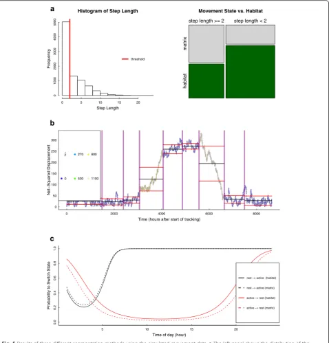
Results: habitat-specific movement patters
We applied a thresholding method to distinguish two different movement patterns within the simulated data-set. A simple cut-off value was used to split relocations into short-range (e.g., encamped) and long-range (e.g., roaming or dispersing) movements. Relocations with an observed step length shorter than two units were
considered short-range movements whereas those with a longer step length were classified as long-range move-ments. As can be seen in Fig. 5a, the proportion of the two movement behaviors varied between habitat and non-habitat. For example, the majority of short-range movements (about 73.3 %) occurred within the habitat of the animal. More than half of the movements (about 58.5 %) outside the habitat stemmed from the long-range behavioral state. Further, a chi-square test indi-cated a significant (non-random) distribution of the two stages between habitat and non-habitat (p< 0.001). Clearly, results highly depend on the chosen threshold value. Therefore, cut-off values need to be chosen care-fully and based on well-reasoned inferences, especially when they are applied with real movement data (see ex-amples in [45, 85]).
Results: timing of migration
In our applied example, we chose the behavioral change-point analysis (BCPA [28]; see Table 2) to demonstrate
0 100 200 300 400
0 100 200 300 400
x−coordinates
y−coordinates
matrix habitat Simulated Movement Path
0 5 10 15 20
matrix habitat
Step Length
Step Lenghts vs. Habitat
0 500 1000 1500
0 100 200 300
NSD
Frequency
Histogram of Net−Squared Displacement
0 100 200 300
0 2500 5000 7500
Time
NSD
Variation of Net−Squared Displacement over Time
0 5 10 15 20
1 2 3 4 5 6 7 8 9 10 11 12 13 14 15 16 17 18 19 20 21 22 23 24
Hour
Step Length
Step Length vs. Time of Day
a
b
c
d
e
Fig. 4Simulated trajectory and results of preliminary analyses.aoverview of the simulated movement path and habitat configuration.b
distributions of observed step lengths within and outside the habitat (matrix) of the tracked animal. Results of preliminary analyses for the net-squared displacement signal including the distribution (c) and the time-series across the entire tracking period (d). Distributions of observed step lengths at different hours of the day (e)
how significant changes can be detected within a time-series of a path-signal in order to find segments of po-tential migratory behavior. We chose the sequence of the net-squared displacement parameter (NSD, Table 1)
as the model input. As can be seen in Fig. 5b) the BCPA determined multiple segments with comparably low net-squared displacement prior to the simulated migration event (from 0 to 3000 h after the start of tracking). That Histogram of Step Length
Step Length
Frequency
0 5 10 15 20
0
1000
2000
3000
4000
5000
threshold
a
Movement State vs. Habitatstep length >= 2 step length < 2
matr
ix
habitat
0 2000 4000 6000 8000
0 50 100 150 200 250 300
Time (hours after start of tracking)
Net−Squared Displacement
ρ ^
0 270
530 800
1100
b
5 10 15 20
0.0
0.2
0.4
0
.6
0.8
1
.0
Time of day (hour)
Probability to Switch State
rest −> active (habitat)
rest −> active (matrix)
active −> rest (habitat)
active −> rest (matrix)
c
Fig. 5Results of three different segmentation methods using the simulated movement data.aThe left panel shows the distribution of the
observed step lengths as well as the applied cut-off value (threshold = 2 units). The proportions of the resulting behavioral states (short- and long-range movements) within and outside of the habitat are shown in the right panel.bResults from the behavioral change point analyses applied with the net-squared displacement signal. The observed time-series was segmented at significant change-points (vertical lines) to distinguish movements within the main ranges of the animal and two migratory periods. The color of the estimated parameterρ^ indicates the level of temporal autocorrelation.cChange in switching probabilities between the two states (resting vs. active) dependent on the different hours of the day. Switching probabilities also differed with regard to whether the animal was in its habitat or not. Black lines indicate the switches from the resting state to the active state. Red lines are showing the switching probabilities from active to resting state
period is followed by a segment with increasing displace-ment and also higher autocorrelation which can be interpreted as potentially migratory behavior. The plat-eau within the NSD time-series (around 4000 to 5500 h after start of tracking) marks the arrival of the simulated animal track in its second range (e.g., summering grounds). The second migratory event is once again de-tected by a segment with decreasing NSD but also high autocorrelation values. Finally, the last two segments have low values of NSD comparable to the beginning in-dicating that the animal has returned to the first range where the tracking was started (e.g., wintering grounds). In summary, the time-series based analysis was success-ful at determining multiple segments, including a dis-tinction of within-range movements from migratory movements, as well as an identification of the starting time of migration.
Results: underlying processes
In the third example, we addressed the question whether the switches between different movement states could be linked to two covariates, the time of the day and whether the animal was within or outside its habitat. We applied a hidden Markov model (HMM; Table 2) with two discrete behavioral states which differed with regard to their means of the step length and turning angle parameter distributions (more details are presented in Additional file 2: S2). The model was fitted using the moveHMM package [93]. The first state consisted of relocations with very low step length values (mean of 0.11 units) and mostly negative turning angles. Therefore, this state was considered to represent resting or sedentary movement behavior. In contrast, the second state comprised of relocations with longer step lengths (mean of 3.4 units) and positive turning angles poten-tially representing active movement phases. The prob-ability for the animal to switch from the resting to the active state was lower during the beginning of the day and increased with daytime (Fig. 5c). The switching-probability from active to resting decreased during daytime and was higher during the night. Fur-ther, the probability to switch from resting to active was slightly higher when the animal was outside its habitat. Complementary to that, the animal was less probable to switch from active to resting when it was in non-habitat (Fig. 5c). Overall, the model output represents the simulated movement behavior which consisted of higher movement activity during the day-time and faster movements outside the habitat. This underlines the high potential of different state-space model approaches for gaining a better understanding of the processes and mechanisms potentially driving the observed movement patterns [35, 51].
Discussion
The aim of movement ecology is to gain a deeper under-standing of the mechanisms and ecological processes shaping organismal movement patterns and their conse-quences for ecology and evolution [4, 5]. The methods presented here can be applied to define behavioral states from the observed movement paths and link these be-havioral states to different environmental covariates to gain an enhanced understanding of the biological pro-cesses influencing the movement behavior of animals [14, 15]. However, there is no single method that can be universally applied to any kind of study scenario. As il-lustrated above, path segmentation methods vary sub-stantially with regard to their demands on data structure and underlying theory. Given this analytical variability, there are certainly several possibilities on how to group and categorize the different methods for path segmenta-tion (e.g., [35]). Here, we chose to contrast different ana-lytical approaches with regard to their applicability for answering certain research questions, rather than their underlying statistical frameworks. Nevertheless, we en-courage researchers interested in applying path segmen-tation methods to read about the statistical details of the different methods (Additional file 1: S1) and consult the original method papers to fully understand the statistical properties of the method(s) they intend to apply.
We used a simulated dataset to demonstrate how our proposed decision process (Fig. 3) can be performed to answer different research questions using methods from the three analytical categories of topology-based, time-series and state-space analyses. Certainly, each of these categories have advantages and disadvantages one has to account for when choosing among them.
The majority of methods focusing on path-topology (Table 2) are purely descriptive and usually just draw new observations based on the tracked movement pat-tern [33, 35]. However, for certain analyses this might already be sufficient to answer the defined research questions. For example, we showed how a relatively sim-ple thresholding approach can be used to distinguish be-tween two extrema of a potential movement behavior (short- vs long-range movements) based on a path char-acteristic and linked them to different habitat configura-tions. Thus, topology-based approaches are useful when specific hypotheses regarding movement patterns can be formulated a priori [21]. Also, topology-based methods are least demanding in terms of data composition and regularity, as they make no specific assumptions about data properties or the distribution of the considered path characteristics. Furthermore, they are analytically the most straightforward and can serve as exploratory tools e.g., for determining the number of potential movement states that could be further analyzed in a more infer-ence- or process-based approach such as a SSM [33].
However, these methods should not generally be applied as end-point analyses since they are mostly ignoring other valuable information like the serial autocorrelation of path parameters.
Time-series based approaches are usually more de-manding with regard to data composition but provide deeper insight to significant changes in movement be-haviors and account for important correlation structures present in movement data [28]. Such methods can easily be used for finding single or multiple change-points in a trajectory to determine the moment of important changes in movement behavior.
State-space models are arguably the most powerful way for analyzing animal movement data, providing a “bottom-up” (holistic) approach where behavioral states and switching probabilities between them are modeled within the same process [51, 52, 55]. However, the esti-mated state configurations are also based on certain model assumptions about the movement properties (e.g., variants of correlated random walks) and the observed pattern in the considered data [53]. Therefore, SSMs do not ultimately convey a biological meaningful differenti-ation between different (“true”) movement behaviors [53, 55]. Furthermore, many of the presented SSMs are quite complex and hence perhaps the most challenging to apply to empirical data. In order to foster the application of state-space models in movement ecology, we encour-age biologists to cooperate with statisticians and mod-elers when designing studies and analyzing data. Such interdisciplinary research teams should refer to the growing number of R packages for fitting state-space models (e.g., [93, 94]; see Additional file 1: S1), and to the increasing number of papers providing practical ad-vice for using these models (e.g. [51, 52, 95]).
Finally, the majority of the presented methods of the time-series and state-space analyses are based on discrete-time models and therefore require regular sam-pling regimes (Fig. 3; [96]). Such data regularity is not al-ways possible to obtain, even though various procedures reaching regular sampling are available (see above). However, there are multiple approaches using diffusion processes which model movements in continuous time and are capable of dealing with irregular data composi-tions [53, 97]. For example, highly infrequently sampled movement data can be analyzed using a spatial HMM with a discrete space structure [52, 98]. Furthermore, methods implementing continuous time processes and estimating switches between different behavioral states were presented by [63, 99–102].
As highlighted by Gurarie et al. [35], preliminary data analysis is a very important part of working with move-ment data, and we emphasize that it will often result in a much deeper understanding of observed patterns, can help to identify optimal analytical approaches for a given
data set, and can eventually lead to more meaningful conclusions. A main focus should be to determine what characteristic of the movement is changing in order to choose optimal path-signals representing these changes. Further, the functional relevant time frames at which the observed species moves and potentially changes its be-havior needs to be assessed carefully [74, 103]. In gen-eral, there are multiple path-signals that are commonly used for certain segmentation methods only. For ex-ample, in the literature the penalized contrast method [104] is almost exclusively applied with either the first passage or residence time parameters (e.g., [31, 47, 105]). However, as outlined above (Table 1) there are multiple options for drawing information from the ob-served trajectory using different path parameters. We suggest that new combinations of path-signals or hybrids of different techniques might lead to valuable insights on movement behavior. For instance, instead of the typ-ically used velocity measures for the BCPA (e.g., persist-ence velocity; [28]) we chose the net-squared displacement parameter as the in input signal to deter-mine the timing of migratory behaviors in our simulated dataset. Different analytical methods can also be com-bined in a multi-stage approach where, in a first step, a movement path is segmented using one of the methods for detecting change-points within the movement data (e.g., a time-series approach like BCPA). In a second step, a clustering algorithm could be applied for deter-mining groups of segments with the potentially same be-havior (e.g., Step 4 in Fig. 1). In a final step, the segments of the different clusters of movement behavior could be linked to various types of environmental data (e.g., using a step-selection analysis [106, 107]). For ex-ample, Zhang et al. [41] applied such a multi-stage ap-proach to determine a number of distinct behaviors within the movement data of little penguins (Eudyptula minor) and compared the location and timing of the be-havioral switches between the sampled individuals. How-ever, throughout this “top-down” process uncertainties of the chosen segmentation method are potentially pro-jected on to the results of the subsequent analyses which could lead to biased results and interpretations. Cur-rently, it is not clear how severe such uncertainties are for subsequent analyses and ecological inferences.
Future research needs
The continuing improvement of tracking devices will provide researchers with long-term movement data at high spatial and temporal resolutions [7]. Additionally, the establishment of collaborative projects and data col-lections will continue to facilitate analyses across many individuals, species, and study areas [4, 108]. To fully realize the potential of this abundant high quality data, powerful analytical techniques are needed. While a