Labview Analysis Concepts Highlighted

LabVIEW

Analysis Concepts

Worldwide Technical Support and Product Information ni.com

National Instruments Corporate Headquarters

11500 North Mopac Expressway Austin, Texas 78759-3504 USA Tel: 512 683 0100

Worldwide Offices

Australia 1800 300 800, Austria 43 0 662 45 79 90 0, Belgium 32 0 2 757 00 20, Brazil 55 11 3262 3599, Canada (Calgary) 403 274 9391, Canada (Ottawa) 613 233 5949, Canada (Québec) 450 510 3055, Canada (Toronto) 905 785 0085, Canada (Vancouver) 514 685 7530, China 86 21 6555 7838, Czech Republic 420 224 235 774, Denmark 45 45 76 26 00, Finland 385 0 9 725 725 11,

France 33 0 1 48 14 24 24, Germany 49 0 89 741 31 30, Greece 30 2 10 42 96 427, India 91 80 51190000, Israel 972 0 3 6393737, Italy 39 02 413091, Japan 81 3 5472 2970, Korea 82 02 3451 3400,

Malaysia 603 9131 0918, Mexico 001 800 010 0793, Netherlands 31 0 348 433 466,

New Zealand 0800 553 322, Norway 47 0 66 90 76 60, Poland 48 22 3390150, Portugal 351 210 311 210, Russia 7 095 783 68 51, Singapore 65 6226 5886, Slovenia 386 3 425 4200, South Africa 27 0 11 805 8197, Spain 34 91 640 0085, Sweden 46 0 8 587 895 00, Switzerland 41 56 200 51 51, Taiwan 886 2 2528 7227, Thailand 662 992 7519, United Kingdom 44 0 1635 523545

Important Information

Warranty

The media on which you receive National Instruments software are warranted not to fail to execute programming instructions, due to defects in materials and workmanship, for a period of 90 days from date of shipment, as evidenced by receipts or other documentation. National Instruments will, at its option, repair or replace software media that do not execute programming instructions if National Instruments receives notice of such defects during the warranty period. National Instruments does not warrant that the operation of the software shall be uninterrupted or error free.

A Return Material Authorization (RMA) number must be obtained from the factory and clearly marked on the outside of the package before any equipment will be accepted for warranty work. National Instruments will pay the shipping costs of returning to the owner parts which are covered by warranty.

National Instruments believes that the information in this document is accurate. The document has been carefully reviewed for technical accuracy. In the event that technical or typographical errors exist, National Instruments reserves the right to make changes to subsequent editions of this document without prior notice to holders of this edition. The reader should consult National Instruments if errors are suspected. In no event shall National Instruments be liable for any damages arising out of or related to this document or the information contained in it. EXCEPTASSPECIFIEDHEREIN, NATIONAL INSTRUMENTSMAKESNOWARRANTIES, EXPRESSORIMPLIED, ANDSPECIFICALLYDISCLAIMSANYWARRANTYOF MERCHANTABILITYORFITNESSFORAPARTICULARPURPOSE. CUSTOMER’SRIGHTTORECOVERDAMAGESCAUSEDBYFAULTORNEGLIGENCEONTHEPARTOF

NATIONAL INSTRUMENTSSHALLBELIMITEDTOTHEAMOUNTTHERETOFOREPAIDBYTHECUSTOMER. NATIONAL INSTRUMENTSWILLNOTBELIABLEFOR DAMAGESRESULTINGFROMLOSSOFDATA, PROFITS, USEOFPRODUCTS, ORINCIDENTALORCONSEQUENTIALDAMAGES, EVENIFADVISEDOFTHEPOSSIBILITY THEREOF. This limitation of the liability of National Instruments will apply regardless of the form of action, whether in contract or tort, including negligence. Any action against National Instruments must be brought within one year after the cause of action accrues. National Instruments shall not be liable for any delay in performance due to causes beyond its reasonable control. The warranty provided herein does not cover damages, defects, malfunctions, or service failures caused by owner’s failure to follow the National Instruments installation, operation, or maintenance instructions; owner’s modification of the product; owner’s abuse, misuse, or negligent acts; and power failure or surges, fire, flood, accident, actions of third parties, or other events outside reasonable control.

Copyright

Under the copyright laws, this publication may not be reproduced or transmitted in any form, electronic or mechanical, including photocopying, recording, storing in an information retrieval system, or translating, in whole or in part, without the prior written consent of National Instruments Corporation.

For a listing of the copyrights, conditions, and disclaimers regarding components used in USI (Xerces C++, ICU, and HDF5), refer to the USICopyrights.chm.

This product includes software developed by the Apache Software Foundation (http://www.apache.org/). Copyright© 1999 The Apache Software Foundation. All rights reserved.

Copyright © 1995–2003 International Business Machines Corporation and others. All rights reserved. NCSA HDF5 (Hierarchical Data Format 5) Software Library and Utilities

Copyright 1998, 1999, 2000, 2001, 2003 by the Board of Trustees of the University of Illinois. All rights reserved.

Trademarks

CVI™_{, LabVIEW}™_{, National Instruments}™_{, NI}™_{, and ni.com}™ _{are trademarks of National Instruments Corporation.}

MATLAB® _{is a registered trademark of The MathWorks, Inc. Other product and company names mentioned herein are trademarks or trade}

names of their respective companies.

Patents

For patents covering National Instruments products, refer to the appropriate location: Help»Patents in your software, the patents.txt file on your CD, or ni .c om /p at en ts.

WARNING REGARDING USE OF NATIONAL INSTRUMENTS PRODUCTS

(1) NATIONAL INSTRUMENTS PRODUCTS ARE NOT DESIGNED WITH COMPONENTS AND TESTING FOR A LEVEL OF RELIABILITY SUITABLE FOR USE IN OR IN CONNECTION WITH SURGICAL IMPLANTS OR AS CRITICAL COMPONENTS IN ANY LIFE SUPPORT SYSTEMS WHOSE FAILURE TO PERFORM CAN REASONABLY BE EXPECTED TO CAUSE SIGNIFICANT INJURY TO A HUMAN.

Contents

About This Manual

Conventions ...xv Related Documentation...xv

P

I

Signal Processing and Signal Analysis

Chapter 1

Introduction to Digital Signal Processing and Analysis in LabVIEW

Chapter 2

Signal Generation

Common Test Signals ...2-1 Frequency Response Measurements ...2-5 Multitone Generation ...2-5 Crest Factor ...2-6 Phase Generation ...2-6 Swept Sine versus Multitone ...2-8 Noise Generation ...2-10 Normalized Frequency...2-12 Wave and Pattern VIs ...2-14 Phase Control...2-14

Chapter 3

Classifying Filters by Impulse Response ... 3-3 Filter Coefficients ... 3-4 Characteristics of an Ideal Filter... 3-5 Practical (Nonideal) Filters... 3-6 Transition Band... 3-6 Passband Ripple and Stopband Attenuation ... 3-7 Sampling Rate ... 3-8 FIR Filters... 3-9 Taps ... 3-11 Designing FIR Filters... 3-11 Designing FIR Filters by Windowing ... 3-14 Designing Optimum FIR Filters Using the Parks-McClellan

Algorithm... 3-15 Designing Equiripple FIR Filters Using the Parks-McClellan

Algorithm... 3-16 Designing Narrowband FIR Filters ... 3-16 Designing Wideband FIR Filters ... 3-19 IIR Filters... 3-19 Cascade Form IIR Filtering... 3-20 Second-Order Filtering ... 3-22 Fourth-Order Filtering ... 3-23 IIR Filter Types ... 3-23 Minimizing Peak Error ... 3-24 Butterworth Filters... 3-24 Chebyshev Filters ... 3-25 Chebyshev II Filters... 3-26 Elliptic Filters ... 3-27 Bessel Filters... 3-28 Designing IIR Filters... 3-30 IIR Filter Characteristics in LabVIEW... 3-31 Transient Response... 3-32 Comparing FIR and IIR Filters... 3-33 Nonlinear Filters ... 3-33 Example: Analyzing Noisy Pulse with a Median Filter... 3-34 Selecting a Digital Filter Design ... 3-35

Chapter 4

Frequency Analysis

Discrete Fourier Transform (DFT) ...4-5 Relationship between N Samples in the Frequency and Time Domains...4-5 Example of Calculating DFT...4-6 Magnitude and Phase Information...4-8 Frequency Spacing between DFT Samples ...4-9 FFT Fundamentals ...4-12

Computing Frequency Components ...4-13 Fast FFT Sizes ...4-14 Zero Padding ...4-14 FFT VI ...4-15 Displaying Frequency Information from Transforms...4-16 Two-Sided, DC-Centered FFT ...4-17 Mathematical Representation of a Two-Sided, DC-Centered FFT ...4-18 Creating a Two-Sided, DC-Centered FFT...4-19 Power Spectrum ...4-22

Converting a Two-Sided Power Spectrum to a Single-Sided

Power Spectrum...4-23 Loss of Phase Information...4-25 Computations on the Spectrum...4-25 Estimating Power and Frequency...4-25 Computing Noise Level and Power Spectral Density ...4-27 Computing the Amplitude and Phase Spectrums ...4-28 Calculating Amplitude in Vrms and Phase in Degrees ...4-29 Frequency Response Function ...4-30 Cross Power Spectrum...4-31 Frequency Response and Network Analysis ...4-31 Frequency Response Function...4-32 Impulse Response Function...4-33 Coherence Function...4-33 Windowing...4-34 Averaging to Improve the Measurement ...4-35 RMS Averaging...4-35 Vector Averaging ...4-36 Peak Hold ...4-36 Weighting ...4-37 Echo Detection...4-37

Chapter 5

Characteristics of Different Smoothing Windows ... 5-11 Main Lobe ... 5-12 Side Lobes... 5-12 Rectangular (None) ... 5-13 Hanning ... 5-14 Hamming... 5-15 Kaiser-Bessel ... 5-15 Triangle ... 5-16 Flat Top ... 5-17 Exponential ... 5-18 Windows for Spectral Analysis versus Windows for Coefficient Design ... 5-19 Spectral Analysis... 5-19 Windows for FIR Filter Coefficient Design ... 5-21 Choosing the Correct Smoothing Window... 5-21 Scaling Smoothing Windows ... 5-23

Chapter 6

Distortion Measurements

Defining Distortion... 6-1 Application Areas ... 6-2 Harmonic Distortion... 6-2 THD ... 6-3 THD + N ... 6-4 SINAD ... 6-4

Chapter 7

DC/RMS Measurements

Chapter 8

Limit Testing

Setting up an Automated Test System ...8-1 Specifying a Limit ...8-1 Specifying a Limit Using a Formula ...8-3 Limit Testing ...8-4 Applications ...8-6 Modem Manufacturing Example...8-6 Digital Filter Design Example...8-7 Pulse Mask Testing Example ...8-8

P

II

Mathematics

Chapter 9

Curve Fitting

Introduction to Curve Fitting ...9-1 Applications of Curve Fitting ...9-2 General LS Linear Fit Theory...9-3 Polynomial Fit with a Single Predictor Variable ...9-6 Curve Fitting in LabVIEW ...9-7 Linear Fit ...9-8 Exponential Fit ...9-8 General Polynomial Fit...9-8 General LS Linear Fit ...9-9 Computing Covariance ...9-10 Building the Observation Matrix ...9-10 Nonlinear Levenberg-Marquardt Fit ...9-11

Chapter 10

Probability and Statistics

Moment about the Mean ... 10-5 Skewness ... 10-6 Kurtosis... 10-6 Histogram... 10-6 Mean Square Error (mse) ... 10-7 Root Mean Square (rms) ... 10-8 Probability ... 10-8 Random Variables... 10-8 Discrete Random Variables ... 10-9 Continuous Random Variables ... 10-9 Normal Distribution ... 10-10

Computing the One-Sided Probability of a Normally

Distributed Random Variable ... 10-11 Finding x with a Known p... 10-12 Probability Distribution and Density Functions... 10-12

Chapter 11

Linear Algebra

Linear Systems and Matrix Analysis... 11-1 Types of Matrices... 11-1 Determinant of a Matrix... 11-2 Transpose of a Matrix ... 11-3 Linear Independence... 11-3 Matrix Rank ... 11-4 Magnitude (Norms) of Matrices ... 11-5 Determining Singularity (Condition Number) ... 11-7 Basic Matrix Operations and Eigenvalues-Eigenvector Problems... 11-8 Dot Product and Outer Product ... 11-10 Eigenvalues and Eigenvectors ... 11-12 Matrix Inverse and Solving Systems of Linear Equations ... 11-14 Solutions of Systems of Linear Equations ... 11-14 Matrix Factorization ... 11-16 Pseudoinverse... 11-17

Chapter 12

Optimization

Linear Programming ...12-3 Linear Programming Simplex Method...12-4 Nonlinear Programming ...12-4 Impact of Derivative Use on Search Method Selection ...12-5 Line Minimization ...12-5 Local and Global Minima...12-5 Global Minimum...12-6 Local Minimum...12-6 Downhill Simplex Method ...12-6 Golden Section Search Method ...12-7 Choosing a New Point x in the Golden Section ...12-8 Gradient Search Methods ...12-9 Caveats about Converging to an Optimal Solution...12-10 Terminating Gradient Search Methods ...12-10 Conjugate Direction Search Methods...12-11 Conjugate Gradient Search Methods...12-12 Theorem A ...12-12 Theorem B...12-13 Difference between Fletcher-Reeves and Polak-Ribiere ...12-14

Chapter 13

Polynomials

Negative Feedback with a Rational Polynomial Function... 13-12 Positive Feedback with a Rational Polynomial Function ... 13-12 Derivative of a Rational Polynomial Function ... 13-13 Partial Fraction Expansion ... 13-13 Heaviside Cover-Up Method... 13-14 Orthogonal Polynomials ... 13-15 Chebyshev Orthogonal Polynomials of the First Kind ... 13-15 Chebyshev Orthogonal Polynomials of the Second Kind... 13-16 Gegenbauer Orthogonal Polynomials ... 13-16 Hermite Orthogonal Polynomials ... 13-17 Laguerre Orthogonal Polynomials ... 13-17 Associated Laguerre Orthogonal Polynomials ... 13-18 Legendre Orthogonal Polynomials ... 13-18 Evaluating a Polynomial with a Matrix... 13-19 Polynomial Eigenvalues and Vectors ... 13-20 Entering Polynomials in LabVIEW... 13-22

P

III

Point-By-Point Analysis

Chapter 14

Point-By-Point Analysis

Introduction to Point-By-Point Analysis ... 14-1 Using the Point By Point VIs ... 14-2 Initializing Point By Point VIs... 14-2 Purpose of Initialization in Point By Point VIs ... 14-2 Using the First Call? Function... 14-3 Error Checking and Initialization ... 14-3 Frequently Asked Questions... 14-5

What Are the Differences between Point-By-Point Analysis

Analysis Stages of the Train Wheel PtByPt VI...14-13 DAQ Stage ...14-13 Filter Stage ...14-13 Analysis Stage...14-14 Events Stage ...14-15 Report Stage ...14-15 Conclusion...14-16

Appendix A

References

Appendix B

About This Manual

This manual describes analysis and mathematical concepts in LabVIEW. The information in this manual directly relates to how you can use LabVIEW to perform analysis and measurement operations.

Conventions

This manual uses the following conventions:

» The » symbol leads you through nested menu items and dialog box options to a final action. The sequence File»Page Setup»Options directs you to pull down the File menu, select the Page Setup item, and select Options

from the last dialog box.

This icon denotes a note, which alerts you to important information.

bold Bold text denotes items that you must select or click in the software, such as menu items and dialog box options. Bold text also denotes parameter names.

italic Italic text denotes variables, emphasis, a cross reference, or an introduction

to a key concept. This font also denotes text that is a placeholder for a word or value that you must supply.

monospace Text in this font denotes text or characters that you should enter from the keyboard, sections of code, programming examples, and syntax examples. This font is also used for the proper names of disk drives, paths, directories, programs, subprograms, subroutines, device names, functions, operations, variables, filenames, and extensions.

Related Documentation

The following documents contain information that you might find helpful as you read this manual:

• LabVIEW Measurements Manual

• The Fundamentals of FFT-Based Signal Analysis and Measurement in

LabVIEW and LabWindows™_/CVI™ _{Application Note, available on}

• LabVIEW Help, available by selecting Help»VI, Function, & How-To Help

• LabVIEW User Manual

• Getting Started with LabVIEW

• On the Use of Windows for Harmonic Analysis with the Discrete

Part I

Signal Processing and Signal Analysis

This part describes signal processing and signal analysis concepts.

• Chapter 1, Introduction to Digital Signal Processing and Analysis in LabVIEW, provides a background in basic digital signal processing and an introduction to signal processing and measurement VIs in LabVIEW.

• Chapter 2, Signal Generation, describes the fundamentals of signal generation.

• Chapter 3, Digital Filtering, introduces the concept of filtering, compares analog and digital filters, describes finite infinite response (FIR) and infinite impulse response (IIR) filters, and describes how to choose the appropriate digital filter for a particular application.

• Chapter 4, Frequency Analysis, describes the fundamentals of the discrete Fourier transform (DFT), the fast Fourier transform (FFT), basic signal analysis computations, computations performed on the power spectrum, and how to use FFT-based functions for network measurement.

• Chapter 6, Distortion Measurements, describes harmonic distortion, total harmonic distortion (THD), signal noise and distortion (SINAD), and when to use distortion measurements.

• Chapter 7, DC/RMS Measurements, introduces measurement analysis techniques for making DC and RMS measurements of a signal.

1

Introduction to Digital Signal

Processing and Analysis in

LabVIEW

Digital signals are everywhere in the world around us. Telephone companies use digital signals to represent the human voice. Radio, television, and hi-fi sound systems are all gradually converting to the digital domain because of its superior fidelity, noise reduction, and signal processing flexibility. Data is transmitted from satellites to earth ground stations in digital form. NASA pictures of distant planets and outer space are often processed digitally to remove noise and extract useful

information. Economic data, census results, and stock market prices are all available in digital form. Because of the many advantages of digital signal processing, analog signals also are converted to digital form before they are processed with a computer.

This chapter provides a background in basic digital signal processing and an introduction to signal processing and measurement VIs in LabVIEW.

The Importance of Data Analysis

The importance of integrating analysis libraries into engineering stations is that the raw data, as shown in Figure 1-1, does not always immediately convey useful information. Often, you must transform the signal, remove noise disturbances, correct for data corrupted by faulty equipment, or compensate for environmental effects, such as temperature and humidity.

By analyzing and processing the digital data, you can extract the useful information from the noise and present it in a form more comprehensible than the raw data, as shown in Figure 1-2.

Figure 1-2. Processed Data

The LabVIEW block diagram programming approach and the extensive set of LabVIEW signal processing and measurement VIs simplify the development of analysis applications.

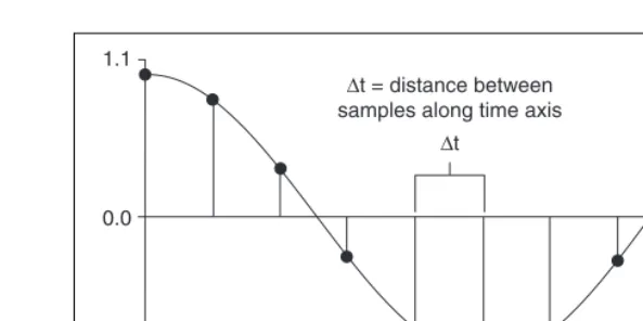
Sampling Signals

Measuring the frequency content of a signal requires digitalization of a continuous signal. To use digital signal processing techniques, you must first convert an analog signal into its digital representation. In practice, the conversion is implemented by using an analog-to-digital (A/D) converter. Consider an analog signal x(t) that is sampled every ∆t seconds. The time interval ∆t is the sampling interval or sampling period. Its reciprocal, 1/∆t, is the sampling frequency, with units of samples/second. Each of the discrete values of x(t) at t = 0, ∆t, 2∆t, 3∆t, and so on, is a sample. Thus,x(0), x(∆t), x(2∆t), …, are all samples. The signal x(t) thus can be represented by the following discrete set of samples.

{x(0), x(∆t), x(2∆t), x(3∆t), …, x(k∆t), …}

Figure 1-3. Analog Signal and Corresponding Sampled Version The following notation represents the individual samples.

x[i] = x(i∆t)

for

i = 0, 1, 2, …

If N samples are obtained from the signal x(t), then you can represent x(t) by the following sequence.

X = {x[0], x[1], x[2], x[3], …, x[N–1]}

The preceding sequence representing x(t) is the digital representation, or the sampled version, of x(t). The sequence X= {x[i]}is indexed on the integer variable i and does not contain any information about the sampling rate. So knowing only the values of the samples contained in X gives you no information about the sampling frequency.

One of the most important parameters of an analog input system is the frequency at which the DAQ device samples an incoming signal. The sampling frequency determines how often an A/D conversion takes place. Sampling a signal too slowly can result in an aliased signal.

1.1

0.0

–1.1

0.0 0.1 0.2 0.3 0.4 0.5 0.6 0.7 0.8 0.9 1.0

∆t = distance between samples along time axis

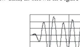
Aliasing

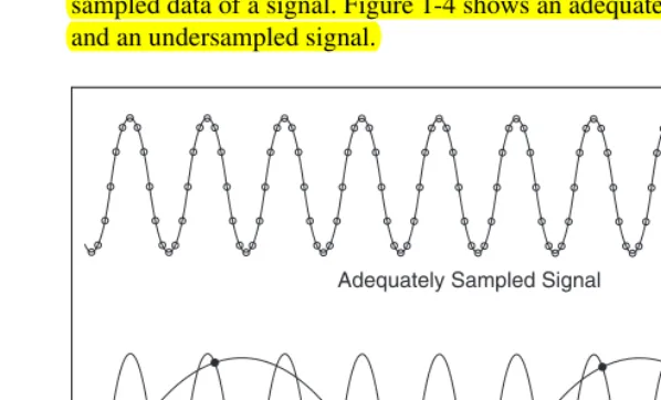
An aliased signal provides a poor representation of the analog signal. Aliasing causes a false lower frequency component to appear in the sampled data of a signal. Figure 1-4 shows an adequately sampled signal and an undersampled signal.

Figure 1-4. Aliasing Effects of an Improper Sampling Rate

In Figure 1-4, the undersampled signal appears to have a lower frequency than the actual signal—three cycles instead of ten cycles.

Increasing the sampling frequency increases the number of data points acquired in a given time period. Often, a fast sampling frequency provides a better representation of the original signal than a slower sampling rate.

For a given sampling frequency, the maximum frequency you can accurately represent without aliasing is the Nyquist frequency. The Nyquist frequency equals one-half the sampling frequency, as shown by the following equation.

,

where f is the Nyquist frequency and f is the sampling frequency. Adequately Sampled Signal

Aliased Signal Due to Undersampling

f_N fs

frequency components below the Nyquist frequency. For example, a component at frequency fN < f0 < fs appears as the frequency fs – f0.

Figures 1-5 and 1-6 illustrate the aliasing phenomenon. Figure 1-5 shows the frequencies contained in an input signal acquired at a sampling frequency, fs, of 100 Hz.

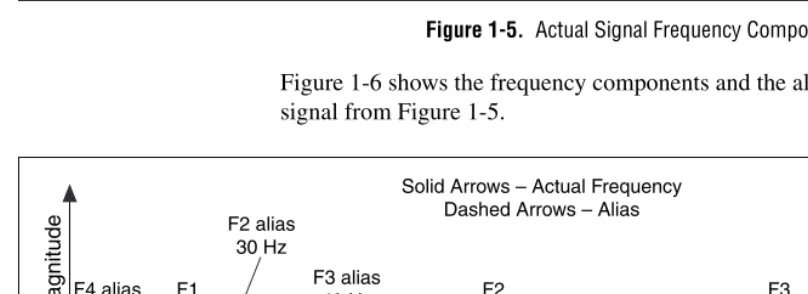
Figure 1-5. Actual Signal Frequency Components

Figure 1-6 shows the frequency components and the aliases for the input signal from Figure 1-5.

Figure 1-6. Signal Frequency Components and Aliases

In Figure 1-6, frequencies below the Nyquist frequency of fs/2 = 50 Hz are sampled correctly. For example, F1 appears at the correct frequency. Frequencies above the Nyquist frequency appear as aliases. For example, aliases for F2, F3, and F4 appear at 30 Hz, 40 Hz, and 10 Hz, respectively.

F1 25 Hz F2 70 Hz F3 160 Hz F4 510 Hz

ƒ_s/2=50 Nyquist Frequency

ƒ_s=100 Sampling Frequency 500 0 Frequency Magnitude F1 25 Hz F2 70 Hz F3 160 Hz F4 510 Hz

ƒ_s/2=50 Nyquist Frequency

ƒ_s=100 Sampling Frequency 500 0 Frequency Magnitude F4 alias 10 Hz F2 alias 30 Hz F3 alias 40 Hz

The alias frequency equals the absolute value of the difference between the closest integer multiple of the sampling frequency and the input frequency, as shown in the following equation.

where AF is the alias frequency, CIMSF is the closest integer multiple of the sampling frequency, and IF is the input frequency. For example, you can compute the alias frequencies for F2, F3, and F4 from Figure 1-6 with the following equations.

Increasing Sampling Frequency to Avoid Aliasing

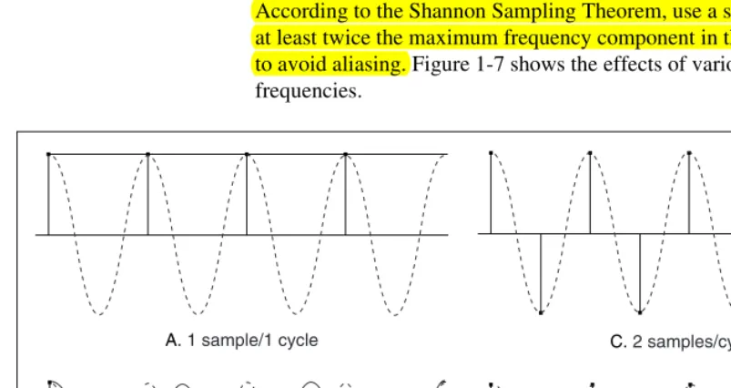
According to the Shannon Sampling Theorem, use a sampling frequency at least twice the maximum frequency component in the sampled signal to avoid aliasing. Figure 1-7 shows the effects of various sampling frequencies.

AF = CIMSF IF–

Alias F2 = 100 70– = 30 Hz Alias F3 = ( )2 100 160– = 40 Hz Alias F4 = ( )5 100 510– = 10 Hz

A. 1 sample/1 cycle

B. 7 samples/4 cycles

C. 2 samples/cycle

In case A of Figure 1-7, the sampling frequency fs equals the frequency f of the sine wave. fs is measured in samples/second. f is measured in cycles/second. Therefore, in case A, one sample per cycle is acquired. The reconstructed waveform appears as an alias at DC.

In case B of Figure 1-7, fs= 7/4f, or 7 samples/4 cycles. In case B, increasing the sampling rate increases the frequency of the waveform. However, the signal aliases to a frequency less than the original signal—three cycles instead of four.

In case C of Figure 1-7, increasing the sampling rate to fs = 2f results in the digitized waveform having the correct frequency or the same number of cycles as the original signal. In case C, the reconstructed waveform more accurately represents the original sinusoidal wave than case A or case B. By increasing the sampling rate to well above f, for example,

fs= 10f= 10 samples/cycle, you can accurately reproduce the waveform. Case D of Figure 1-7 shows the result of increasing the sampling rate to fs= 10f.

Anti-Aliasing Filters

In the digital domain, you cannot distinguish alias frequencies from the frequencies that actually lie between 0 and the Nyquist frequency. Even with a sampling frequency equal to twice the Nyquist frequency, pickup from stray signals, such as signals from power lines or local radio stations, can contain frequencies higher than the Nyquist frequency. Frequency components of stray signals above the Nyquist frequency might alias into the desired frequency range of a test signal and cause erroneous results. Therefore, you need to remove alias frequencies from an analog signal before the signal reaches the A/D converter.

Figure 1-8 shows both an ideal anti-alias filter and a practical anti-alias filter. The following information applies to Figure 1-8:

• f1 is the maximum input frequency.

• Frequencies less than f1 are desired frequencies.

• Frequencies greater than f1 are undesired frequencies.

Figure 1-8. Ideal versus Practical Anti-Alias Filter

An ideal anti-alias filter, shown in Figure 1-8a, passes all the desired input frequencies and cuts off all the undesired frequencies. However, an ideal anti-alias filter is not physically realizable.

Figure 1-8b illustrates actual anti-alias filter behavior. Practical anti-alias filters pass all frequencies <f1 and cut off all frequencies >f2. The region between f1and f2 is the transition band, which contains a gradual attenuation of the input frequencies. Although you want to pass only signals with frequencies <f1, the signals in the transition band might cause aliasing. Therefore, in practice, use a sampling frequency greater than two times the highest frequency in the transition band. Using a sampling frequency greater than two times the highest frequency in the transition band means fs might be more than 2f1.

Converting to Logarithmic Units

On some instruments, you can display amplitude on either a linear scale or a decibel (dB) scale. The linear scale shows the amplitudes as they are. The decibel is a unit of ratio. The decibel scale is a transformation of the linear scale into a logarithmic scale.

Filter Output

f1 Frequency

Transition Band

a. Ideal Anti-alias Filter b. Practical Anti-alias Filter

Filter Output

The following equations define the decibel. Equation 1-1 defines the decibel in terms of power. Equation 1-2 defines the decibel in terms of amplitude.

, (1-1)

where P is the measured power, Pris the reference power, and is the

power ratio.

, (1-2)

where A is the measured amplitude, Ar is the reference amplitude, and is the voltage ratio.

Equations 1-1 and 1-2 require a reference value to measure power and amplitude in decibels. The reference value serves as the 0 dB level. Several conventions exist for specifying a reference value. You can use the following common conventions to specify a reference value for calculating decibels:

• Use the reference one volt-rms squared for power, which yields the unit of measure dBVrms.

• Use the reference one volt-rms (1 Vrms) for amplitude, which yields the unit of measure dBV.

• Use the reference 1 mW into a load of 50 Ω for radio frequencies where 0 dB is 0.22 Vrms, which yields the unit of measure dBm.

• Use the reference 1 mW into a load of 600 Ω for audio frequencies where 0 dB is 0.78 Vrms, which yields the unit of measure dBm.

When using amplitude or power as the amplitude-squared of the same signal, the resulting decibel level is exactly the same. Multiplying the decibel ratio by two is equivalent to having a squared ratio. Therefore, you obtain the same decibel level and display regardless of whether you use the amplitude or power spectrum.

Displaying Results on a Decibel Scale

Amplitude or power spectra usually are displayed on a decibel scale. Displaying amplitude or power spectra on a decibel scale allows you to view wide dynamic ranges and to see small signal components in the presence of large ones. For example, suppose you want to display a signal containing amplitudes from a minimum of 0.1 V to a maximum of 100 V

dB 10 ₁₀P

P_r ---log = P P_r

---dB 20 _10AA

r ---log = A A_r

---1V_rms2

on a device with a display height of 10 cm. Using a linear scale, if the device requires the entire display height to display the 100 V amplitude, the device displays 10 V of amplitude per centimeter of height. If the device displays 10 V/cm, displaying the 0.1 V amplitude of the signal requires a height of only 0.1 mm. Because a height of 0.1 mm is barely visible on the display screen, you might overlook the 0.1 V amplitude component of the signal. Using a logarithmic scale in decibels allows you to see the 0.1 V amplitude component of the signal.

Table 1-1 shows the relationship between the decibel and the power and voltage ratios.

Table 1-1 shows how you can compress a wide range of amplitudes into a small set of numbers by using the logarithmic decibel scale.

Table 1-1. Decibels and Power and Voltage Ratio Relationship

dB Power Ratio Amplitude Ratio

+40 10,000 100

+20 100 10

+6 4 2

+3 2 1.4

0 1 1

–3 1/2 1/1.4

–6 1/4 1/2

–20 1/100 1/10

2

Signal Generation

The generation of signals is an important part of any test or measurement system. The following applications are examples of uses for signal generation:

• Simulate signals to test your algorithm when real-world signals are not available, for example, when you do not have a DAQ device for obtaining real-world signals or when access to real-world signals is not possible.

• Generate signals to apply to a digital-to-analog (D/A) converter.

This chapter describes the fundamentals of signal generation.

Common Test Signals

Common test signals include the sine wave, the square wave, the triangle wave, the sawtooth wave, several types of noise waveforms, and multitone signals consisting of a superposition of sine waves.

The most common signal for audio testing is the sine wave. A single sine wave is often used to determine the amount of harmonic distortion introduced by a system. Multiple sine waves are widely used to measure the intermodulation distortion or to determine the frequency response. Table 2-1 lists the signals used for some typical measurements.

Table 2-1. Typical Measurements and Signals

Measurement Signal

Total harmonic distortion Sine wave

Intermodulation distortion Multitone (two sine waves)

Frequency response Multitone (many sine waves, impulse, chirp), broadband noise

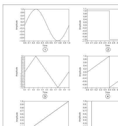
These signals form the basis for many tests and are used to measure the response of a system to a particular stimulus. Some of the common test signals available in most signal generators are shown in Figure 2-1 and Figure 2-2.

Rise time, fall time, overshoot, undershoot

Pulse

Jitter Square wave

Table 2-1. Typical Measurements and Signals (Continued)

Figure 2-1. Common Test Signals 1 Sine Wave

2 Square Wave

3 Triangle Wave 4 Sawtooth Wave

5 Ramp 6 Impulse 1.0 0.8 0.6 0.4 0.2 0.0 –0.2 –0.4 –0.6 –0.8 –1.0

0.0 0.1 0.2 0.3 0.4 0.5 0.6 0.7 0.8 0.9 1.0

Amplitude 1 Time Amplitude Time 1.0 0.8 0.6 0.4 0.2 0.0 –0.2 –0.4 –0.6 –0.8 –1.0

2.0 2.1 2.2 2.3 2.4 2.5 2.6 2.7 2.8 2.9 3.0 1.1 –1.1 2 Amplitude Time 1.0 0.8 0.6 0.4 0.2 0.0 –0.2 –0.4 –0.6 –0.8 –1.0

0.0 0.1 0.2 0.3 0.4 0.5 0.6 0.7 0.8 0.9 1.0

–0.3 Amplitude Time 1.0 0.8 0.6 0.4 0.2 0.0 –0.2 –0.4 –0.6 –0.8 –1.0

0.0 0.1 0.2 0.3 0.4 0.5 0.6 0.7 0.8 0.9 1.0

0.9 0.7 0.5 0.3 0.1 –0.1 –0.5 –0.7 –0.9 3 Amplitude Time 1.0 0.9 0.8 0.7 0.6 0.5 0.4 0.3 0.2 0.1 0.0

0 100 200 300 400 500 600 700 800 900 1000

5 4 Amplitude Time 1.0 0.9 0.8 0.7 0.6 0.5 0.4 0.3 0.2 0.1 0.0

0 100 200 300 400 500 600 700 800 900 1000

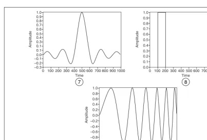
Figure 2-2. More Common Test Signals

The most useful way to view the common test signals is in terms of their frequency content. The common test signals have the following frequency content characteristics:

• Sine waves have a single frequency component.

• Square waves consist of the superposition of many sine waves at odd harmonics of the fundamental frequency. The amplitude of each harmonic is inversely proportional to its frequency.

• Triangle and sawtooth waves have harmonic components that are multiples of the fundamental frequency.

• An impulse contains all frequencies that can be represented for a given sampling rate and number of samples.

• Chirp signals are sinusoids swept from a start frequency to a stop frequency, thus generating energy across a given frequency range.

7 Sinc 8 Pulse 9 Chirp

Amplitude Time 1.0 0.9 0.8 0.6 0.5 0.3 0.1 0.1 –0.3

0 100 200 300 400 500 600 700 800 900 1000 –0.2 –0.1 0.0 0.4 0.7 7 Amplitude Time 1.0 0.9 0.8 0.7 0.5 0.4 0.0

0 100 200 300 400 500 600 700 800 900 1000 0.1 0.2 0.3 0.6 8 Amplitude Time 1.0 0.8 0.6 0.4 0.0 –0.2 –1.0

0 100 200 300 400 500 600 700 800 900 1000 –0.8

–0.6 –0.4 0.2

Frequency Response Measurements

To achieve a good frequency response measurement, the frequency range of interest must contain a significant amount of stimulus energy. Two common signals used for frequency response measurements are the chirp signal and a broadband noise signal, such as white noise. Refer to the Common Test Signals section of this chapter for information about chirp signals. Refer to the Noise Generation section of this chapter for information about white noise.

It is best not to use windows when analyzing frequency response signals. If you generate a chirp stimulus signal at the same rate you acquire the response, you can match the acquisition frame size to the length of the chirp. No window is generally the best choice for a broadband signal source. Because some stimulus signals are not constant in frequency across the time record, applying a window might obscure important portions of the transient response.

Multitone Generation

Except for the sine wave, the common test signals do not allow full control over their spectral content. For example, the harmonic components of a square wave are fixed in frequency, phase, and amplitude relative to the fundamental. However, you can generate multitone signals with a specific amplitude and phase for each individual frequency component.

A multitone signal is the superposition of several sine waves or tones, each with a distinct amplitude, phase, and frequency. A multitone signal is typically created so that an integer number of cycles of each individual tone are contained in the signal. If an FFT of the entire multitone signal is computed, each of the tones falls exactly onto a single frequency bin, which means no spectral spread or leakage occurs.

Crest Factor

The relative phases of the constituent tones with respect to each other determine the crest factor of a multitone signal with specified amplitude. The crest factor is defined as the ratio of the peak magnitude to the RMS value of the signal. For example, a sine wave has a crest factor of 1.414:1.

For the same maximum amplitude, a multitone signal with a large crest factor contains less energy than one with a smaller crest factor. In other words, a large crest factor means that the amplitude of a given component sine tone is lower than the same sine tone in a multitone signal with a smaller crest factor. A higher crest factor results in individual sine tones with lower signal-to-noise ratios. Therefore, proper selection of phases is critical to generating a useful multitone signal.

To avoid clipping, the maximum value of the multitone signal should not exceed the maximum capability of the hardware that generates the signal, which means a limit is placed on the maximum amplitude of the signal. You can generate a multitone signal with a specific amplitude by using different combinations of the phase relationships and amplitudes of the constituent sine tones. A good approach to generating a signal is to choose amplitudes and phases that result in a lower crest factor.

Phase Generation

The following schemes are used to generate tone phases of multitone signals:

• Varying the phase difference between adjacent frequency tones linearly from 0 to 360 degrees

• Varying the tone phases randomly

Varying the phase difference between adjacent frequency tones linearly from 0 to 360 degrees allows the creation of multitone signals with very low crest factors. However, the resulting multitone signals have the following potentially undesirable characteristics:

• The multitone signal is very sensitive to phase distortion. If in the course of generating the multitone signal the hardware or signal path induces non-linear phase distortion, the crest factor might vary considerably.

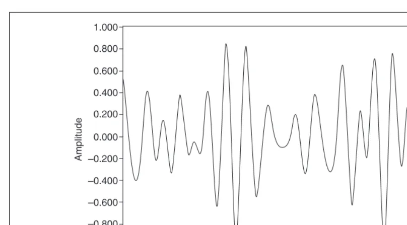
Figure 2-3. Multitone Signal with Linearly Varying Phase Difference between Adjacent Tones

The signal in Figure 2-3 resembles a chirp signal in that its frequency appears to decrease from left to right. The apparent decrease in frequency from left to right is characteristic of multitone signals generated by linearly varying the phase difference between adjacent frequency tones. Having a signal that is more noise-like than the signal in Figure 2-3 often is more desirable.

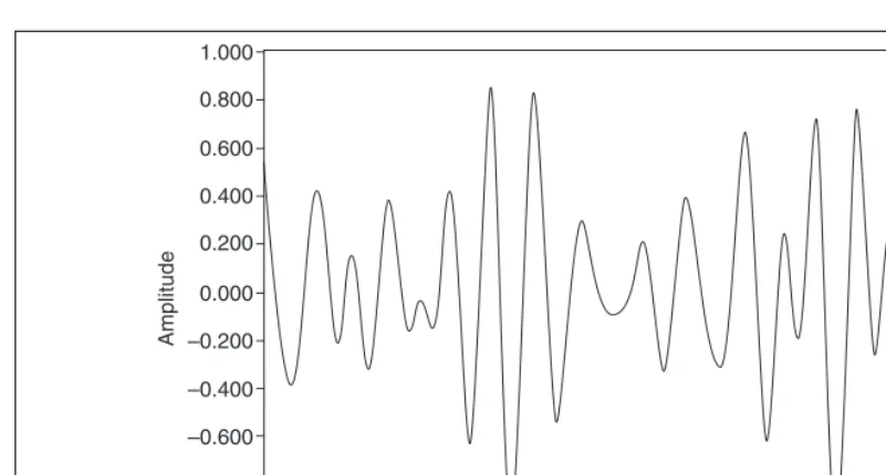
Varying the tone phases randomly results in a multitone signal whose amplitudes are nearly Gaussian in distribution as the number of tones increases. Figure 2-4 illustrates a signal created by varying the tone phases randomly.

1.000

0.800

0.600

0.400

0.200

0.000

–0.200

–0.400

–0.600

–0.800

–1.000

0.000 0.010 0.020 0.030 0.040 0.050 0.060 0.070 0.080 0.090 0.100

Amplitude

Figure 2-4. Multitone Signal with Random Phase Difference between Adjacent Tones In addition to being more noise-like, the signal in Figure 2-4 also is much less sensitive to phase distortion. Multitone signals with the sort of phase relationship shown in Figure 2-4 generally achieve a crest factor between 10 dB and 11 dB.

Swept Sine versus Multitone

To characterize a system, you often must measure the response of the system at many different frequencies. You can use the following methods to measure the response of a system at many different frequencies:

• Swept sine continuously and smoothly changes the frequency of a sine wave across a range of frequencies.

• Stepped sine provides a single sine tone of fixed frequency as the stimulus for a certain time and then increments the frequency by a discrete amount. The process continues until all the frequencies of interest have been reached.

• Multitone provides a signal composed of multiple sine tones.

A multitone signal has significant advantages over the swept sine and 1.000

0.800

0.600

0.400

0.200

0.000

–0.200

–0.400

–0.600

–0.800

–1.000

0.000 0.010 0.020 0.030 0.040 0.050 0.060 0.070 0.080 0.090 0.100

Amplitude

measurement, you must wait for the settling time of the system to end before starting the measurement.

The settling time issue for a swept sine can be even more complex. If the system has low-frequency poles and/or zeroes or high Q-resonances, the system might take a relatively long time to settle. For a multitone signal, you must wait only once for the settling time. A multitone signal containing one period of the lowest frequency—actually one period of the highest frequency resolution—is enough for the settling time. After the response to the multitone signal is acquired, the processing can be very fast. You can use a single fast Fourier transform (FFT) to measure many frequency points, amplitude and phase, simultaneously.

The swept sine approach is more appropriate than the multitone approach in certain situations. Each measured tone within a multitone signal is more sensitive to noise because the energy of each tone is lower than that in a single pure tone. For example, consider a single sine tone of amplitude 10 V peak and frequency 100 Hz. A multitone signal containing 10 tones, including the 100 Hz tone, might have a maximum amplitude of 10 V. However, the 100 Hz tone component has an amplitude somewhat less than 10 V. The lower amplitude of the 100 Hz tone component is due to the way that all the sine tones sum. Assuming the same level of noise, the

signal-to-noise ratio (SNR) of the 100 Hz component is better for the case of the swept sine approach. In the multitone approach, you can mitigate the reduced SNR by adjusting the amplitudes and phases of the tones, applying higher energy where needed, and applying lower energy at less critical frequencies.

Noise Generation

You can use noise signals to perform frequency response measurements or to simulate certain processes. Several types of noise are typically used, namely uniform white noise, Gaussian white noise, and periodic random noise.

The term white in the definition of noise refers to the frequency domain characteristic of noise. Ideal white noise has equal power per unit bandwidth, resulting in a flat power spectral density across the frequency range of interest. Thus, the power in the frequency range from 100 Hz to 110 Hz is the same as the power in the frequency range from 1,000 Hz to 1,010 Hz. In practical measurements, achieving the flat power spectral density requires an infinite number of samples. Thus, when making measurements of white noise, the power spectra are usually averaged, with more number of averages resulting in a flatter power spectrum.

The terms uniform and Gaussian refer to the probability density function (PDF) of the amplitudes of the time-domain samples of the noise. For uniform white noise, the PDF of the amplitudes of the time domain samples is uniform within the specified maximum and minimum levels. In other words, all amplitude values between some limits are equally likely or probable. Thermal noise produced in active components tends to be uniform white in distribution. Figure 2-5 shows the distribution of the samples of uniform white noise.

For Gaussian white noise, the PDF of the amplitudes of the time domain samples is Gaussian. If uniform white noise is passed through a linear system, the resulting output is Gaussian white noise. Figure 2-6 shows the distribution of the samples of Gaussian white noise.

Figure 2-6. Gaussian White Noise

Periodic random noise (PRN) is a summation of sinusoidal signals with the same amplitudes but with random phases. PRN consists of all sine waves with frequencies that can be represented with an integral number of cycles in the requested number of samples. Because PRN contains only integral-cycle sinusoids, you do not need to window PRN before

performing spectral analysis. PRN is self-windowing and therefore has no spectral leakage.

PRN does not have energy at all frequencies as white noise does but has energy only at discrete frequencies that correspond to harmonics of a fundamental frequency. The fundamental frequency is equal to the sampling frequency divided by the number of samples. However, the level of noise at each of the discrete frequencies is the same.

Figure 2-7. Spectral Representation of Periodic Random Noise and Averaged White Noise

Normalized Frequency

In the analog world, a signal frequency is measured in hertz (Hz), or cycles per second. But the digital system often uses a digital frequency, which is the ratio between the analog frequency and the sampling frequency, as shown by the following equation.

Some of the Signal Generation VIs use a frequency input f that is assumed to use normalized frequency units of cycles per sample. The normalized frequency ranges from 0.0 to 1.0, which corresponds to a real frequency range of 0 to the sampling frequency fs. The normalized frequency also wraps around 1.0 so a normalized frequency of 1.1 is equivalent to 0.1. For example, a signal sampled at the Nyquist rate offs/2 means it is sampled twice per cycle, that is, two samples/cycle. This sampling rate corresponds to a normalized frequency of 1/2 cycles/sample = 0.5 cycles/sample. The reciprocal of the normalized frequency, 1/f, gives you the number of times the signal is sampled in one cycle, that is, the number of samples per cycle.

When you use a VI that requires the normalized frequency as an input, you must convert your frequency units to the normalized units of cycles per sample. You must use normalized units of cycles per sample with the following Signal Generation VIs:

• Sine Wave

• Square Wave

• Sawtooth Wave

• Triangle Wave

• Arbitrary Wave

• Chirp Pattern

If you are used to working in frequency units of cycles, you can convert cycles to cycles per sample by dividing cycles by the number of samples generated.

You need only divide the frequency in cycles by the number of samples. For example, a frequency of two cycles is divided by 50 samples, resulting in a normalized frequency of f = 1/25 cycles/sample. This means that it takes 25, the reciprocal of f, samples to generate one cycle of the sine wave.

However, you might need to use frequency units of Hz, cycles per second. If you need to convert from Hz to cycles per sample, divide your frequency in Hz by the sampling rate given in samples per second, as shown in the following equation.

For example, you divide a frequency of 60 Hz by a sampling rate of 1,000 Hz to get the normalized frequency of f = 0.06 cycles/sample.

cycles per second samples per second

--- cycles

sample

Therefore, it takes almost 17, or 1/0.06, samples to generate one cycle of the sine wave.

The Signal Generation VIs create many common signals required for network analysis and simulation. You also can use the Signal Generation VIs in conjunction with National Instruments hardware to generate analog output signals.

Wave and Pattern VIs

The names of most of the Signal Generation VIs contain the word wave or pattern. A basic difference exists between the operation of the two different types of VIs. The difference has to do with whether the VI can keep track of the phase of the signal it generates each time the VI is called.

Phase Control

The wave VIs have a phase in input that specifies the initial phase in degrees of the first sample of the generated waveform. The wave VIs also have a phase out output that indicates the phase of the next sample of the generated waveform. In addition, a reset phase input specifies whether the phase of the first sample generated when the wave VI is called is the phase specified in the phase in input or the phase available in the phase out

output when the VI last executed. A TRUE value for reset phase sets the initial phase to phase in. A FALSE value for reset phase sets the initial phase to the value of phase out when the VI last executed.

3

Digital Filtering

This chapter introduces the concept of filtering, compares analog and digital filters, describes finite impulse response (FIR) and infinite impulse response (IIR) filters, and describes how to choose the appropriate digital filter for a particular application.

Introduction to Filtering

The filtering process alters the frequency content of a signal. For example, the bass control on a stereo system alters the low-frequency content of a signal, while the treble control alters the high-frequency content. Changing the bass and treble controls filters the audio signal. Two common filtering applications are removing noise and decimation. Decimation consists of lowpass filtering and reducing the sample rate.

The filtering process assumes that you can separate the signal content of interest from the raw signal. Classical linear filtering assumes that the signal content of interest is distinct from the remainder of the signal in the frequency domain.

Advantages of Digital Filtering Compared to Analog Filtering

An analog filter has an analog signal at both its input x(t) and its output y(t). Both x(t) and y(t) are functions of a continuous variable t and can have an infinite number of values. Analog filter design requires advanced mathematical knowledge and an understanding of the processes involved in the system affecting the filter.

Digital filters have the following advantages compared to analog filters:

• Digital filters are software programmable, which makes them easy to build and test.

• Digital filters require only the arithmetic operations of multiplication and addition/subtraction.

• Digital filters do not drift with temperature or humidity or require precision components.

• Digital filters have a superior performance-to-cost ratio.

• Digital filters do not suffer from manufacturing variations or aging.

Common Digital Filters

You can classify a digital filter as one of the following types:

• Finite impulse response (FIR) filter, also known as moving average (MA) filter

• Infinite impulse response (IIR) filter, also known as autoregressive moving-average (ARMA) filter

• Nonlinear filter

Traditional filter classification begins with classifying a filter according to its impulse response.

Impulse Response

An impulse is a short duration signal that goes from zero to a maximum value and back to zero again in a short time. Equation 3-1 provides the mathematical definition of an impulse.

(3-1)

The impulse response of a filter is the response of the filter to an impulse and depends on the values upon which the filter operates. Figure 3-1 illustrates impulse response.

x₀ = 1

Figure 3-1. Impulse Response

The Fourier transform of the impulse response is the frequency response of the filter. The frequency response of a filter provides information about the output of the filter at different frequencies. In other words, the frequency response of a filter reflects the gain of the filter at different frequencies. For an ideal filter, the gain is one in the passband and zero in the stopband. An ideal filter passes all frequencies in the passband to the output unchanged but passes none of the frequencies in the stopband to the output.

Classifying Filters by Impulse Response

The impulse response of a filter determines whether the filter is an FIR or IIR filter. The output of an FIR filter depends only on the current and past input values. The output of an IIR filter depends on the current and past input values and the current and past output values.

The operation of a cash register can serve as an example to illustrate the difference between FIR and IIR filter operations. For this example, the following conditions are true:

• x[k] is the cost of the current item entered into the cash register.

• x[k – 1] is the price of the past item entered into the cash register.

•

• N is the total number of items entered into the cash register.

The following statements describe the operation of the cash register:

• The cash register adds the cost of each item to produce the running total y[k].

• The following equation computes y[k] up to the kth _item.

y[k] = x[k] + x[k – 1] + x[k – 2] + x[k – 3] + … + x[1] (3-2)

Therefore, the total for N items is y[N].

Amplitude Frequency Amplitude Frequency Amplitude Frequency Amplitude Frequency

fc fc fc1 fc2 fc1 fc2

Highpass

Lowpass Bandpass Bandstop

• y[k] equals the total up to the kth _item.

y[k – 1] equals the total up to the (k– 1) item.

Therefore, Equation 3-2 can be rewritten as the following equation.

y[k] = y[k – 1] + x[k] (3-3)

• Add a tax of 8.25% and rewrite Equations 3-2 and 3-3 as the following equations.

y[k] = 1.0825x[k] + 1.0825x[k – 1] + 1.0825x[k – 2] +

1.0825x[k – 3] + … + 1.0825x[1] (3-4)

y[k] = y[k – 1] + 1.0825x[k] (3-5)

Equations 3-4 and 3-5 identically describe the behavior of the cash register. However, Equation 3-4 describes the behavior of the cash register only in terms of the input, while Equation 3-5 describes the behavior in terms of both the input and the output. Equation 3-4 represents a nonrecursive, or FIR, operation. Equation 3-5 represents a recursive, or IIR, operation.

Equations that describe the operation of a filter and have the same form as Equations 3-2, 3-3, 3-4, and 3-5 are difference equations.

FIR filters are the simplest filters to design. If a single impulse is present at the input of an FIR filter and all subsequent inputs are zero, the output of an FIR filter becomes zero after a finite time. Therefore, FIR filters are finite. The time required for the filter output to reach zero equals the number of filter coefficients. Refer to the FIR Filters section of this chapter for more information about FIR filters.

Because IIR filters operate on current and past input values and current and past output values, the impulse response of an IIR filter never reaches zero and is an infinite response. Refer to the IIR Filters section of this chapter for more information about IIR filters.

Filter Coefficients

Characteristics of an Ideal Filter

In practical applications, ideal filters are not realizable.

Ideal filters allow a specified frequency range of interest to pass through while attenuating a specified unwanted frequency range. The following filter classifications are based on the frequency range a filter passes or blocks:

• Lowpass filters pass low frequencies and attenuate high frequencies.

• Highpass filters pass high frequencies and attenuate low frequencies.

• Bandpass filters pass a certain band of frequencies.

• Bandstop filters attenuate a certain band of frequencies.

Figure 3-2 shows the ideal frequency response of each of the preceding filter types.

Figure 3-2. Ideal Frequency Response In Figure 3-2, the filters exhibit the following behavior:

• The lowpass filter passes all frequencies below fc.

• The highpass filter passes all frequencies above fc.

• The bandpass filter passes all frequencies between fc1 and fc2.

• The bandstop filter attenuates all frequencies between fc1 and fc2.

The frequency points fc,fc1, and fc2 specify the cut-off frequencies for the different filters. When designing filters, you must specify the cut-off frequencies.

The passband of the filter is the frequency range that passes through the filter. An ideal filter has a gain of one (0 dB) in the passband so the amplitude of the signal neither increases nor decreases. The stopband of the filter is the range of frequencies that the filter attenuates. Figure 3-3 shows the passband (PB) and the stopband (SB) for each filter type.

Amplitude Frequency Amplitude Frequency Amplitude Frequency Amplitude Frequency

fc fc fc1 fc2 fc1 fc2

Highpass

Figure 3-3. Passband and Stopband

The filters in Figure 3-3 have the following passband and stopband characteristics:

• The lowpass and highpass filters have one passband and one stopband.

• The bandpass filter has one passband and two stopbands.

• The bandstop filter has two passbands and one stopband.

Practical (Nonideal) Filters

Ideally, a filter has a unit gain (0 dB) in the passband and a gain of zero (–∞dB) in the stopband. However, real filters cannot fulfill all the criteria of an ideal filter. In practice, a finite transition band always exists between the passband and the stopband. In the transition band, the gain of the filter changes gradually from one (0 dB) in the passband to zero (–∞dB) in the stopband.

Transition Band

Figure 3-4 shows the passband, the stopband, and the transition band for each type of practical filter.

Amplitude

Freq fc

Lowpass Passband

Stopband

Amplitude

Freq fc

Highpass Stopband

Passband

Amplitude

Freq

fc1 fc2

Bandpass Passband

Stopband Stopband

Amplitude

Freq

fc1 fc2

Bandstop Stopband

Figure 3-4. Nonideal Filters

In each plot in Figure 3-4, the x-axis represents frequency, and the y-axis represents the magnitude of the filter in dB. The passband is the region within which the gain of the filter varies from 0 dB to –3 dB.

Passband Ripple and Stopband Attenuation

In many applications, you can allow the gain in the passband to vary slightly from unity. This variation in the passband is the passband ripple, or the difference between the actual gain and the desired gain of unity. In practice, the stopband attenuation cannot be infinite, and you must specify a value with which you are satisfied. Measure both the passband ripple and the stopband attenuation in decibels (dB). Equation 3-6 defines a decibel.

(3-6)

where log denotes the base 10 logarithm, Ai(f) is the amplitude at a particular frequency f before filtering, and Ao(f) is the amplitude at a particular frequency f after filtering.

When you know the passband ripple or stopband attenuation, you can use Equation 3-6 to determine the ratio of input and output amplitudes.

Passband

Stopband Stopband

Stopband

Passband Passband

Stopband Passband Passband

Stopband

Transition Regions

Bandpass Bandstop

Lowpass Highpass

dB 20 Ao( )f

A_i( )f

--- 

 

The ratio of the amplitudes shows how close the passband or stopband is to the ideal. For example, for a passband ripple of –0.02 dB, Equation 3-6 yields the following set of equations.

(3-7)

(3-8)

Equations 3-7 and 3-8 show that the ratio of input and output amplitudes is close to unity, which is the ideal for the passband.

Practical filter design attempts to approximate the ideal desired magnitude response, subject to certain constraints. Table 3-1 compares the

characteristics of ideal filters and practical filters.

Practical filter design involves compromise, allowing you to emphasize a desirable filter characteristic at the expense of a less desirable characteristic. The compromises you can make depend on whether the filter is an FIR or IIR filter and the design algorithm.

Sampling Rate

The sampling rate is important to the success of a filtering operation. The maximum frequency component of the signal of interest usually determines the sampling rate. In general, choose a sampling rate 10 times higher than the highest frequency component of the signal of interest.

Make exceptions to the previous sampling rate guideline when filter cut-off Table 3-1. Characteristics of Ideal and Practical Filters

Characteristic Ideal Filters Practical Filters

Passband Flat and constant Might contain ripples

Stopband Flat and constant Might contain ripples

Transition band None Have transition regions 0.02

– 20 Ao( )f

A_i( )f

--- 

 

log =

A_o( )f A_i( )f

have a slow rate of convergence. You can take the following actions to overcome the slow convergence:

• If the cut-off is too close to the Nyquist frequency, increase the sampling rate.

• If the cut-off is too close to DC, reduce the sampling rate.

In general, adjust the sampling rate only if you encounter problems.

FIR Filters

Finite impulse response (FIR) filters are digital filters that have a finite impulse response. FIR filters operate only on current and past input values and are the simplest filters to design. FIR filters also are known as nonrecursive filters, convolution filters, and moving average (MA) filters. FIR filters perform a convolution of the filter coefficients with a sequence of input values and produce an equally numbered sequence of output values. Equation 3-9 defines the finite convolution an FIR filter performs.

(3-9)

where x is the input sequence to filter, y is the filtered sequence, and h is the FIR filter coefficients.

FIR filters have the following characteristics:

• FIR filters can achieve linear phase because of filter coefficient symmetry in the realization.

• FIR filters are always stable.

• FIR filters allow you to filter signals using the convolution. Therefore, you generally can associate a delay with the output sequence, as shown in the following equation.

where n is the number of FIR filter coefficients.

y_i h_kx_{i k–}

k=0

n–1

∑

Figure 3-5 shows a typical magnitude and phase response of an FIR filter compared to normalized frequency.

Figure 3-5. FIR Filter Magnitude and Phase Response Compared to Normalized Frequency

Taps

The terms tap and taps frequently appear in descriptions of FIR filters, FIR filter design, and FIR filtering operations. Figure 3-6 illustrates the process of tapping.

Figure 3-6. Tapping

Figure 3-6 represents an n-sample shift register containing the input samples [xi,xi – 1, …]. The term tap comes from the process of tapping off of the shift register to form each hkxi–k term in Equation 3-9. Taps usually refers to the number of filter coefficients for an FIR filter.

Designing FIR Filters

You design FIR filters by approximating the desired frequency response of a discrete-time system. The most common techniques approximate the desired magnitude response while maintaining a linear-phase response. Linear-phase response implies that all frequencies in the system have the same propagation delay.

Figure 3-7 shows the block diagram of a VI that returns the frequency response of a bandpass equiripple FIR filter.

Tapping Input Sequence x

h₀

h₀x_n x_n x_n–1 x_n–2 …

Figure 3-7. Frequency Response of a Bandpass Equiripple FIR Filter The VI in Figure 3-7 completes the following steps to compute the frequency response of the filter.

1. Pass an impulse signal through the filter.

2. Pass the filtered signal out of the Case structure to the FFT VI. The Case structure specifies the filter type—lowpass, highpass, bandpass, or bandstop. The signal passed out of the Case structure is the impulse response of the filter.

3. Use the FFT VI to perform a Fourier transform on the impulse response and to compute the frequency response of the filter, such that the impulse response and the frequency response comprise the Fourier transform pair h(t) is the impulse response. H(f) is the frequency response.

4. Use the Array Subset function to reduce the data returned by the FFT VI. Half of the real FFT result is redundant so the VI needs to process only half of the data returned by the FFT VI.

5. Use the Complex To Polar function to obtain the magnitude-and-phase form of the data returned by the FFT VI. The magnitude-and-phase form of the complex output from the FFT VI is easier to interpret than the rectangular component of the FFT.

6. Unwrap the phase and convert it to degrees.

7. Convert the magnitude to decibels.

Figure 3-8 shows the magnitude and phase responses returned by the VI in Figure 3-7.

Figure 3-8. Magnitude and Phase Response of a Bandpass Equiripple FIR Filter In Figure 3-8, the discontinuities in the phase response result from the discontinuities introduced when you use the absolute value to compute the magnitude response. However, the phase response is a linear response because all frequencies in the system have the same propagation delay.

Because FIR filters have ripple in the magnitude response, designing FIR filters has the following design challenges:

• Designing a filter with a magnitude response as close to the ideal as possible

• Designing a filter that distributes the ripple in a desired fashion

For example, a lowpass filter has an ideal characteristic magnitude response. A particular application might allow some ripple in the passband and more ripple in the stopband. The filter design algorithm must balance the relative ripple requirements while producing the sharpest transition band.

Designing FIR Filters by Windowing

Windowing is the simplest technique for designing FIR filters because of its conceptual simplicity and ease of implementation. Designing FIR filters by windowing takes the inverse FFT of the desired magnitude response and applies a smoothing window to the result. The smoothing window is a time domain window.

Complete the following steps to design a FIR filter by windowing.

1. Decide on an ideal frequency response.

2. Calculate the impulse response of the ideal frequency response.

3. Truncate the impulse response to produce a finite number of coefficients. To meet the linear-phase constraint, maintain symmetry about the center point of the coefficients.

4. Apply a symmetric smoothing window.

Truncating the ideal impulse response results in the Gibbs phenomenon. The Gibbs phenomenon appears as oscillatory behavior near cut-off frequencies in the FIR filter frequency response. You can reduce the effects of the Gibbs phenomenon by using a smoothing window to smooth the truncation of the ideal impulse response. By tapering the FIR coefficients at each end, you can decrease the height of the side lobes in the frequency response. However, decreasing the side lobe heights causes the main lobe to widen, resulting in a wider transition band at the cut-off frequencies.

Selecting a smoothing window requires a trade-off between the height of the side lobes near the cut-off frequencies and the width of the transition band. Decreasing the height of the side lobes near the cut-off frequencies increases the width of the transition band. Decreasing the width of the transition band increases the height of the side lobes near the cut-off frequencies.

Designing FIR filters by windowing has the following disadvantages:

• Inefficiency

– Windowing results in unequal distribution of ripple.

• Difficulty in specification

– Windowing increases the difficulty of specifying a cut-off frequency that has a specific attenuation.

– Filter designers must specify the ideal cut-off frequency.

– Filter designers must specify the sampling frequency.

– Filter designers must specify the number of taps.

– Filter designers must specify the window type.

Designing FIR filters by windowing does not require a large amount of computational resources. Therefore, windowing is the fastest technique for designing FIR filters. However, windowing is not necessarily the best technique for designing FIR filters.

Designing Optimum FIR Filters Using the

Parks-McClellan Algorithm

The Parks-McClellan algorithm, or Remez Exchange, uses an iterative technique based on an error criterion to design FIR filter coefficients. You can use the Parks-McClellan algorithm to design optimum, linear-phase, FIR filter coefficients. Filters you design with the Parks-McClellan algorithm are optimal because they minimize the maximum error between the actual magnitude response of the filter and the ideal magnitude response of the filter.

Designing optimum FIR filters reduces adverse effects at the cut-off frequencies. Designing optimum FIR filters also offers more control over the approximation errors in different frequency bands than other FIR filter design techniques, such as designing FIR filters by windowing, which provides no control over the approximation errors in different frequency bands.

Optimum FIR filters you design using the Parks-McClellan algorithm have the following characteristics:

• A magnitude response with the weighted ripple evenly distributed over the passband and stopband

• A sharp transition band

Designing Equiripple FIR Filters Using the

Parks-McClellan Algorithm

You can use the Parks-McClellan algorithm to design equiripple FIR filters. Equiripple design equally weights the passband and stopband ripple and produces filters with a linear phase characteristic.

You must specify the following filter characteristics to design an equiripple FIR filter:

• Cut-off frequency

• Number of taps

• Filter type, such as lowpass, highpass, bandpass, or bandstop

• Pass frequency

• Stop frequency

The c