https://doi.org/10.5194/gmd-11-3605-2018 © Author(s) 2018. This work is distributed under the Creative Commons Attribution 4.0 License.
The Land surface Data Toolkit (LDT v7.2) – a data fusion
environment for land data assimilation systems
Kristi R. Arsenault1,2, Sujay V. Kumar2, James V. Geiger3, Shugong Wang1,2, Eric Kemp2,4, David M. Mocko1,2, Hiroko Kato Beaudoing2,5, Augusto Getirana2,5, Mahdi Navari2,5, Bailing Li2,5, Jossy Jacob2,4, Jerry Wegiel1,6, and Christa D. Peters-Lidard7
1Science Applications International Corporation, McLean, VA, USA
2Hydrological Sciences Laboratory, NASA Goddard Space Flight Center, Greenbelt, MD, USA 3Science Data Processing Branch, NASA Goddard Space Flight Center, Greenbelt, MD, USA 4Science Systems and Applications, Inc., Lanham, MD, USA
5ESSIC, University of Maryland, College Park, MD, USA
6Headquarters 557th Weather Wing, Offutt Air Force Base, NE, USA
7Earth Sciences Division, NASA Goddard Space Flight Center, Greenbelt, MD, USA
Correspondence:Kristi R. Arsenault ([email protected]) Received: 2 March 2018 – Discussion started: 23 April 2018
Revised: 27 July 2018 – Accepted: 1 August 2018 – Published: 5 September 2018
Abstract.The effective applications of land surface models (LSMs) and hydrologic models pose a varied set of data in-put and processing needs, ranging from ensuring consistency checks to more derived data processing and analytics. This article describes the development of the Land surface Data Toolkit (LDT), which is an integrated framework designed specifically for processing input data to execute LSMs and hydrological models. LDT not only serves as a preprocessor to the NASA Land Information System (LIS), which is an integrated framework designed for multi-model LSM simu-lations and data assimilation (DA) integrations, but also as a land-surface-based observation and DA input processor. It offers a variety of user options and inputs to processing datasets for use within LIS and stand-alone models. The LDT design facilitates the use of common data formats and ventions. LDT is also capable of processing LSM initial con-ditions and meteorological boundary concon-ditions and ensur-ing data quality for inputs to LSMs and DA routines. The machine learning layer in LDT facilitates the use of modern data science algorithms for developing data-driven predic-tive models. Through the use of an object-oriented frame-work design, LDT provides extensible features for the con-tinued development of support for different types of obser-vational datasets and data analytics algorithms to aid land surface modeling and data assimilation.
1 Introduction
The accurate quantification of terrestrial water and energy cycles is important for a wide range of applications including weather and climate modeling and initialization, agricultural and water management and estimation of hydrological haz-ards such as droughts and floods, among others. The need for robust estimates of land surface conditions to support these applications has led to the development of land data assimila-tion systems (LDASs; e.g., Rodell et al., 2004; Mitchell et al., 2004; Chen et al., 2007). The key emphasis of an LDAS is the integration of the state-of-the art land surface models (LSMs) with high-quality observations from in situ networks, reanal-yses, and remote sensing, in order to obtain an improved rep-resentation of land surface processes. The synthesis of sev-eral types of model and observation data across various spa-tial and temporal resolutions and extents is needed to support the development of flexible LDAS configurations for con-ducting both research and application-oriented studies.
re-quire specifications of land surface characteristics such as vegetation, soils, and topography, which are a mix of both time-invariant and time-varying parameters. The data assimi-lation (DA) tools in LDASs incorporate the information from remote sensing and ground observations to constrain and im-prove model states. Similarly, the optimization, and uncer-tainty estimation tools exploit observational information to calibrate and estimate the uncertainty associated with the model parameters. In addition to these external data needs, data processing requirements related to initialization, spatial and temporal disaggregation, and bias mitigation are also of-ten encountered in LDAS modeling scenarios. Finally, there is often a significant technology gap to bridge when bringing together the technical advances in data science and process-ing methods with the land modelprocess-ing approaches.
These challenges and gaps have motivated the develop-ment of a data fusion environdevelop-ment known as the Land sur-face Data Toolkit (LDT). The primary function of LDT is to serve as a data synthesis environment for terrestrial LDASs. LDT is currently designed as the preprocessor to the NASA Land Information System (LIS; Kumar et al., 2006; Peters-Lidard et al., 2007), which is an open-source soft-ware infrastructure for land surface modeling and designed to facilitate the efficient utilization of terrestrial hydrolog-ical observations. In addition to the land surface models, LIS includes computational subsystems for DA, optimiza-tion, and uncertainty estimation. LDT and LIS have been used to enable LDAS configurations over global (GLDAS; e.g., Rodell et al., 2004), North American (NLDAS; Mitchell et al., 2004; Xia et al., 2012), and regional (e.g., FEWS NET LDAS (FLDAS); McNally et al., 2017) domains. The devel-opment of LDT provides a formal environment to support the data synthesis requirements of the LIS-enabled LDAS instances. Specifically, LDT supports the processing of the model parameters, forcing data, and initial conditions in a consistent manner and meets the DA-related data prepro-cessing requirements, i.e., the climatological proprepro-cessing of datasets needed for model simulations and the use of ad-vanced data science techniques for data mining and fusion. The latest public release of LDT is version 7.2 and available at https://lis.gsfc.nasa.gov/releases (last access: 6 May 2017). The need for formal and efficient data fusion environments to augment modeling systems has been recognized in the model–data fusion (MDF; Raupach et al., 2005) paradigm, which describes the iterative nature of model development and the critical data dependencies and information transfer in the modeling process. The LIS framework has been de-signed to support this interplay between models and data through both internal and external components. The internal LIS subsystems for DA, optimization, and uncertainty esti-mation allow the exploitation of the inforesti-mation from hy-drological datasets for improving model structure, parame-ters, and states. A post-processing environment known as the Land surface Verification Toolkit (LVT; Kumar et al., 2012) provides the capabilities for the verification, benchmarking,
and evaluation of LIS and other independent model simula-tions and a wide range of observational datasets. Together with LIS and LVT, the development of LDT allows the capa-bilities for realizing the end-to-end MDF paradigm through formal environments that allow for input data processing, mining, and fusion and also model characterization, formu-lation, and validation.
This paper provides a detailed technical description of LDT, its capabilities and applications, highlighting its use as both a stand-alone application and within the overall LIS framework. Section 2 gives additional background and a re-view of land model input processing software. Sections 3 and 4 describe LDT’s overall design and variety of capabil-ities it currently supports. Several examples of some of the capabilities are provided in parts of Sect. 4. Finally, a sum-mary and description of future work are contained in Sect. 5.
2 Background
There are a few instances of specialized data processing en-vironments designed to support large modeling systems. One example includes the Community Land Model, versions 4 and higher (Oleson et al., 2010), which has data preprocess-ing scripts and online instructions provided to users to gen-erate inputs for the model. The developers provide standard-ized global input files, but if the user wants to run another resolution or regional subset or use different parameters (e.g., a land cover map), the user must modify and run several different scripts to generate the necessary input files, which can take several steps. Other examples include the National Center for Atmospheric Research (NCAR) WRF Preprocess-ing System (WPS) and the preprocessor for the WRF Hy-drological modeling extension (WRF-Hydro; Gochis et al., 2014; Sampson and Gochis, 2015). WPS offers a suite of spe-cific datasets and primarily serves the preprocessing needs of the WRF community (Skamarock et al., 2008) and some in the Noah land surface model community (e.g., Chen et al., 2007). If the user wants to use WPS for Noah model param-eter preprocessing, the user is either limited to what prepro-cessed parameters are available or they have to generate those files in the specific WPS-required format before using them. The WRF-Hydro preprocessor can utilize different hydrolog-ically based topographical datasets, such as HydroSHEDS (Lehner et al., 2008); however, the input elevation maps to the WRF-Hydro preprocessor are expected to be specifically in ArcGIS raster format, a proprietary format (ESRI, 2016), and may require more testing and effort when using open-source alternatives, like QGIS (https://www.qgis.org/, last access: 15 August 2017).
coarser-Model formulation
S
ta
te
/pa
ra
m
ete
r
e
sti
m
ati
on
M
ode
l va
li
da
ti
on,
be
nc
hm
arki
ng
Data/information processing
Generalization (upscaling)
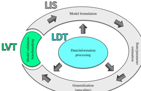
Figure 1. Schematic of the complete model–data fusion (MDF)
paradigm enabled by LDT, LIS, and LVT (modeled after Fig. 1 in Williams et al., 2009). LDT is the data preprocessing environment that feeds into the modeling and data assimilation environment of LIS and also LVT (the model evaluation and benchmarking system).
scale datasets, e.g., climate model reanalyses in high vary-ing terrain-based regions. Examples include the Modern-Era Retrospective analysis for Research and Applications (MERRA) Spatial Downscaling for Hydrology tool (MSDH; Sen Gupta and Tarboton, 2016), which uses the R statisti-cal software package (e.g., https://cran.r-project.org/, last ac-cess: 30 May 2018); TopoSCALE, v.1.0 (Fiddes and Gruber, 2014); and the eartH2Observe data portal, which provides a suite of Python scripts that downscale meteorological fields from the European Union’s eartH2Observe dataset (https: //github.com/earth2observe/downscaling-tools, last access: 18 January 2018). However, these script-based or software toolkits typically only serve a select set of different meteoro-logical forcing datasets.
LDT shares some commonality with these processing tools, but it is designed to be a more generic and comprehen-sive environment for supporting a wider range of data pro-cessing needs for the land and hydrological modeling com-munities. It provides the user with many data processing op-tions in how datasets are generated onto a common projec-tion and grid, reducing inconsistencies and errors, especially when combining different parameter datasets. LDT uniquely supports the handling of a suite of land remote-sensing mea-surements and preprocessing requirements for data assim-ilation environments. In addition to these key functionali-ties, LDT can generate certain model initial conditions (e.g., climatologically averaged state fields) for deterministic and ensemble model runs, a capability that is often needed in routine model simulations. Furthermore, the software is en-hanced with advanced techniques such as the development of data-driven models based on machine learning (ML) tech-niques and Bayesian merging for adaptive downscaling and bias-correction methods. LDT can handle input datasets in their “native” formats, performs consistency checks to ensure
reasonable values (e.g., no missing values), and provides the outputs using the conventions and formats compliant with community data standards. Most processed outputs are writ-ten to a standardized, descriptive format known as the Net-work Common Data Format (NetCDF; Unidata, 2015).
3 Software design of the LDT framework
As noted earlier, LDT is designed to encompass a broad set of functionalities that complement the modeling, data assimila-tion and evaluaassimila-tion environments of the LIS framework. To-gether, the LDT-LIS-LVT series conforms to the MDF con-cept (Raupach et al., 2005), where LDT supports the input data processing needs of the modeling system of LIS and LVT provides the evaluation procedures to help with revis-ing and improvrevis-ing any of the input and model formulations. Figure 1, modeled after the schematic outlined in Williams et al. (2009), highlights these end-to-end connections and capabilities in support of the MDF paradigm. LDT plays a central role in enabling this vision, by providing the data and information processing capabilities, which LIS and LVT use to enable an iterative process of model formulation, state and parameter estimation and refinement, generalization, and model validation and benchmarking.
LDT shares an object-oriented framework design with LIS, with a number of points of flexibility known as “plug-ins”. Specific implementations (such as soil parame-ter datasets or a surface meteorological forcing) are added to the framework through the plug-in interfaces. LDT uses the plug-in-based architecture to support the processing of dif-ferent types of observational datasets, ranging from in situ, satellite, and remotely sensed products to reanalysis prod-ucts. The LDT software structure is organized into three lay-ers: (1) the LDT core layer, (2) the “Abstractions” layer, and (3) the “Use case” layer. The latter represents the functional implementations of the Abstractions layer. Figure 2 outlines this structure and what is defined further in each layer. The “core” top layer executes the generic functions of time man-agement, defining the output fields, geospatial transforms, top-level handling of the different model parameters, and me-teorological dataset processing. The Abstractions layer en-ables “pluggable” interfaces with which to incorporate dif-ferent features, run modes, model datasets, and other func-tionalities. Also, a key aspect of the Abstractions layer is the ability to reuse the plug-ins to support additional features and expand LDT’s capabilities.
Frame-LDT core C o re st ru ct u re an d fe at u re s Time management Logging and diagnostic I/O management Configuration Geospatial transformation Ab st ra ct io ns Model parameters Us e ca se im p le m en ta ti o n kjkj
- Vegetation, soils - Land/hydrological model-specific - Irrigation/crop parameters - Topographic Data assimilation observations Meteorological forcing data processing Forcing downscaling features Grid domains kjkj
- SMAP soil moisture - SMOPS soil moisture - GRACE terrestrial water storage
kjkj
- GDAS forcing - NLDAS-2 forcing - CHIRPS precipitation - TRMM precipitation kjkj - Forcing climatology generation - Temporal downscaling feature kjkj - Equidistant (lat-long) - Polar-stereographic - Lambert conformal
Figure 2.Schematic of LDT’s main software architecture, showing the various core structures, abstraction layer, and use case
implementa-tions.
work (ESMF; Hill et al., 2004) library. ESMF is a library framework to support the building and coupling of earth system model components. ESMF provides several “off-the-shelf” infrastructure utilities such as clock/time manager and generic constructs for storing and exchanging data between various system components. LDT utilizes several ESMF fea-tures for passing information between the plug-in compo-nents and the core routines.
A number of libraries to enable the support for common earth science data formats are also utilized in LDT. They include the latest NetCDF, version 4 (NetCDF-4), Hierar-chical Data Format (HDF5; The HDF Group, 2015), HDF-EOS (or HDF-4), and the GRidded Binary or General Reg-ularly distributed Information in Binary form (GRIB) data formats, versions 1 and 2. Currently, the GRIB data for-mats are supported using the European Centre for Medium-Range Weather Forecasts (ECMWF)’s GRIB Application Programming Interface (GRIB-API) library (ECMWF, 2015) and will be replaced with the latest ECMWF’s ecCodes. Finally, LDT handles other data format libraries, including the Tagged Image File Format (TIFF) and the Band Inter-leaved by Line (BIL) format, both used mostly with remotely sensed data and widely supported in GIS software environ-ments and applications. TIFF formatted files are read-in us-ing the Geospatial Data Abstraction Library (GDAL; http: //www.gdal.org/, last access: 31 January 2018) translation li-brary, which is linked and invoked via the FortranGIS project libraries (https://github.com/dcesari/fortrangis, last access: 31 January 2018).
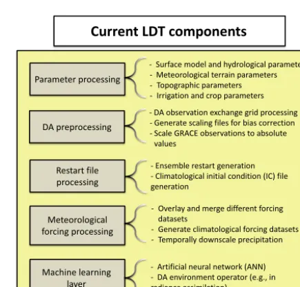
Current LDT components
Parameter processing DA preprocessing Restart file processing Meteorological forcing processing Machine learning layer
- Surface model and hydrological parameters - Meteorological terrain parameters - Topographic parameters - Irrigation and crop parameters - DA observation exchange grid processing - Generate scaling files for bias correction - Scale GRACE observations to absolute
values
- Ensemble restart generation - Climatological initial condition (IC) file generation
- Overlay and merge different forcing datasets
- Generate climatological forcing datasets - Temporally downscale precipitation
- Artificial neural network (ANN) - DA environment operator (e.g., in radiance assimilation)
Figure 3.Schematic depicting the current and different components
in LDT.
4 Capabilities and features of LDT
4.1 Model parameter processing support
For LSMs and hydrological models, the importance of pro-viding representative or “realistic” physical parameters has been shown in several studies (e.g., Sun and Bosilovich, 1996; Duan et al., 2006; Bounoua et al., 2006; Nearing et al., 2016). The key parameter types required for LSMs include (1) land cover/vegetation, (2) land/water mask, (3) soils, and (4) topography. Many land surface models contain tables of physical parameters that are indexed by spatial maps of pa-rameter types (e.g., roughness length indexed by land cover type or saturated hydraulic conductivity indexed by soil tex-ture class). Alternatively, physical parameters themselves may be specified on each model grid (e.g., snow-free albedo, green vegetation fraction). Adjunct models to LSMs include streamflow routing models and lake models. These models may be included with or separate from the LSM. Depending on their dimensionality and complexity, streamflow routing models require information about flow directions, drainage areas, slopes, roughness, and lengths of river reaches. Sim-ilarly, lake models require information about lake area and depth(s).
The first major parameter type of any land-based model is the vegetation or land cover (or use) classification map. Not capturing the correct land cover at different scales can lead to errors or impacts on other modeled processes, e.g., coupled feedbacks (Bounoua et al., 2006). Another feature in some LSMs is the concept of representing sub-grid het-erogeneity, also referred to as sub-grid “tiling”. Instead of considering the dominant land characteristics only, the sub-grid tiling approaches represent a sub-grid cell as a mosaic of a number of homogeneous elements, determined from the dis-tribution of land parameters within a grid cell (e.g., Avissar and Pielke, 1989; Koster and Suarez, 1992). Sub-grid tiling is aimed at better representing land surface model effects and feedback to coupled atmospheric models (e.g., Giorgi and Avissar, 1997; Essery et al., 2003; de Vrese et al., 2016). In addition to vegetation-based tiling, the effects of soil mois-ture distribution (e.g., Entekhabi and Eagleson, 1989) and elevation-based sub-grid variability (e.g., Leung and Ghan, 1995; Nijssen et al., 2001; Newman et al., 2014) on different water budget variables, like runoff and atmospheric response, have been investigated. LDT has been designed to support the representation of sub-grid tiling not only for vegetation but also for multidimensional combinations of properties, in-cluding soil types and topographic derivatives (e.g., eleva-tion, slope). Similar approaches have been developed for hy-drological response units to capture sub-grid heterogeneity for land model processes (Chaney et al., 2016).
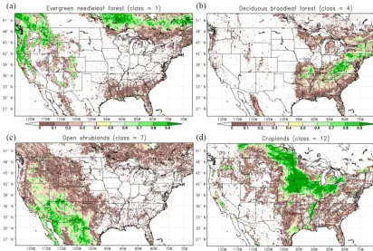
LDT uses the vegetation or land use map as a primary in-put parameter from which sub-grid heterogeneity can be sta-tistically represented and a corresponding land–water mask can also be derived. Figure 4 shows example vegetation tile frequency maps from four different vegetation classes (e.g., evergreen needle leaf, croplands) belonging to the Moderate
Resolution Imaging Spectroradiometer (MODIS) Interna-tional Geosphere-Biosphere Programme (IGBP) land cover classification map (Friedl et al., 2002). LDT can read in a moderately high-resolution vegetation map (e.g.,<1 km per grid cell) and generate the tiled frequency maps, as high-lighted in Fig. 4. In addition to land cover, LDT also repre-sents the sub-grid-scale distribution of soil types and topog-raphy datasets within a grid cell. The ability of LDT to rep-resent the distribution of fine-scale features of the underlying data for other land characteristics such as soils and topog-raphy allows a more flexible tiling representation, based on any of these features, or a combination of them. Land cover and land use map options in LDT include the U.S. Geologi-cal Survey (USGS) 24-class land cover (USGS GLCC), the University of Maryland (UMD) Advanced Very High Reso-lution Radiometer (AVHRR) land cover map (Hansen et al., 2000), and a few other dataset options, like Mosaic LSM veg-etation types (Koster and Suarez, 1996) and JULES (Dun-derdale et al., 1999).
Closely related to the vegetation type and land use pa-rameters described above is the “mask” field, which iden-tifies valid grid cells on which the model will run. Typically for a land surface or hydrological model, the mask discrimi-nates between land and open water points, assigning an index value, like 1, to the valid land points. In LDT, such a mask can be derived from the land classification map or read in and imposed. If imposed, LDT ensures that all processed pa-rameters are geographically co-registered and consistent with the input mask. A variety of options exist in LDT to ensure consistency between the masks and model parameters. These options include allowing the user to select neighboring grid cells to fill in a parameter value when the land mask indicates a valid land point but the parameter has a missing value. If no valid neighboring values are available (e.g., in the case of small islands), the user can then specify a universal value to fill in the missing data. In addition, LDT offers other param-eter processing features, such as upscaling (e.g., averaging) or downscaling techniques (e.g., bilinear interpolation) and different projections (e.g., equidistant geographic coordinate system, polar stereographic).
Figure 4.Vegetation distribution fraction of four different MODIS IGBP land cover classes (as produced by LDT): evergreen needleleaf
(a), deciduous broadleaf forest(b), open shrublands(c), and general cropland(d). Values greater than 0.9 indicate where more than 90 % of given grid cell (0.125◦grid cell resolution, in this example) is dominated by that vegetation type.
Figure 5.Comparison of the(a)STATSGO-FAO soil texture class
map (originally at 1 km resolution) versus the(b)ISRIC soil texture map (originally at 250 m resolution). Dominant texture classes are shown here at 10 km spatial resolution.
from the STATSGO-FAO and ISRIC soil texture maps, as processed through LDT.
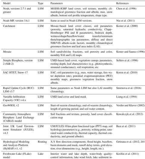
Currently, processing of the parameters for several land surface and hydrologic models is supported by LDT (and LIS), as summarized in Table 1. These models are the state-of-the art in representing the key processes of the terrestrial energy, water and carbon cycles as well as specialized
pro-cess representations of specific features of the land surface (e.g., lakes, urban). Some of the LSMs include Noah ver-sions 2.7.1 and later (Chen et al., 1996), Catchment LSM (Koster et al., 2000), JULES (Best et al., 2011), and several others. LDT also processes final inputs for the Hydrologi-cal Modeling and Analysis Platform (HyMAP) (Getirana et al., 2012, 2017), which is a hydrological routing scheme in LIS and collects and routes LSM-based total runoff through a network of catchments and tributaries to major river stems. Finally, LDT supports the processing of lake model param-eters, e.g., water depth for freshwater lake models such as FLake (Kirillin et al., 2011).
Table 1.LSMs and some of their parameters supported in LDT. Note that several LSMs use the land cover type and/or the soil texture type for each tile within LIS in combination with a lookup table to generate vegetation or soil parameters for that tile.
Model Type Parameters References
Noah, versions 2.7.1 and greater
LSM MODIS-IGBP land cover, soil texture, monthly
cli-matological greenness fraction and albedo, max. snow albedo, bottom soil profile temperature, slope type.
Chen et al. (1996)
Noah-MP, version 3.6.1 LSM Same as used in Noah LSM versions. Niu et al. (2011)
Catchment LSM Mosaic-based land cover classes, soil parameters
(porosity, saturated hydraulic conductivity, Clapp– Hornberger PSI and B parameters), bedrock depth,
wetness/shape/baseflow/water transfer/minimum
theta/topographic tau parameters, diffuse and direct NIR/VIS albedo-scale factors, monthly climatological greenness fraction and leaf area index (LAI).
Koster et al. (2000)
Mosaic LSM Soil sand/silt/clay fractions, soil porosity and color,
monthly SAI and LAI maps.
Koster and Saurez (1996)
Simple Biosphere, version 2 (SiB-2)
LSM UMD-based land cover, vegetation canopy parameters,
rooting depth, leaf characteristics (e.g., photosynthesis, stomatal conductance), soil respiration, etc.
Sellers et al. (1996)
SAC-HTET, Snow-17 LSM SAC: soil parameters (e.g., max. water storage, free
wa-ter depletion rate), potential evapotranspiration (PET) monthly maps, greenness vegetation fraction, snow albedo.
Koren et al. (2010)
Rapid Update Cycle (RUC) LSM v3.7
LSM Same parameters as Noah LSM but also LAI monthly
climatology.
Smirnova et al. (2016)
Variable Infiltration Capacity (VIC) v4.x
LSM UMD land cover and land mask Liang et al. (1994)
GeoWRSI, v2 LSM Start-of-season climatology, end-of-season climatology,
length of growing period, and soil water content.
Verdin and Klaver (2002)
Community Atmosphere Biosphere Land Exchange (CABLE) model
LSM Soil fractions and texture, porosity, land cover classifi-cation map
Kowalczyk et al. (2013)
Joint UK Land Environ-ment Simulator (JULES), v4.3
LSM UM/JULES 10 km plant functional type (PFT) map, soil
hydrology parameters (e.g., porosity, wilting point, satu-rated water conductivity, thermal capacity, thermal con-ductivity, and ground albedo).
Best et al. (2011)
Hydrological Modeling and Analysis Platform (HyMAP) v1, v2
Routing X,Y flow direction components, flood height, baseflow, basin domains and mask, runoff delay terms, grid eleva-tion, river dimensions (e.g., height, length, etc.).
Getirana et al. (2012, 2017)
Freshwater Lake (FLake) model
Lake Interior water and lake depth, water-body
quality-control information, lake wind fetch, lake sediment in-puts.
Kirillin et al. (2011)
To enable the topographical downscaling of meteorologi-cal fields for fine-smeteorologi-cale modeling, LDT processes elevation, slope, and aspect datasets. High-resolution precipitation cli-matology maps from the Parameter-elevation Relationships on Independent Slopes Model (PRISM; Daly et al., 1997) or from WorldClim (Fick and Hijmans, 2017) can be ingested
eleva-tion model (DEM) datasets (globally, 30 arcsec resolueleva-tion versions).
4.2 Generation of model initial conditions
Similar to model parameters, model initial conditions (ICs) are required by all LSMs to simulate land surface model states and fluxes (e.g., Cosgrove et al., 2004; Rodell et al., 2005). Climatologically averaged, state-based initial tions have been shown to provide more optimal initial condi-tions for LSM and hydrological model simulacondi-tions than other methods (Rodell et al., 2005). One example of improving the model initial conditions was shown in Xia et al. (2012), go-ing from a 1-year spin-up period, originally used in the North American LDAS, phase 1 (NLDAS-1), to two stages of run-ning several years and averaging selected dates (e.g., 1 Jan-uary) for NLDAS, phase 2 (NLDAS-2). Running for several years improved the initial conditions for the NLDAS-2 model simulations, whereas the 1-year NLDAS-1 spin-up produced “lingering effects” on the soil moisture fields. LDT offers a feature to generate such climatological initial conditions. The climatological initial conditions are generated by taking an average of the same date and time (e.g., 1 June, at 00:00 Z) over multiple years (e.g., 1982–2010).
LDT also provides the capability to produce an IC-based file to initialize an ensemble simulation, e.g., for a sea-sonal forecast ensemble, going from a single-member model “restart” file to a multi-member file, which we refer to as ensemble “disaggregation”. In addition, an option exists to calculate the ensemble average from a multi-member IC (or restart) file to form a single-member IC file, which we refer to as ensemble “aggregation”. These options can support ini-tializing data assimilation and forecast ensemble model sim-ulations.
4.3 Data processing support for land data assimilation
The use of observational data from satellites and other remote-sensing platforms is a growing area of research in the land/hydrological modeling community. The informa-tion from these observainforma-tional data sources is often used to improve the characterization of model states through data assimilation (DA; e.g., Reichle et al., 2002; Kumar et al., 2008c) and model parameters through inverse modeling tech-niques (e.g., Harrison et al., 2012). The computational sys-tems of DA and inverse modeling, built around the physical models, have their own data and processing requirements. Most DA systems are designed to address and improve the random errors in models and expect the input datasets to be generally unbiased relative to model estimates. A common approach in the land DA community to enable these “bias-blind” (Dee, 2005) systems is to rescale the observational data to be consistent with the model climatology, which is simply a multiyear average of model states. The development
of model and observational data climatologies to enable such reprocessing is supported within LDT.
For soil moisture data assimilation, a commonly used rescaling approach is called CDF matching where cumula-tive distribution functions (CDFs) are used to bias-correct and reduce differences in observation and model states (Re-ichle and Koster, 2004). This scaling approach matches the CDF of the observation to that of the model and corrects all moments (e.g., first and second) of the observation distribu-tion, regardless of its shape. To generate CDFs with LDT, the user must supply multiple years of model output and observational data for the a given variable. LDT then pro-duces model- and observation-based CDF data, separately, at each model grid point, which the DA system can use to per-form the rescaling. The user can select the granularity, tem-poral averaging period, and data count threshold to generate the CDF files. The CDFs can also be generated either based on lumped annually based values (“lumped”) or seasonally stratified CDF values (i.e., “monthly”). Kumar et al. (2015) demonstrated that the use of seasonal CDFs reduces the sta-tistical errors from CDF matching in soil moisture DA, com-pared to the use of lumped CDFs. Finally, LDT can account for spatial sampling by using neighboring pixels to increase the sampling density in the CDF calculations (e.g., when a data record period is short; based on Reichle and Koster, 2004) or by grouping CDFs by land cover or soil texture type. LDT supports several different satellite-based observa-tional data types that can be used for data assimilation in LIS. These satellite-based observations include a variety of soil moisture (SM) retrievals, terrestrial water storage (TWS), and snow depth (SNWD). Table 2 summarizes the various products available in LDT, which encapsulate most modern land remote-sensing measurements.
Table 2.Different DA remotely sensed observational or land surface model data types supported in LDT and LIS.
Dataset type Description Reference
LPRM AMSR-E SM The Land Parameter Retrieval Model (LPRM)’s Advanced
Microwave Scanning Radiometer-Earth Observing System (AMSR-E) soil moisture retrievals.
Owe et al. (2008)
WindSat SM WindSat passive microwave soil moisture Li et al. (2010)
TUW ASCAT SM ESA’s Advanced Scatterometer (ASCAT) soil moisture,
processed at Technische Universität Wien, Austria.
Bartalis et al. (2008)
SMOS SM ESA’s Soil Moisture Ocean Salinity (SMOS) dataset Kerr et al. (2001)
GCOM-W AMSR2 SM Global Change Observation Mission (GCOM) AMSR
ver-sion 2 soil moisture
Wentz et al. (2014)
SMAP SM NASA’s Soil Moisture Active-Passive (SMAP) level 3
products.
Entekhabi et al. (2014)
SMOPS SM NOAA’s Soil Moisture Operational Product Systems
(SMOPS) includes several soil moisture datasets: AMSR2, SMOS, and ASCAT
Liu et al. (2016)
ESA’s CCI ECV active+passive SM ESA’s Climate Change Initiative (CCI) essential climate
variable (ECV) blended active/passive microwave SM
Liu et al. (2011)
GRACE TWS NASA’s Gravity Recovery and Climate Experiment
(GRACE) TWS anomaly dataset
Tapley et al. (2004)
GCOMW AMSR2 SNWD AMSR2 passive microwave snow depth retrievals Wentz et al. (2014)
LIS LSM model output LIS land surface model output fields (e.g., soil moisture) Kumar et al. (2008a, b)
LDT also allows the definition of an “exchange grid” for DA, a domain that is used for the calculation of the obser-vation minus the model forecast estimates (called “innova-tions”). The use of the exchange grid allows improved con-sistency between observations and the simulated model fore-casts. The exchange grid information generated by LDT is then employed by the DA system in the calculation of data assimilation updates.
4.4 Processing support for meteorological forcing datasets
LSMs driven with higher spatial resolution and observational data have been shown to have improved land states and fluxes over coarser and model-only generated meteorological in-puts (e.g., Masson et al., 2003; Reichle et al., 2011). Higher-resolution forcing datasets can improve land model ICs, for example, in coupled atmospheric simulations (e.g., Kumar et al., 2008a; Case et al., 2008). LIS and LDT support a large variety of meteorological reanalysis, observational forcings, and seasonal climate forecast datasets. LDT supports a large suite of meteorological forcing data, and it can be used as a stand-alone tool to downscale spatially and temporally, to merge, and to quality control these different forcing datasets. The final meteorological fields are written to a single file in NetCDF-4 format.
At this time, LDT supports two basic ways of process-ing meteorological datasets. First, LDT can be used to spa-tially and temporally interpolate to downscale and merge (or “overlay”) different meteorological forcing datasets us-ing the “Metforcus-ing processus-ing” run mode option. A second option exists where the user can generate climatological forc-ing datasets to capture diurnal and seasonal cycles of longer-term forcing data records. This second feature works with a variety of meteorological datasets, including overlaying mul-tiple datasets, to generate a more comprehensive climatolog-ical forcing (available down to an hourly climatology). This climatology option can be used for different applications, in-cluding generating forcing used in forcing ensembles and cli-matology forecast capabilities.
4.5 Spatial and temporal forcing downscaling and disaggregation options
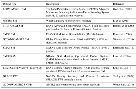
show-Figure 6.Examples of LDT-processed GRACE-based total TWS (in mm).(a)Plot of the LDT-processed TWS data for the southern African region for February, 2011 and(b)a time-series plot of the TWS data for years 2003–2015 and latitude of−21◦S and longitude of 24◦E.
ing improved meteorological and hydrological representa-tion at those scales. Also, temporal disaggregarepresenta-tion of coarser timescale forcing data (e.g., daily) has been shown to im-prove hydrological representation versus simply applying a uniform rate (e.g., over the day; Ryo et al., 2014). Such methods are also applied in the GLDAS (Rodell et al., 2004) and NLDAS (Cosgrove et al., 2003) forcing downscaling ap-proaches.
LDT offers some options for either spatially or temporally disaggregating forcing datasets. For temporal disaggrega-tion, forcing datasets that are at coarser timesteps, e.g., daily or greater, can be interpolated to a finer timestep (e.g., 3-hourly). For example, daily observed precipitation fields can be disaggregated using precipitation fields at finer timesteps, e.g., hourly fields from the MERRA, version 2 (MERRA-2), by applying weights from the MERRA-2 precipitation to create sub-daily precipitation from the daily product. This approach is based on Cosgrove et al. (2003), and it is pre-ferred for LSMs over other methods, e.g., simply distributing a daily precipitation product at the same rate (uniform) over each sub-daily (e.g., 3-hourly) timestep (e.g., Sen Gupta and Tarboton, 2016).
Current spatial downscaling techniques available from LDT, in conjunction with LIS, include using higher-resolution (e.g., 1 km), monthly precipitation climatology datasets, such as from the PRISM (Daly et al., 1997) or WorldClim (Fick and Hijmans, 2017) to spatially downscale coarser-scale precipitation data. Specifically, LDT calculates and stores the ratio of high-resolution precipitation climatol-ogy versus the same climatolclimatol-ogy aggregated at the coarser-scale resolution. These ratios reflect how spatial patterns of monthly precipitation change with respect to spatial resolu-tions and therefore provide a basis for spatially downscaling precipitation data when read into LIS. If the climatology of the precipitation data used to run LIS is also available, spa-tial downscaling can be performed in conjunction with bias correction. In this case, for example, LDT calculates the ratio of 1 km PRISM climatology to that of the coarser-scale
pre-cipitation used by LIS and stores the ratio (at the simulation resolution) in the LIS parameter file. LIS in turn reads the ratio and applies it to precipitation data each time when new forcing data are read. By definition, the output precipitation field from LIS will have the same climatology as PRISM in each calendar month, hence removing the bias of the coarser-scale precipitation climatology relative to that of the finer-scale precipitation climatology.
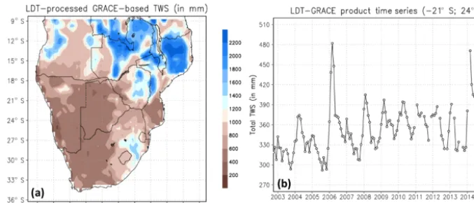
Figure 7.Examples of LDT-processed SRTM elevation parameter (in meters) at both(a)12.5 km and(c)1 km resolutions.(b)NLDAS-2 air temperature forcing field at its native 12.5 km resolution on 1 April 2005 (18:00 Z).(d)The 1 km resolution SRTM elevation field was then used to “topographically downscale” the NLDAS-2 air temperature (in units of K) using the lapse-rate correction approach for the finer-detailed 1 km air temperature field, as shown in plot(d).
4.6 The machine learning layer
Despite the huge advancements in modeling made possible by “physical” models, they have fundamental limitations in their ability to accurately portray the complex processes of the Earth system. For example, the significant human foot-print on the hydrological cycle has essentially led to a “re-plumbing” of the global hydrological cycle through activities such as agriculture and infrastructure development, leading to the recognition of a new geological epoch called the An-thropocene (Zalasiewicz et al., 2011). The accurate represen-tation of the replumbing is critical for understanding the sequences of human activity on water resources and its con-tribution to hydrological extremes. Due to the often subjec-tive nature of the human-engineered processes, the concep-tual physical models are limited in their ability to represent Anthropocene processes. On the other hand, large-scale ob-servations from satellites and remote-sensing platforms pro-vide a huge opportunity to represent them, which is only pos-sible if sophisticated data processing and data-driven models are available to fully exploit the information content of such measurements.
The availability of increased amounts of earth science data and the power of modern computers present an ideal
sce-nario for employing machine learning (ML) techniques for data-driven modeling and predictive analytics. ML-methods essentially develop nonlinear feature transformations learned from mapping a set of inputs to a set of outputs. More recent advancements in ML such as deep learning (Bengio, 2009), modeled after the human cognitive process, allow the model-ing of more complex relationships among the data and incre-mental learning. Generally, the data-driven ML models are a good alternative to the physical models when it is diffi-cult to build knowledge-driven simulation models in cases where the understanding of the underlying processes is lack-ing. With this recognition, LDT includes an ML layer de-signed to support a variety of ML algorithms and training models. The ML models developed from LDT are expected to augment the physical models and data assimilation envi-ronments.
Rainfall (LSM)
Snowfall (LSM)
Surface soil temperature (LSM) Green vegetation
fraction (LSM) Surface soil moisture (LSM)
In situ snow depth (GHCN)
Input layer
Hidden layer
Output layer
Spectral difference Tb18H - Tb36H (AMSR2) Spectral difference Tb18V - Tb36V (AMSR2)
Fractional snow cover (MODIS)
0 50 100 150 200 250 300 350
08/13 09/13 10/13 11/13 12/13 01/14 02/14 03/14 04/14 05/14 06/14 07/14
Snow depth (mm)
GHCN ANN prediction
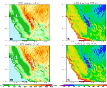
Figure 8. Example of the ML layer utilization in LDT. The top
panel shows the schematic of the ANN which ingests a suite of LSM-based and remote-sensing-based inputs for developing pre-dictions of snow depth. The bottom panel shows the performance of the trained network against in situ observations from the GHCN network.
the ANN. The trained network can then be used for generat-ing predictions with a new set of inputs.
The ML-based trained network models can be a useful op-erator within DA environments. Most satellite instruments detect radiances (electromagnetic energy over specific wave-lengths), and the conversion of these raw measurements to geophysical variable is not always trivial. The ML techniques can be used to develop models that translate between radi-ance measurements and related geophysical quantities. Such models can then be used in DA configurations, essentially al-lowing the direct use of raw satellite measurements in mod-eling.
An example of such a scenario is presented in Fig. 8. The input ML layer in LDT is used to ingest radiance mea-surements for the 18 and 36 GHz channels (both horizontal and vertical polarizations) from the AMSR2 instrument on the Global Change Observation Mission-Water (GCOM-W) satellite (Wentz et al., 2014). In addition, the input layer is presented with the fractional snow cover data from MODIS Terra instrument (MOD10A1) and the outputs from a LIS model simulation (variables including precipitation, green vegetation fraction, soil moisture, and soil temperature). The ANN within LDT is then trained against the daily snow depth measurements from the Global Historical Climate Network (GHCN) for a period of approximately 1 year (1 August 2012 to 31 July 2013). The training is conducted at a point location (Tierra Amarilla in New Mexico, 36.7◦E, 106.6◦W), where the snow evolution is often ephemeral, making an accurate
prediction difficult. The bottom panel of Fig. 8 shows the performance of the trained network, when used for prediction in the following year (1 August 2013 to 31 July 2014). The snow evolution is captured well by the ANN-based predic-tions. The specification of the input and output layers is user-defined and customizable. The ML layer in LDT can also be used for developing data-driven models both in a spatially distributed manner (where the training is done on a grid cell by grid cell basis) and on an aggregate basis (where a single trained model is developed using available inputs for all grid cells).
5 Summary and future capabilities
Land data assimilation systems (LDASs) require the integra-tion of high-quality observaintegra-tions with state-of-the-art land surface and hydrological models to acquire robust estimates of land surface conditions to meet the needs of applications involving weather and climate modeling, water resources management and modeling of hydrological extremes, among others. The synthesis of several types of model and obser-vation data across various spatial and temporal resolutions and extents is needed to support the development of flexi-ble LDAS configurations for conducting both research and application-oriented studies. To offer such a data fusion soft-ware framework, the Land surface Data Toolkit (LDT) has been developed with a large suite of capabilities including (1) parameter processing for a wide variety of models in-cluding land surface, hydrological, lake and streamflow mod-els; (2) the creation of initial conditions (e.g., climatological restarts) from model runs; (3) data assimilation preprocess-ing support; (4) meteorological forcpreprocess-ing data processpreprocess-ing for inputs to the models; and (5) data-driven models based on machine learning to assist the physical modeling and DA en-vironments. LDT provides a formal environment to handle the data-related needs within the model–data fusion concept, which is recognized to be essential for the systematic devel-opment and improvement of Earth system models.
LDT serves as the main preprocessor to the NASA Land Information System (LIS), which is an integrated framework designed for multi-model land surface model (LSM) and data assimilation (DA) integrations. LDT can also be used inde-pendently as an observational and model input processor for other land surface modeling systems. In addition, LDT offers a variety of user options to process model inputs, supports a variety of software libraries, has the ability to read in native (or original) dataset formats, and uses common data formats, like NetCDF-4.
the complex interactions of the terrestrial water, energy, and biogeochemical cycles. In addition, more detailed and fine-scale representations of the land surface (surface and subsur-face) also continue to grow, imposing an increased set of data requirements for their effective application at the scales of in-terest. A formal, extensive, and adaptive environment such as LDT is necessary to support these requirements. Similarly, the land DA applications and their complexity continue to grow with the increasing availability of remote-sensing ob-servations. Sophisticated data fusion models and processing algorithms are required to support the utilization of raw satel-lite measurements. With the increase in computing power and data science advancements, the machine learning and predictive analytics have become more commonplace in ar-eas involving e-commerce, social media, and health care. The data-rich Earth science arena is an ideal environment for de-ploying such data science enhancements and the machine learning (ML) layers in LDT will be continually updated to exploit such capabilities.
Future LDT capabilities will continue to include new parameter datasets (e.g., land cover, soil types), remotely sensed and in situ observations for DA preprocessing needs, projection grid types (e.g., Mercator projection), additional meteorological forcing datasets and downscaling techniques, and additional machine-learning methods. Parallel decompo-sition ability is also being developed and supported in LDT. Currently parallel capability is being tested with the meteo-rological forcing processing and downscaling and with some of the parameter processing features. New LSMs are cur-rently being implemented, including the Community Land Model (CLM; Oleson et al., 2010) and the latest versions of Noah and JULES LSMs. In addition, native parameter pro-cessing support is being considered for the Catchment and VIC LSMs, for HyMAP, and for other groundwater-based parameters. Finally, end-to-end data input processing for op-timization and parameter estimation along with uncertainty estimation techniques have been considered in future LDT versions, another component fulfilling the model–data fu-sion (MDF) paradigm with LIS and Land surface Verification Toolkit (LVT).
Code availability. The current version of LDT is release 7.2r ver-sion (6 May 2017 release), which is open-source and publicly avail-able from the main LIS website at https://lis.gsfc.nasa.gov/releases (last access: 22 August 2018; Kumar et al., 2006). The persistent identifier for this version is http://doi.org/10.5281/zenodo.1322613. The main LDT features described in this paper can be found with this release. Also, end-use test case examples are provided (https://lis.gsfc.nasa.gov/tests/ldt, last access: 14 March 2018; Ar-senault et al., 2018), and additional documentation, including the full user guide and tutorial type presentations, is located here: https://lis.gsfc.nasa.gov/documentation/ldt (last access: 14 March 2018; Arsenault et al., 2018). Future versions of the code will be made also available on GitHub (https://github.com/, last access: 25 July 2018; GitHub, 2018).
Author contributions. KRA and SVK designed and developed the main LDT software and led the writing of the paper and figure preparation. SVK is the lead architect of LDT and the Land Infor-mation System (LIS) software. JVG, SW, EK, DMM, HKB, AG, MN, BL, and JJ have developed and tested many components of the LDT software. JW and CDP-L have helped oversee and provided feedback on the development of LDT. KRA prepared the paper with contributions from all coauthors.
Competing interests. The authors declare that they have no conflict of interest.
Acknowledgements. We gratefully acknowledge the financial support from NASA Earth Science Technology Office (ESTO), the Air Force Life Cycle Management Center, NASA Applied Sciences Water Resources Program, NOAA’s Climate Program Office (MAPP program), NASA’s High Mountain Asia, SERVIR Applied Sciences Team and Terrestrial Hydrology, NASA’s Internal Research And Development (IRAD) program, and NASA’s Na-tional Climate Assessment (NCA) program, which all contributed to the development of LDT. Computing was supported by the resources at the NASA Center for Climate Simulation (NCCS). We also want to thank our user community for their invaluable feed-back in supporting LDT’s development and feature implementation.
Edited by: Jeffrey Neal
Reviewed by: two anonymous referees
References
Arsenault, K. R., Kumar, S., Geiger, J., Wang, S., Kemp,
E., Beaudoing, H., and Li, B: The Land surface
Data Toolkit (LDT) (Version version 7.2), Zenodo,
https://doi.org/10.5281/zenodo.1322613, 2017.
Avissar, R. and Pielke, R.: A parameterization of heterogeneous land surfaces for atmospheric numerical models and its impact on regional meteorology, Mon. Weather Rev., 117, 2113–2136, 1989.
Bartalis, Z., Naeimi, V., Hasenauer, S., and Wagner, W.: ASCAT Soil Moisture Product Handbook, Report No. ASCAT Soil Mois-ture Report Series, No. 15, 30 pp., 2008.
Bengio, Y.: Learning Deep Architectures for AI, Found. Trends in Mach. Learn., 2, 1–127, https://doi.org/10.1561/2200000006, 2009.
Best, M. J., Pryor, M., Clark, D. B., Rooney, G. G., Essery, R. L. H., Ménard, C. B., Edwards, J. M., Hendry, M. A., Porson, A., Gedney, N., Mercado, L. M., Sitch, S., Blyth, E., Boucher, O., Cox, P. M., Grimmond, C. S. B., and Harding, R. J.: The Joint UK Land Environment Simulator (JULES), model description – Part 1: Energy and water fluxes, Geosci. Model Dev., 4, 677–699, https://doi.org/10.5194/gmd-4-677-2011, 2011.
Case, J., Crosson, W., Kumar, S., Lapenta, W., and
Peters-Lidard, C.: Impacts of High-Resolution Land Surface
Initialization on Regional Sensible Weather Forecasts
from the WRF Model, J. Hydrometeorol., 9, 1249–1266, https://doi.org/10.1175/2008JHM990.1, 2008.
Chaney, N.W., Metcalfe, P., and Wood, E. F.: HydroBlocks: a field-scale resolving land surface model for application over continental extents, Hydrol. Process., 30, 3543–3559, https://doi.org/10.1002/hyp.10891, 2016.
Chen, F., Manning, K. W., LeMone, M. A., Trier, S. B., Alfieri, J.G., Roberts, R., Tewari, M., Niyogi, D., Horst, T. W., Oncley, S. P., Basara, J. B., and Blanken, P. D.: Description and Evaluation of the Characteristics of the NCAR High-Resolution Land Data Assimilation System, J. Appl. Meteor. Climatol., 46, 694–713, https://doi.org/10.1175/JAM2463.1, 2007.
Chen, F., Mitchell, K., Schaake, J., Xue, Y., Pan, H., Koren, V., Duan, Y., Ek, M., and Betts, A.: Modeling of land-surface evapo-ration by four schemes and comparison with FIFE observations, J. Geophys. Res., 101, 7251–7268, 1996.
Cosgrove, B. A., Lohmann, D., Mitchell, K. E., Houser, P. R., Wood, E. F., Schaake, J. C., Robock, A., Marshall, C., Sheffield, J., Duan, Q., Luo, L., Higgins, R. W., Pinker, R. T., Tarpley, J. D., and Meng, J.: Real-time and retrospec-tive forcing in the North American Land Data Assimila-tion System (NLDAS) project, J. Geophys. Res., 108, 8842, https://doi.org/10.1029/2002JD003118, 2003.
Cosgrove, B. A., Lohmann, D., Mitchell, K. E., Houser, P. R., Wood, E. F., Schaake, J. C., Robock, A., Sheffield, J., Duan, Q., Luo, L., Higgins, R. W., Pinker, R. T., Tarpley, J. D.: Land sur-face model spin-up behavior in the North American Land Data Assimilation System (NLDAS), J. Geophys. Res., 108, 8845, https://doi.org/10.1029/2002JD003316, 2004.
Daly, C., Taylor, G., and Gibson, W.: The PRISM approach to map-ping precipitation and temperature, 10th AMS Conf. on Applied Climatology, Reno, NV, 10–12, 1997.
Dee, D.: Bias and data assimilation, Q. J. Roy. Meteorol. Soc., 131, 3323–3343, 2005.
de Vrese, P., Schulz, J.-P., and Hagemann, S.: On the representation of heterogeneity in land-surface-atmosphere coupling, Bound.-Layer Meteorol., 160, 157–183, https://doi.org/10.1007/s10546-016-0133-1, 2016.
Duan, Q., Schaake, J., Andreassian, V., Franks, S., Goteti, G., Gupta, H.V., Gusev, Y. M., Habets, F., Hall, A., Hay, L., Hogue, T., Huang, M., Leavesley, G., Liang, X., Nasonova, O.N., Noilhan, J., Oudin, L., Sorooshian, S., Wagener, T., and Wood, E. F.: Model Parameter Estimation Experiment (MOPEX): An overview of science strategy and major results from the second and third workshops, J. Hydrol., 320, 3–17, https://doi.org/10.1016/j.jhydrol.2005.07.031, 2006.
Dunderdale, M., Muller, J. P., and Cox, P. M.: “Sensitivity of the Hadley Centre climate model to different earth observation and cartographically derived land surface data-sets”, in: The Contri-bution of POLDER and New Generation Spaceborne Sensors to Global Change Studies, 1–6, Meribel, France, 1999.
Entekhabi, D. and Eagleson, P.: Land surface
hydrol-ogy parameterization for atmospheric General
Circula-tion models including subgrid scale spatial variability,
J. Climate, 2, 816–831,
https://doi.org/10.1175/1520-0442(1989)002<0816:LSHPFA>2.0.CO;2, 1989.
Entekhabi, D., Yueh, S., O’Neill, P., et al.: SMAP Handbook, JPL Publication JPL 400-1567, Jet Propulsion Laboratory, Pasadena, California, 182 pp., 2014.
Esri, ArcGIS Desktop: Release 10.5, Redlands, CA: Environmental Systems Research Institute, 2016.
Essery, R. L. H., Best, M. J., Betts, R. A., and Cox, P. M.: Explicit representation of subgrid heterogeneity in a GCM land surface scheme, J. Hydrometeorol., 4, 530–543, 2003.
European Centre for Medium-Range Weather Forecasts (ECMWF): GRIB API version 1.10.0 and onwards, available at: https: //software.ecmwf.int/wiki/display/GRIB/Home (last access: 25 July 2018), 2015.
Fick, S. E. and Hijmans, S. E.: WorldClim 2: new 1-km spatial res-olution climate surfaces for global land areas, Int. J. Climatol., 37, 4302–4315, https://doi.org/10.1002/joc.5086, 2017. Fiddes, J. and Gruber, S.: TopoSCALE v.1.0: downscaling gridded
climate data in complex terrain, Geosci. Model Dev., 7, 387–405, https://doi.org/10.5194/gmd-7-387-2014, 2014.
Friedl, M. A., McIver, D. K., Hodges, J. C. F., Zhang, X. Y., Muchoney, D., Strahler, A. H., Woodcock, C. E., Gopal, S., Schneider, A., Cooper, A., Baccini, A., Gao, F., and Schaaf, C.: Global land cover mapping from MODIS: algo-rithms and early results, Remote Sens. Environ., 83, 287–302, https://doi.org/10.1016/S0034-4257(02)00078-0, 2002. Getirana, A. C., Boone, A., Yamazaki, D., Decharme, B., Papa,
F., and Mognard, N.: The Hydrological Modelling and Analy-sis Platform (HyMAP): Evaluation in the Amazon Basin, J. Hy-drometeorol., 13, 1641–1665, https://doi.org/10.1175/jhm-d-12-021.1, 2012.
Getirana, A., Peters-Lidard, C., Rodell, M., and Bates, P. D.: Trade-off between cost and accuracy in large-scale surface wa-ter dynamic modelling, Wawa-ter Resour. Res., 53, 4942–4955, https://doi.org/10.1002/2017WR020519, 2017.
Gesch, D. B., Verdin, K. L., and Greenlee, S. K.: New land surface digital elevation model covers the Earth, Eos Trans. AGU, 80, 69–70, https://doi.org/10.1029/99EO00050, 1999.
Giorgi, F. and Avissar, R.: Representation of heterogene-ity effects in Earth system modelling: Experience from
land surface modelling, Rev. Geophys., 35, 413–437,
https://doi.org/10.1029/97RG01754, 1997.
GitHub: available at: https://github.com, last access: 25 July 2018. Gochis, D. J., Yu, W., and Yates, D. N.: The WRF-Hydro model
technical description and user’s guide, version 2.0. NCAR Tech-nical Document, 120 pages, 2014, available at: WRF-Hydro 2.0 User Guide; WRF-Hydro Preprocesser Guide and Information: https://www.ral.ucar.edu/projects/wrf_hydro (last access: 25 July 2018), 2014.
Hansen, M., DeFries, R., Townshend, J. R. G., and Sohlberg, R.: Global land cover classification at 1km resolution using a decision tree classifier, Int. J. Remote Sens., 21, 1331–1365. https://doi.org/10.1080/014311600210209, 2000.
Harrison, K. W., Kumar, S. V, Peters-Lidard, C. D., and San-tanello, J. A.: Quantifying the change in soil moisture mod-elling uncertainty from remote sensing observations using Bayesian inference techniques, Water Resour. Res., 48, W11514, https://doi.org/10.1029/2012WR012337, 2012.
Gon-zalez, M. R.: SoilGrids1km – Global Soil Information Based on Automated Mapping, PLoS ONE, 9, e105992, https://doi.org/10.1371/journal.pone.0105992, 2014.
Hill, C., DeLuca, C., Balaji, V., Suarez, M., and da Silva, A.: The Architecture of the Earth System Modelling Framework, Com-put. Sci. Eng., 6, 18–28, 2004.
Jarvis, A., Reuter, H. I., Nelson, A., and Guevara, E.: Hole-filled SRTM for the globe Version 4, available from the CGIAR-CSI SRTM 90 m Database, available at: http://srtm.csi.cgiar.org (last access: 30 January 2018), 2008.
Kerr, Y. H., Waldteufel, P., Wigneron, J.-P., Martinuzzi, J.-M., Font, J., and Berger, M.: Soil Moisture Retrieval from Space: The Soil Moisture and Ocean Salinity (SMOS) Mission, IEEE T. Geosci. Remote Sens., 39, 1729–1735, 2001.
Kirillin, G., Hochschild, J., Mironov, D., Terzhevik, A.,
Golosov, S., and Nützmann, G.: Software, Data and
Modelling News: FLake-Global: Online lake model with worldwide coverage, Environ. Modell. Softw., 26, 683–684, https://doi.org/10.1016/j.envsoft.2010.12.004, 2011.
Koren, V., Smith, V., Cui, Z., Cosgrove, B., Werner, K., and Zamora, R.: Modification of Sacramento Moisture Accounting Heat Transfer Component (SAC-HT) for Enhanced Evapotran-spiration, NOAA Technical Report, NWS 53, U.S. Department of Commerce, NOAA National Weather Service, 2010. Koster, R. D. and Suarez, M. J.: Modelling the land surface
bound-ary in climate models as a composite of independent vegetation stands, J. Geophys. Res., 97, 2697–2715, 1992.
Koster, R. and Suarez, M.: Energy and Water Balance Calculations in the Mosaic LSM, NASA Tech. Memo. 104606, Vol. 9, 1996. Koster, R. D., Suarez, M. J., Ducharne, A., Stieglitz, M., and
Ku-mar, P.: A catchment-based approach to modelling land surface processes in a general circulation model: 1. Model structure, J. Geophys. Res., 105, 24809–24822, doi.10.1029/2000JD900327, 2000.
Koster, R., Sud, Y., Guo, Z., Dirmeyer, P., Bonan, G., Ole-son, K., Chan, E., Verseghy, D., Cox, P., Davies, H., Kowal-czyk, E., Gordon, C., Kanae, S., Lawrence, D., Liu, P., Mocko, D., Lu, C., Mitchell, K., Malyshev, S., McAvaney, B., Oki, T., Yamada, T., Pitman, A., Taylor, C., Vasic, R., and Xue, Y.: GLACE: The Global Land-Atmosphere Coupling Experiment. Part I: Overview, J. Hydrometeor., 7, 590–610, https://doi.org/10.1175/JHM510.1, 2006.
Kowalczyk, E., Stevens, L., Law, R., Dix, M., Wang, Y., Harman, I., Haynes, K., Srbinovsky, J., Pak, B., and Ziehn, T.: The land surface model component of ACCESS: Description and impact on the simulated surface climatology, Aust. Meteorol. Oceanogr. J., 663, 65–82, 2013.
Kumar, S., Peters-Lidard, C., Tian, T., Houser, P., Geiger, J., Olden, S., Lighty, L., Eastman, J., Doty, B., Dirmeyer, P., Adams, J., Mitchell, K., Wood, E., and Sheffield, J.: Land information sys-tem: An interoperable framework for high resolution land surface modelling, Environ. Model. Softw., 21, 1402–1415, 2006. Kumar, S., Peters-Lidard, C., Eastman, J. L., and Tao, W.-K.: An
in-tegrated high resolution hydrometeorological modelling testbed using LIS and WRF, Environ. Model. Softw., 23, 169–181, 2008a.
Kumar, S., Peters-Lidard, C., Tian, Y., Reichle, R. H., Alonge, C., Geiger, J., Eylander, J., and Houser, P.: An integrated hy-drologic modelling and data assimilation framework enabled by
the Land Information System (LIS), IEEE Comput., 41, 52–59, https://doi.org/10.1109/MC.2008.511, 2008b.
Kumar, S., Reichle, R., Peters-Lidard, C., Koster, R., Zhan, X., Crow, W., Eylander, J., and Houser, P.: A land surface data as-similation framework using the Land Information System: De-scription and Applications, Adv. Water Resour., 31, 1419–1432, https://doi.org/10.1016/j.advwatres.2008.01.013, 2008c. Kumar, S. V., Peters-Lidard, C. D., Santanello, J., Harrison, K.,
Liu, Y., and Shaw, M.: Land surface Verification Toolkit (LVT) – a generalized framework for land surface model evaluation, Geosci. Model Dev., 5, 869–886, https://doi.org/10.5194/gmd-5-869-2012, 2012.
Kumar, S. V., Peters-Lidard, C. D., Mocko, D., and Tian, Y.: Multi-scale Evaluation of the Improvements in Surface Snow Simula-tion through Terrain Adjustments to RadiaSimula-tion, J. Hydrometeor., 14, 220–232, https://doi.org/10.1175/JHM-D-12-046.1, 2013. Kumar, S. V., Peters-Lidard, C. D., Santanello, J. A., Reichle, R.
H., Draper, C. S., Koster, R. D., Nearing, G., and Jasinski, M. F.: Evaluating the utility of satellite soil moisture retrievals over irrigated areas and the ability of land data assimilation methods to correct for unmodeled processes, Hydrol. Earth Syst. Sci., 19, 4463–4478, https://doi.org/10.5194/hess-19-4463-2015, 2015. Kumar, S. V., Zaitchik, B. F., Peters-Lidard, C. D., Rodell, M.,
Re-ichle, R., Li, B., Jasinski, M., Mocko, D., Getirana, A., De Lan-noy, G., Cosh, M. H., Hain, C. R., Anderson, M., Arsenault, K. R., Xia, Y., and Ek, M.: Assimilation of Gridded GRACE Ter-restrial Water Storage Estimates in the North American Land Data Assimilation System, J. Hydrometeorol., 17, 1951–1972, https://doi.org/10.1175/JHM-D-15-0157.1, 2016.
Lehner, B., Verdin, K., and Jarvis, A.: New global hydrography de-rived from spaceborne elevation data. Eos, Transactions, AGU, 89, 93–94, 2008.
Leung, R. L. and Ghan, S. J.: A subgrid parameterization of oro-graphic precipitation, Theor. Appl. Climatol., 52, 95–118, 1995. Li, L., Gaiser, P. W., Gao, B.-C., Bevilacqua, R. M., Jack-son, T. J., Njoku, E. G., Rudiger, C., Calvet, J.-C., and Bindlish, R.: WindSat Global Soil Moisture Retrieval and Validation, IEEE T. Geosci. Remote Sens., 48, 2224–2241, https://doi.org/10.1109/TGRS.2009.2037749, 2010.
Liang, X., Lettenmaier, D. P., Wood, E. F., and Burges, S. J.: A simple hydrologically based model of land surface water and en-ergy fluxes for general circulation models, J. Geophys. Res., 99, 14415–14428, https://doi.org/10.1029/94JD00483, 1994. Liu, J., Zhan, X., Hain, C., Yin, J., Fang, L., Li, Z., and Zhao, L.:
”NOAA Soil Moisture Operational Product System (SMOPS) and its validations,” 2016 IEEE International Geoscience and Remote Sensing Symposium (IGARSS), Beijing, 3477–3480, https://doi.org/10.1109/IGARSS.2016.7729899, 2016.
Liu, Y. Y., Parinussa, R. M., Dorigo, W. A., De Jeu, R. A. M., Wagner, W., van Dijk, A. I. J. M., McCabe, M. F., and Evans, J. P.: Developing an improved soil moisture dataset by blending passive and active microwave satellite-based retrievals, Hydrol. Earth Syst. Sci., 15, 425–436, https://doi.org/10.5194/hess-15-425-2011, 2011.
Manabe, S.: Climate and the ocean circulation, Mon. Weather Rev., 97, 739–774, 1969.
G., Onof, C., Vrac, M., and Thiele-Eich, I.: Precipitation down-scaling under climate change: Recent developments to bridge the gap between dynamical models and the end user, Rev. Geophys., 48, RG3003, https://doi.org/10.1029/2009RG000314, 2010. Masson, V., Champeaux, J., Chauvin, F., Meriguet, C., and
Lacaze, R.: A Global Database of Land Surface Parame-ters at 1-km Resolution in Meteorological and Climate Mod-els, J. Climate, 16, 1261–1282, https://doi.org/10.1175/1520-0442(2003)16<1261:AGDOLS>2.0.CO;2, 2003.
McNally, A., Arsenault, K., Kumar, S. Shukla, S., Peterson, P., Wang, S., Funk, C., Peters-Lidard, C. D., and Verdin, J. P.: A land data assimilation system for sub-Saharan Africa food and water security applications, Sci. Data, 4, 170012, https://doi.org/10.1038/sdata.2017.12, 2017.
Miller, D. A. and White, R. A.: A conterminous
United States multilayer soil characteristics dataset
for regional climate and hydrology modelling,
Earth Interact., 2,
doi:https://doi.org/10.1175/1087-3562(1998)002<0001:ACUSMS>2.3.CO;2, 1998.
Mitchell, K. E., Lohmann, D., Houser, P. R., Wood, E. F., Schaake, J. C., Robock, A., Cosgrove, B. A., Sheffield, J., Duan, Q., Luo, L., Higgins, R. W., Pinker, R. T., Tarpley, J. D., Lettenmaier, D. P., Marshall, C. H., Entin, J. K., Pan, M., Shi, W., Koren, V., Meng, J., Ramsay, B. H., and Bailey, A. A.: The multi-institution North American Land Data Assimilation System (NLDAS): Uti-lizing multiple GCIP products and partners in a continental dis-tributed hydrological modelling system, J. Geophys. Res., 109, D07S90, https://doi.org/10.1029/2003JD003823, 2004. Monfreda, C., Ramankutty, N., and Foley, J. A.:
Farm-ing the planet: 2. Geographic distribution of crop ar-eas, yields, physiological types, and net primary production in the year 2000, Global Biogeochem. Cy., 22, GB1022, https://doi.org/10.1029/2007GB002947, 2008.
Nearing, G. S., Mocko, D. M., Peters-Lidard, C. D., Kumar, S. V., and Xia, Y.: Benchmarking NLDAS-2 Soil Moisture and Evapo-transpiration to Separate Uncertainty Contributions, J. Hydrom-eteor., 17, 745–759, https://doi.org/10.1175/JHM-D-15-0063.1, 2016.
Newman, A. J., Clark, M. P., Winstral, A., Marks, D., and Seyfried, M.: The use of similarity concepts to represent sub-grid variability in Land Surface Models: Case study in a snowmelt-dominated watershed, J. Hydrometeor., 15, 1717– 1738, https://doi.org/10.1175/JHM-D-13-038.1, 2014.
Nijssen, B., Schnur, R., and Lettenmaier, D. P.: Global Ret-rospective Estimation of Soil Moisture Using the Vari-able Infiltration Capacity Land Surface Model, 1980–93,
J. Climate, 14, 1790–1808,
https://doi.org/10.1175/1520-0442(2001)014<1790:GREOSM>2.0.CO;2, 2001.
Niu, G.-Y., Yang, Z.-L., Mitchell, K. E., Chen, F., Ek, M. B., Barlage, M., Kumar, A., Manning, K., Niyogi, D., Rosero, E., Tewari, M., and Xia, Y.: The commu-nity Noah land surface model with multiparameterization op-tions (Noah-MP): 1. Model description and evaluation with local-scale measurements, J. Geophys. Res., 116, D12109, https://doi.org/10.1029/2010JD015139, 2011.
Oleson, K. W., Lawrence, D. M., Bonan, G. B., Flanner, M. G., Kluzek, E., Lawrence, P. J., Levis, S., Swenson, S. C., and Thorn-ton P. E.: Technical Description of version 4.0 of the Community
Land Model (CLM), NCAR/TN-478+STR, National Center for
Atmospheric Research, Boulder, 2010.
Owe, M., de Jeu, R., and Holmes, T.: Multisensor historical clima-tology of satellite-derived global land surface moisture, J. Geo-phys. Res., 113, F01002, https://doi.org/10.1029/2007JF000769, 2008.
Ozdogan, M. and Gutman, G.: A new methodology to map irrigated areas using multi-temporal MODIS and ancillary data: An appli-cation example in the continental U.S., Remote Sens. Environ., 112, 3520–3537, 2008.
Ozdogan, M., Rodell, M., Beaudoing, H. K., and Toll,
D.: Simulating the effects of irrigation over the United
States in a Land Surface Model based on
satellite-derived agricultural data., J. Hydrometeorol., 11, 171–184, https://doi.org/10.1175/2009JHM1116.1, 2010.
Peters-Lidard, C. D., Houser, P. R., Tian, Y., Kumar, S. V., Geiger, J., Olden, S., Lighty, L., Doty, B., Dirmeyer, P., Adams, J., Mitchell, K., Wood, E. F., and Sheffield, J.: High-performance Earth system modeling with NASA/GSFC’s Land Information System, Innov. Syst. Softw. Eng., 3, 157–165, https://doi.org/10.1007/s11334-007-0028-x, 2007.
Rasmussen, R., Liu, C., Ikeda, K., Gochis, D., Yates, D., Chen, F., Tewari, M., Barlage, M., Dudhia, J., Yu, W., Miller, K., Grubisic, V., Thompson, G., and Gutmann, E.: High-resolution coupled climate runoff simulations of seasonal snowfall over Colorado: a process study of current and warmer climate, J. Climate, 24, 3015–3048, 2011.
Raupach, M., Rayner, P., Barrett, D., DeFries, R., Heimann, M., Ojima, D., Quegan, S., and Schmullius, C.: Model-data synthesis in terrestrial carbon observation: methods, data requirements and data uncertainty specifications, Global Change Biol., 11, 378– 397, 2005.
Reichle, R. H. and Koster, R. D.: Bias reduction in short records of satellite soil moisture, Geophys. Res. Lett., 31, L19501, https://doi.org/10.1029/2004GL020938, 2004.
Reichle, R. H., McLaughlin, D. B., and Entekhabi, D.: Hydrologic data assimilation with the ensemble Kalman filter, Mon. Weather Rev., 130, 103–114, 2002.
Reichle, R. H., Koster, R. D., De Lannoy, G. J., Forman, B. A., Liu, Q., Mahanama, S. P., and Touré, A.: Assessment and Enhancement of MERRA Land Surface Hydrology Estimates, J. Climate, 24, 6322–6338, https://doi.org/10.1175/JCLI-D-10-05033.1, 2011.
Reynolds, C. A., Jackson, T. J., and Rawls, W. J.: Estimating soil water-holding capacities by linking the Food and Agriculture Or-ganization Soil map of the world with global pedon databases and continuous pedotransfer functions, Water Resour. Res., 36, 3653–3662, https://doi.org/10.1029/2000WR900130, 2000. Rodell, M., Houser, P. R., Jambor, U., Gottschalck, J., Mitchell,
K., Meng, C-J., Arsenault, K., Cosgrove, B., Radakovich, J., Bosilovich, M., Entin, J. K., Walker, J. P., Lohmann, D., and Toll, D.: The Global Land Data Assimilation System, Bull. Am. Me-teorol. Soc., 85, 381–394, 2004.
Rodell, M., Houser, P., Berg, A., and Famiglietti, J.: Evaluation of 10 Methods for Initializing a Land Surface Model, J. Hydrome-teor., 6, 146–155, https://doi.org/10.1175/JHM414.1, 2005. Ryo, M., Saavedra Valeriano, O. C., Kanae, S., and Ngoc,