The NASA Eulerian Snow on Sea Ice Model (NESOSIM) v1.0: initial model development and analysis

https://doi.org/10.5194/gmd-11-4577-2018 © Author(s) 2018. This work is distributed under the Creative Commons Attribution 4.0 License.

The NASA Eulerian Snow on Sea Ice Model (NESOSIM) v1.0:

initial model development and analysis

Alek A. Petty1,2, Melinda Webster1, Linette Boisvert1,2, and Thorsten Markus1

1_{Cryospheric Sciences Laboratory, NASA Goddard Space Flight Center, Greenbelt, MD, USA} 2_{Earth System Science Interdisciplinary Center, University of Maryland, College Park, MD, USA}

Correspondence:Alek A. Petty ([email protected]) Received: 23 March 2018 – Discussion started: 7 May 2018

Revised: 14 October 2018 – Accepted: 18 October 2018 – Published: 16 November 2018

Abstract.The NASA Eulerian Snow On Sea Ice Model (NE-SOSIM) is a new, open-source snow budget model that is cur-rently configured to produce daily estimates of the depth and density of snow on sea ice across the Arctic Ocean through the accumulation season. NESOSIM has been developed in a three-dimensional Eulerian framework and includes two (vertical) snow layers and several simple parameterizations (accumulation, wind packing, advection–divergence, blow-ing snow lost to leads) to represent key sources and sinks of snow on sea ice. The model is forced with daily inputs of snowfall and near-surface winds (from reanalyses), sea ice concentration (from satellite passive microwave data) and sea ice drift (from satellite feature tracking) during the accu-mulation season (August through April). In this study, we present the NESOSIM formulation, calibration efforts, sen-sitivity studies and validation efforts across an Arctic Ocean domain (100 km horizontal resolution). The simulated snow depth and density are calibrated with in situ data collected on drifting ice stations during the 1980s. NESOSIM shows strong agreement with the in situ seasonal cycles of snow depth and density, and shows good (moderate) agreement with the regional snow depth (density) distributions. NE-SOSIM is run for a contemporary period (2000 to 2015), with the results showing strong sensitivity to the reanalysis-derived snowfall forcing data, with the Modern-Era Retro-spective analysis for Research and Applications (MERRA) and the Japanese Meteorological Agency 55-year reanalysis (JRA-55) forced snow depths generally higher than ERA-Interim, and the Arctic System Reanalysis (ASR) generally lower. We also generate and force NESOSIM with a consen-sus “median” daily snowfall dataset from these reanalyses. The results are compared against snow depth estimates

de-rived from NASA’s Operation IceBridge (OIB) snow radar data from 2009 to 2015, showing moderate–strong correla-tions and root mean squared errors of ∼10 cm depending on the OIB snow depth product analyzed, similar to the com-parisons between OIB snow depths and the commonly used modified Warren snow depth climatology. Potential improve-ments to this initial NESOSIM formulation are discussed in the hopes of improving the accuracy and reliability of these simulated snow depths and densities.

1 Introduction

Snow on sea ice is a crucial component of the polar cli-mate system. Its low thermal conductivity modulates sea ice growth through the cold winter months (e.g., Maykut and Untersteiner, 1971; Sturm et al., 2002), while its high surface albedo limits solar radiation absorption and thus inhibits sea ice melt in spring and summer (e.g., Warren, 1982; Grenfell and Perovich, 1984; Perovich et al., 2002). Conversely, fresh-water production from snowmelt facilitates melt pond forma-tion in spring–summer which lowers the surface albedo and promotes sea ice melt (Eicken et al., 2002, 2004). The ac-cumulation of snow on sea ice also modulates the freshwater flux into the ocean, a key component of the freshwater budget of the Arctic (e.g., Serreze et al., 2006).

sea ice above a local sea level, and estimates of snow depth to derive sea ice thickness, with snow depth being one of the primary sources of uncertainty for both laser and radar altimetry (e.g., Giles et al., 2007). Poor knowledge of snow density provides a further source of uncertainty through its influence on the ice freeboard and radar penetration into the snowpack (e.g., Giles et al., 2007; Kern et al., 2015).

Unfortunately, direct observations of snow depth and den-sity across the polar oceans are very limited, due to diffi-culties in remotely sensing this relatively thin (O(10 cm)) and heterogeneous medium and logistical challenges asso-ciated with in situ data collection. Passive microwave data have been used to estimate snow depth over first-year ice on a basin scale across both poles (e.g., Markus and Cav-alieri, 1998; Comiso et al., 2003; Maass et al., 2015), al-though these data are arguably more relevant for the first-year-dominated Antarctic sea ice pack and tend to underes-timate snow depth in deformed sea ice regimes (e.g., Worby et al., 2008; Brucker and Markus, 2013). Combinations of satellite and/or airborne sensors with variable snow penetra-tion depths are also being explored as a means of producing basin-scale snow depth estimates (e.g., Armitage and Rid-out, 2015; Guerreiro et al., 2016; Kwok and Markus, 2017), although this approach is still in its infancy and has limited temporal coverage. NASA’s Operation IceBridge has pro-vided airborne measurements of snow depth on sea ice since 2009 (Kurtz et al., 2013). However, the Arctic snow depth data collected are primarily limited to the western Arctic sea ice cover in spring (the spring 2017 campaign also included a flight over the eastern Arctic Ocean), while the Southern Ocean data have only been briefly explored to date (e.g., Kwok and Maksym, 2014). For the Arctic, a climatology of snow depth produced from Soviet drifting station data col-lected prior to 1991 (Warren et al., 1999) is still commonly used as a basin-scale snow depth product. The Soviet drift-ing station data also provide the only observationally based basin-scale assessment of snow density currently available. This snow climatology is expected to be outdated due to the rapid changes experienced in the Arctic climate system over the last few decades (Webster et al., 2014), although re-cent efforts have been made to modify this climatology based on ice type (halving the climatology over first-year ice, e.g., Laxon et al., 2013; Kwok and Cunningham, 2015).

Due to these observational limitations, the sea ice com-munity often utilizes simple models of snow depth forced by reanalyses (primarily snowfall data) (e.g., Maksym and Markus 2008; Kwok and Cunningham, 2008; Blanchard-Wrigglesworth et al., 2018). More sophisticated snow on sea ice models are available, such as SnowModel, a terrestrial snow model recently adapted for sea ice environments (Lis-ton et al., 2018), as well as the prognostic snow layer in-cluded in sea ice climate model components, such as the Los Alamos Sea Ice Model (CICE; Hunke and Lipscomb, 2010) and the Louvain-la-Neuve Sea Ice Model (LIM), which

have recently undergone various improvements to their snow physics (Holland et al., 2011; Lecomte et al., 2015).

In this study, we present a new model to derive snow depth (and density) across the Arctic Ocean. Our aim is to develop a model of physical and computational simplicity to allow for a detailed assessment of the sensitivity of snow depths to the various input forcing data needed to produce seasonal basin-scale snow depths. The spread in reanalysis-derived snowfall estimates over the Arctic Ocean is high (Boisvert et al., 2018), while the importance and uncertainty of other forcing data (e.g., ice concentration and drift) are still largely unknown. We also wanted a model that could be forced with observed ice concentration and drift to help accurately con-strain the seasonal sea ice cycle – a challenge for the more so-phisticated sea ice models described above. Our overall goal is that NESOSIM can be used to produce reliable basin-scale daily snow depth and density estimates needed for satellite altimetry calculations of sea ice thickness for both histor-ical analyses and near-real-time operations across the po-lar oceans. We thus expect the model to increase in com-plexity with future model developments, e.g., new parame-terizations or improvements to existing parameparame-terizations as needed. A secondary utility of the model will be the produc-tion of daily/monthly/seasonal snow depths from reanalysis data that can help guide climate modeling research efforts addressing the representation and importance of snow on sea ice in the global climate system.

In the following sections, we present and describe the model configuration/physics, the sensitivity of the model to the input forcing data (e.g., reanalyses snowfall, satellite-derived ice drifts) and model calibration/validation efforts. We focus this initial study solely on the Arctic; however, our plan is for the model to be applied and tested in a Southern Ocean framework in the near future. We conclude by look-ing ahead to potential improvements in the model physics and planned future activities related to our efforts to improve our understanding of snow on sea ice.

2 Model description

Snow accumulation Precipitation (snowfall)

Snowfall into the ocean

h_snew

h_sold

New fresh snow

Old compacted snow Wind packing

Wind blown snow lost to leads

Sea ice

Dynamics ρ_snew

ρ_sold

NESOSIM

Ocean

Winds

Ice drift

Figure 1.Schematic of the NASA Eulerian Snow On Sea Ice Model (NESOSIM) v1.0 presented in this study. The red (blue) text indicates

processes that result in a loss (gain) of snow. “Dynamics” indicates the combination of ice–snow advection and convergence–divergence which can cause either loss or gain of snow.

We decided on a Eulerian snow budget approach (as op-posed to a Lagrangian approach, e.g., Kwok and Cunning-ham, 2008) for a number of reasons: (i) it provides a frame-work flexible to the availability (or lack of) ice drift data, increasing the utility of the model in regions/time periods where ice drift data might be lacking; (ii) it provides a simple assessment of the spatial significance of the parameterized budget terms included in the model, including ice dynam-ics; and (iii) the parameterizations developed in this frame-work can be more easily transferred to other Eulerian sea ice models (e.g., the sea ice climate model component CICE) in-cluded in general circulation models (GCMs). The following subsections detail the model setup and various parameteriza-tions currently included in NESOSIM.

2.1 Model configuration

NESOSIM v1.0 includes two vertical layers on anx–y hor-izontal grid, with each horhor-izontal grid cell and snow layer featuring a prognostic snow depth and fixed snow density. This two-layer approach was taken to represent the strong differences in properties between dense snow, associated with wind slab, and fresh snow from recent snowfall, while keeping the model computationally efficient and the model physics easily trackable. As stated previously, our plan is that NESOSIM will be used for studying snow on sea ice across

the Arctic and Southern oceans; however, for this initial anal-ysis, we run the model on a 100 km×100 km polar stereo-graphic grid covering the Arctic Ocean and peripheral seas (model domain shown later in Fig. 5). This grid resolution was chosen due to considerations of computational efficiency and the horizontal resolutions of the various input data. The model is forced with daily data of snowfall and near-surface winds from reanalysis data, satellite passive microwave ice concentration and satellite-derived ice drifts.

At each daily time step, an effective snow depth within each grid cell is produced from our various snow budget terms (described in the following subsections) using a for-ward Euler method as

hs(t+1,0, x, y)=hs(t,0, x, y)+1haccs (t, x, y)

+1hdyns (t,0, x, y)+1hswp(t,0, x, y)+1hbss (t, x, y), (1) and

hs(t+1,1, x, y)=hs(t,1, x, y)+1hdyns (t,1, x, y)

+1hwps (t,1, x, y) , (2)

snowfall, and an “old” layer,ρ_so, which represents snow that has undergone wind compaction and snow grain metamor-phism (Colbeck, 1982; Sturm and Massom, 2017). These two fixed snow densities are justified in more detail in the follow-ing subsection. We track the evolution of an effective snow depth within each grid cell (the volume of snow per unit grid cell area) for simplicity. The actual snow depth over the ice fraction is calculated by dividing the effective grid-cell snow depth by the grid-cell ice concentration.

We also calculate a bulk snow density, which is the weighted average density across the two snow layers, as ρ_sb(t, x, y)=hs(t,0, x, y) ρsn+hs(t,1, x, y) ρso

.

hs(t,0, x, y)+hs(t,1, x, y)

. (3)

Note that the bulk snow density is masked if the respective ice concentration in the given grid cell is less than 15 %, or the effective snow depth is less than 2 cm. While the model tracks the snow budget terms for all grid cell ice concentra-tions, only grid cells with an ice concentration above 15 % are shown in the analysis, to prevent spurious interpretations in regions of near open water conditions.

Each annual model run is initialized in the middle of sum-mer (default of 15 August; rationale discussed in Sect. 2.5) and run until the following spring (1 May). This early sum-mer start time was chosen to include the significant snow-fall expected across the central Arctic through August (Ra-dionov et al., 1997; Warren et al., 1999; Boisvert et al., 2018) while also avoiding the periods of significant snowmelt in late spring to early summer/midsummer. We acknowledge that this end-of-August time period still likely includes sur-face melt events that are not captured/included in this model but are hoped to be addressed in future model developments. We also apply a variable initial snow depth (att=0) across our model domain, as discussed in Sect. 3.4. New ice that subsequently forms in a given grid cell is assumed to be snow free.

2.2 Snow accumulation

To accumulate snow on a given grid cell, the snowfall wa-ter equivalent from our reanalysis field is converted to snow depth using a representative snow density. Snow pit and den-sity data from the Surface Heat Budget of the Arctic Ocean (SHEBA) experiment and the Soviet drifting ice station data helped guide the parameterization of our seasonal snow den-sity evolution. Initially, snow accumulates into the new, fresh snow layer within a given grid cell as

1hacc_s (t, x, y)=Sf(t, xy) A (t, x, y) /ρsn, (4)

whereSf (in units of kg m−2) is the gridded daily snowfall

across the model domain andAis the gridded daily ice con-centration. The density of the new snow layer is fixed at ρ_sn=200 kg m−3. This value implicitly represents a combi-nation of cold, dry snowfall (∼150 kg m−3) and wet snowfall

(∼230 kg m−3) based on direct observations over Arctic sea ice (Radionov et al., 1997; Sturm et al., 2002).

Snow can be transferred from the new snow layer to the old snow layer depending on the strength of the near-surface wind forcing. The old snow layer is an implicit combina-tion of two layers that, on average, comprise the major-ity of the snowpack bulk mass: wind slab and depth hoar (Sturm et al., 2002; Sturm, 2009). The density of wind slab ranges between∼300 kg m−3and∼410 kg m−3on average (Colbeck, 1982; Radionov et al., 1997; Warren et al., 1999; Sturm et al., 2002), while depth hoar has an average density of ∼150–250 kg m−3 (Colbeck, 1982; Sturm et al., 2002). Based on SHEBA data, the Arctic snow cover consists of slightly more wind slab than depth hoar, comprising∼80 % of it collectively (Sturm et al., 2002). For this reason, we use a weighted average of the higher-end values of wind slab and depth hoar as the density value for the old snow layer,ρ_so. However, we note that the density and ratio of wind slab and depth hoar layers depend on several factors including the atmospheric conditions during precipitation events, sea ice surface roughness, snow depth and the internal snowpack temperature gradient (Sturm et al., 2002). We did experiment with alternative snow densities (e.g., the wider spread of 150 and 400 kg m−3) but found this provided worse correspon-dence with the seasonal snow density evolution compiled from in situ Soviet station data (introduced in Sect. 3.4).

When wind speeds are greater than 5 m s−1, the change in snow depth from wind packing between the two snow layers, respectively, is given as

1hwps (t,0, x, y)= −αTdhs(t,0, x, y)

for U (t, x, y) > ω, (5)

1hwps (t,1, x, y)= ρsn/ρso

αTdhs(t,0, x, y)

for U (t, x, y) > ω, (6)

whereUis the 10 m wind speed,ωis a wind action threshold for wind packing to occur (default of 5 m s−1),αis a wind-packing coefficient which determines the fraction of the new snow layer that is transferred into the old snow layer (default value of 5.8×10−7s−1), andTd is the number of seconds

in our daily time step (equivalent to 86 400 s). The second grid index in Eq. (2) (values of 0 and 1) represents the ver-tical snow layers. The wind action threshold of 5 m s−1was determined based on observational and modeling studies of blowing snow in the terrestrial Arctic and sea ice environ-ments (Pomeroy et al., 1997; Radionov et al., 1997; Sturm and Stuefer, 2013), while the wind-packing coefficient is a free, unconstrained parameter in the model.

2.3 Ice–snow dynamics

in Petty et al., 2018) to snow depth as 1hdyns (t, x, y)= −∇ ·

hs(t, x, y) ui(t, x, y)

, (7)

whereuiis the daily gridded ice motion. As in the ice

concen-tration budget studies discussed above, we can expand this into a divergence–convergence term and an advection term as

1hdiv_s (t, x, y)= −hs

t, x, y· ∇ui(t, x, y)

(8) and

1hadv_s (t, x, y)= −∇

hs(t, x, y)

·ui(t, x, y) , (9)

where 1hdiv_s is the change in effective snow depth from divergence–convergence, i.e., changes due to spatial gradi-ents in ice motion, and 1hadv_s is the change in snow depth from advection, i.e., changes due to spatial gradients in snow depth (assuming constant drift). Note that this parameter is applied to both “old” and “new” snow layers concurrently. 2.4 Blowing snow lost to leads

Snow within a grid cell can also be lost to leads/open wa-ter in the ice pack due to the impact of wind forcing, i.e., blowing snow lost to leads. This parameter is expected to be most significant in regions where high lead fractions, wind speeds and snowfall (e.g., the marginal ice zone in the North Atlantic sector of the Arctic) are expected to result in signifi-cant wind-blown snow lost to leads/open water (e.g., Leonard and Maksym, 2011). Note that we only apply this wind loss term to the new snow layer as we assume the “old” wind-packed snow layer is immune to the impact of wind forcing (e.g., Petrich et al., 2012; Trujillo et al., 2016). The blowing snow to leads term is calculated as

1hbs_s (t, x, y)= −βTdU (t, x, y)

hs(t,0, x, y)

1−A (t, x, y)for U (t, x, y) > ω, (10) where β is a blowing snow coefficient (default value of 2.9×10−7m−1). This is a free, unconstrained parameter in the model, with its default value chosen through our model calibration efforts.

We also keep track of snow that enters the ocean through snowfall into the open water fraction and blowing snow lost to leads, a quantity of relevance to those interested in the freshwater budgets of the polar oceans. This is given as S_foce(t, x, y)

=Sf(t, x, y)

1−A (t, x, y)

.

ρn_s−1hbs_s (t, x, y) . (11) For model testing, we also ran NESOSIM with differ-ent combinations of the model parameterizations discussed above. When we turn off the wind-packing parameteriza-tion, snow remains fixed in the “new” snow layer, despite

the strength of the wind forcing, so the model effectively becomes a one-layer model. To account for the low bias in snow density expected by constraining the snow density to the density of fresh, new snow, we forced this snow layer with the daily climatological snow density based on Warren et al. (1999), which we refer to asρ-W99.

3 Model forcing and calibration/validation data

In the following subsections, we describe the forcing data and calibration/validation data used in this study, includ-ing atmospheric forcinclud-ing data (snowfall and winds), satellite-derived ice motion, satellite-satellite-derived ice concentration, Soviet drifting station snow depths–densities (for model calibration) and Operation IceBridge snow depths (for model validation). 3.1 Atmospheric forcing

We use snowfall data provided by the European Centre for Medium-Range Weather Forecasts (ECMWF) ERA-Interim (ERA-I) reanalysis. ERA-I is a global reanalysis that utilizes a 4-D variational data assimilation scheme (Dee et al.,2011). We use the 12-hourly ERA-I snowfall data from 15 August 1980 to 1 May 1991 and 15 August 2000 to 1 May 2015. We use the 0.75◦×0.75◦horizontal resolution data, which are summed to produce daily snowfall estimates across the Arc-tic. ERA-I snowfall data have been used in previous stud-ies exploring snow accumulation over Arctic sea ice (e.g., Kwok and Cunningham, 2008; Blanchard-Wrigglesworth et al., 2018), while comparisons of reanalysis-derived precip-itation data with coastal weather stations suggest ERA-I is one of the better products available for Arctic studies (Ser-reze and Hurst, 2000; Lindsay et al., 2014). A more detailed comparison of snowfall–precipitation estimates over the Arc-tic Ocean has recently been carried out alongside this study (Boisvert et al., 2018), which we expect to build on in the future.

We explore the sensitivity of our results to the input snow-fall data by forcing the model with snowsnow-fall estimates pro-vided by three additional reanalysis-derived snowfall prod-ucts. Unfortunately, not all reanalyses provide direct esti-mates of snowfall (and rainfall) and instead provide just to-tal precipitation, e.g., the data from the widely used tional Centers for Environmental Prediction (NCEP) – Na-tional Center for Atmospheric Research (NCAR) reanaly-ses 1 and 2, so we focus our analysis on three other com-monly used reanalyses that provide direct estimates of snow-fall: the Japanese Meteorological Agency 55-year reanalysis (JRA-55); NASA’s Modern-Era Retrospective analysis for Research and Applications (MERRA); and the Arctic Sys-tem Reanalysis, version 1 (ASRv1), as described below and summarized in Table 2.

period 1958 to present (Kobayashi et al., 2015). JRA-55 was developed as an improvement to their previous 25-year re-analysis (JRA-25), which we do not include in this study. We use the daily JRA-55 snowfall data from 15 August 1980 to 1 May 1991 and 15 August 2000 to 1 May 2015. The data were obtained from the National Center for Atmospheric Re-search’s Research Data Archive at a horizontal resolution of 0.56◦×0.56◦ (∼60 km), downscaled from the original 1.25◦×1.25◦ Gaussian grid. The data are being produced on a near-real-time basis (2- to 6-month data latency).

MERRA.NASA’s MERRA is a global reanalysis that uti-lizes a 3-D variational data assimilation scheme within the Goddard Earth Observing System (GEOS-5) data assimi-lation system (Rienecker et al, 2011). We use the daily MERRA snowfall data from 15 August 1980 to 1 May 1991 and 15 August 2000 to 1 May 2015. The data are provided at a horizontal resolution of 0.5◦ _{(latitude) by 0.66}◦ (longi-tude). Note that an updated version of MERRA (MERRA-2) is also available, but is known to have a high precipitation bias compared to the other reanalyses (Boisvert et al., 2018), so we exclude this from our study.

ASRv1. ASRv1 is a regional reanalysis based on the Weather Research and Forecasting model (polar WRF) that utilizes a 3-D variational data assimilation scheme and is adapted for the polar regions (Hines and Bromwich, 2008). The ASRv1 data are only available from 2000 to 2012, so we use the daily snowfall data from 15 August 2000 to 1 May 2012, which is provided at a horizontal resolution of 30 km×30 km.

Considering the expected importance and uncertainty of the reanalysis-derived snowfall for deriving snow depth, we also produce a synthesized snowfall dataset by taking the me-dian snowfall across the gridded snowfall products for each daily grid cell (data referred to as MEDIAN-SF). We use the gridded ERA-I, JRA-55 and MERRA snowfall data, as these products all cover the longer-term (1980–2015) time period. NESOSIM also requires daily estimates of near-surface winds to drive the wind-packing and wind loss terms, which we take from the ERA-I reanalysis for all reanalysis model runs. Jakobson et al. (2012, Fig. 2) show that ERA-I winds had the lowest biases of several reanalysis-derived near-surface wind estimates compared to Tara drifting station data. We compute the magnitude of the winds from the 6-hourly u−v vectors before averaging to produce a daily (gridded) wind magnitude dataset.

We linearly interpolate all the daily snowfall (and ERA-I wind magnitude) estimates onto our 100 km×100 km po-lar stereographic model domain. Gridding scripts written in Python are included in the NESOSIM GitHub code repository (https://github.com/akpetty/NESOSIM, last up-date: 8 November 2018).

3.2 Satellite-derived ice motion data

We primarily make use of the daily Polar Pathfinder ice mo-tion data, version 3 (Tschudi et al., 2016) made available through the National Snow and Ice Data Center (the product is referred to herein as NSIDCv3). A daily ice motion vec-tor is calculated using a cross-correlation technique applied to sequential daily satellite images acquired by passive mi-crowave satellite sensors (i.e., a 1-day lag in parcel tracking) which are blended via optimal interpolation with estimates from the International Arctic Buoy Programme (IABP) and wind data from the NCEP/NCAR reanalysis. The data are available daily from October 1978 to February 2017 (at the time of writing) at a horizontal resolution of 25 km×25 km. In this study, we use the daily data from 15 August 1980 to 1 May 1991 and 15 August 2000 to 1 May 2015. We grid the daily ice motion data onto our 100 km model domain (us-ing linear interpolation) and smooth the data us(us-ing a simple Gaussian filter (as in Holland and Kimura, 2016 and Petty et al., 2018).

Recent studies have explored the uncertainty in satellite-derived ice motion data (Sumata et al., 2014) and errors in-troduced by the NSIDC interpolation methodology (Szanyi et al., 2016). We thus also explore the sensitivity of the model results to the input ice motion data by forcing the model with ice motion estimates provided by three additional satellite-derived ice motion products, as described below and summa-rized in Table 3.

Ocean and Sea Ice Satellite Application Facility (OSI SAF). The European Organization for the Exploitation of Meteorological Satellites (EUMETSAT) produce a number of low-resolution sea ice motion products from satellite pas-sive microwave sensors and scatterometry (Lavergne, 2010). Here, we use the merged ice motion product, which increases coverage and reliability over their single-sensor drift prod-ucts (Lavergne, 2010). The merged drift product uses a 2-day lag in ice parcel tracking and a continuous maximum cross-correlation (CMMC) method to optimize the drift product and has been available daily (October through April) since 2010 at a horizontal resolution of 62.5 km×62.5 km.

CERSAT.The Centre ERS d’Archivage et de Traitement (CERSAT), part of the Institut Français de Recherché pour l’Exploitation de la Mer (IFREMER), produces a number of ice motion datasets by merging various combinations of satellite passive microwave and scatterometry data (Girard-Ardhiun and Ezraty, 2012). Here, we use data produced from the merging of Advanced Scatterometer (ASCAT) and the Special Sensor Microwave Imager (SSM/I) data, which have been available daily (September to May) since 2007 at a hor-izontal resolution of 62.5 km×62.5 km. Note that CERSAT provides data using both a 3- and a 6-day lag in the tracking of ice displacement, but we use the 3-day lag data as this is closest to the 1-day lag used by the NSIDCv3 product.

Scanning Radiometer for Earth Observing System (AMSR-E) from January 2003 to September 2011 and the Ad-vanced Microwave Scanning Radiometer 2 (AMSR2) from July 2012 to December 2016 using a cross-correlation ap-proach (see Kimura et al., 2013 for more details). Wintertime (November–December, January–March) ice motion vectors are derived using the 36 GHz channel, while the summer-time drifts used in this study (August–October, April) are derived using the 18 GHz channel, to maximize the relia-bility and coverage of the data. The data are provided at a 60 km×60 km horizontal resolution.

We use data from these three additional products from 15 August 2010, 2012, 2013 and 2014 to 1 May of the subse-quent years, a period of coincident data coverage across the four drift products (including NSIDCv3). We linearly inter-polate all the daily drift datasets onto the 100 km×100 km polar stereographic model domain used in this study. As highlighted above, not all the products produce drift esti-mates in August, or even September, so for those products we assume no ice motion through this period. To investigate the importance of ice motion, we also run the model assuming no ice motion for the entire model simulation (NODRIFT), as discussed in more detail later.

3.3 Sea ice concentration

We use the daily Bootstrap sea ice concentration (SIC) data, version 3 (Comiso, 2000, updated 2017), which are produced from passive microwave brightness temperature estimates and made available through the NSIDC. We choose to pri-marily use the Bootstrap over, for example, NASA Team data (Cavalieri et al., 1996, updated 2017), another commonly used SIC dataset, as Bootstrap SIC data are less sensitive to surface melt, producing higher concentrations in general. We use the NASA Team data in a sensitivity study to explore the sensitivity of the model to this choice of sea ice concentra-tion data. Due to differences in satellite orbit and sensor char-acteristics, the SIC data feature a time-varying pole hole de-pending on the passive microwave sensor used. As we require consistent SIC data across the pole hole, we follow the ap-proach of Petty et al. (2018) and apply a mean SIC calculated in a 0.5◦halo around the variable pole hole to all grid cells within the pole hole. The data are provided at a 25 km×25 km resolution polar stereographic grid from 1978 to 2016, and we use the daily data from 15 August 1980 to 1 May 1991 and 15 August 2000 to 1 May 2015. We linearly interpolate the daily SIC data onto our 100 km×100 km model domain. Note that a gap in the passive microwave record exists from 3 December 1987 to 13 January 1988, so we do not run the model through the 1987–1988 winter period.

3.4 Soviet station data and initial conditions

We use in situ snow data collected on the former Soviet Union’s drifting ice stations for initial model calibration and

to help guide our choice of initial conditions (Radionov et al., 1997; Warren et al., 1999; Fetterer and Radionov, 2000). The drifting ice stations were in operation in 1937 and 1954– 1991, although in this study we use the field observations collected from 1980 to 1991 due to the temporal overlap with the model forcing data. During the drifting ice stations, snow depth data were collected every 10 days in 10 m intervals along a 500 or 1000 m survey line. Snow density measure-ments were made every∼100 m along the same survey lines, and atmospheric conditions were recorded at near-daily fre-quencies. Despite their limited spatial coverage, these data provide the most complete record of snow and atmospheric conditions to date over the Arctic sea ice pack.

Figure 2. (a)Warren climatology of August snow depth,(b, c)the initial conditions used in this study (broadly representing the snow depth as of 15 August) for 2012 and 2013, respectively, calculated using near-surface air temperature scaling.

Model calibration.For our model calibration, we use the raw snow depth and density data from the Soviet drifting sta-tions 25, 26, 30 and 31. The data represent the average of a given survey line. The majority of survey lines remained constant each time they were sampled, so the dataset is a near-continuous time series with a 10-day temporal reso-lution. Most survey lines were 1000 m in length, although in the earlier part of the historical record (e.g., before the 1980s), some ice stations had survey lines that were 500 m in length. Maps of the drifting stations are given in the sup-plementary information (Fig. S3 in the Supplement). Briefly, station 25 drifted from the central Arctic to the East Siberian Sea providing data from autumn 1981 to spring 1984, station 26 drifted around the north of the East Siberian Sea provid-ing data from autumn 1983 to sprprovid-ing 1984, station 30 drifted around the north of the East Siberian Sea providing data from autumn 1988 to winter 1991, and station 31 drifted around the Beaufort Sea providing data from winter 1989 to winter 1991. We use a simple nearest neighbor algorithm to match the data to the nearest model grid cell for the relevant day the drifting station data were collected.

3.5 NASA’s Operation IceBridge data

We compare our NESOSIM snow depth estimates with spring snow depths collected by NASA’s Operation Ice-Bridge (OIB) airborne mission. NASA’s OIB mission began collecting airborne observations of the polar regions in 2009, bridging the gap between NASA’s ICESat mission, which re-tired in 2009, and the future ICESat-2 mission scheduled for launch in the summer of 2018 (Markus et al., 2017). The OIB aircraft carry a suite of instruments designed to measure both land and sea ice, including their overlying snow cover. Here,

Sep Oct Nov Dec Jan Feb Mar Apr 0

10 20 30 40 50

Snow depth (cm)

r: 0.96

Soviet station NESOSIM

Sep Oct Nov Dec Jan Feb Mar Apr 180

200 220 240 260 280 300 320 340 360

S

no

w

d

en

si

ty

(

kg

m

−

3)

r: 0.97

0 10 20 30 40 50

SS snow depth (cm) 0

10 20 30 40 50

NESOSIM snow depth (cm)

r: 0.74 SN 25

SN 26 SN 30 SN 31

220 240 260 280 300 320 340 360 SS snow density (kg m−3₎

220 240 260 280 300 320 340 360

N

E

S

O

S

IM

s

no

w

d

en

si

ty

(

kg

m

−

3) r: 0.58

(a) (b)

(c) (d)

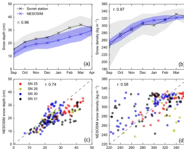
Figure 3.Comparison of NESOSIM snow depth(a, c)and snow density(b, d)data with drifting Soviet station data collected between 1981

and 1991. Panels(a, b)show the mean seasonal evolution of the snow depth and density for the model (blue) and Soviet station data (black), with the data binned into the different months the data were collected. The shaded area represents 1 standard deviation from the annual monthly mean. Panels(c, d)show scatter plots of all points for which there were temporal crossovers. Thervalues indicate the correlation coefficient, while the colors indicate the different stations that collected the data. The NESOSIM data are from the default/ERA-I model configuration.

4 Model calibration and analysis

We carried out model calibration over the period 15 August 1980–1 May 1991 due to the coincident Soviet station data available during this period. As noted previously, this ex-cludes the 1987–1988 winter season due to the lack of com-plete sea ice concentration data available during this period. As stated earlier, our initial calibration efforts involved man-ually tuning NESOSIM to improve the general fit with the mean seasonal snow depth–density cycles shown in the So-viet station data. Specifically, we included the temperature-scaled initial August snow depths and tuned both the wind-packing coefficient,α(Eq. 5), and blowing snow coefficient, β (Eq. 6). We decided against a more optimized calibra-tion effort due to limitacalibra-tions in the calibracalibra-tion data, i.e., its sparse availability in space–time and differences in spatial scales. We instead used the Soviet station data to guide our model choices to achieve a more realistic seasonal cycle in snow depth and density. We also decided against specific model configuration parameter tuning due to these limita-tions in the calibration data; however, this should be

con-sidered when analyzing the model performance, especially with regard to our validation efforts (i.e., more sophisticated and/or configuration-specific tuning could improve the com-parisons shown).

10 5 0 5 10

Snow depth difference (cm)

ρ-W99, NO WP, NO BSL, NO IC ρ-2lyr, WP, NO BSL, NO IC ρ-2lyr, WP, BSL, NO IC Default

(ρ-2lyr, WP, BSL, IC) Default, ω = 10 m s Default, α = 1.16e-6 Default, β = 5.8e-7

Sep Oct Nov Dec Jan Feb Mar Apr 100

80 60 40 20 0 20 40

S

no

w

d

en

si

ty

d

iff

er

en

ce

(

kg

m

−

3)

-1

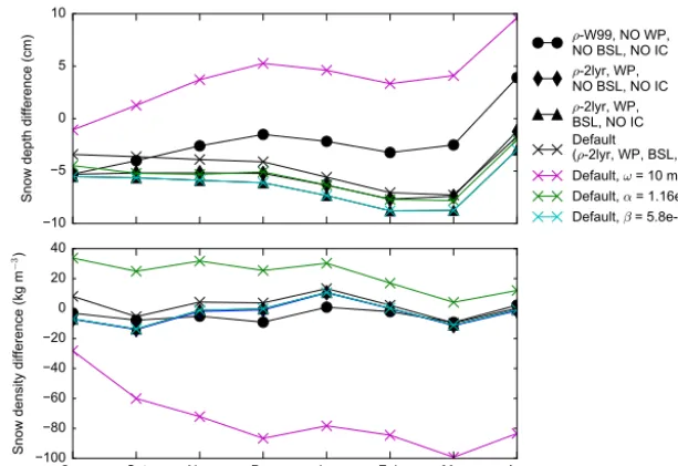
Figure 4.Differences between the mean (1980–1991) seasonal cycles in the drifting station data against various configurations of NESOSIM.

The different symbols represent different levels of model sophistication – ρ-W99: climatological Warren snow density, ρ-2lyr: default prognostic two-layer snow density, WP: wind-packing parameterization, BSL: blowing snow loss parameterization, IC: initial conditions. NO indicates that the parameterization/initial conditions have been turned off. The different colors then represent a doubling of individual model parameters, with all other settings fixed to the default settings (see Table 1). The black crosses and line represent the default/ERA-I results (as shown in Fig. 3).

density correlation strength is moderate (r=0.58), suggest-ing the model may be better captursuggest-ing regional variability in snow depth over snow density. It should be noted, how-ever, that snow density is highly variable in space and sub-ject to large measurement uncertainties when collected in situ (Sturm, 2009). In general, the moderate–high correlations and seasonal comparisons provide confidence in the utility of NESOSIM for estimating snow depths across the Arctic.

In Fig. 4, we highlight the sensitivity of NESOSIM to the chosen model configuration/sophistication, broadly rep-resenting the heuristic model tuning that was undertaken. First, we tested the results of NESOSIM with different com-binations of the various model parameterizations included. Note that, as discussed at the end of Sect. 2, when we turn off the wind-packing parameterization, the model essentially becomes a one-layer model, so we use a fixed Warren et al. (1999) seasonal snow density climatology (constant den-sity value across the Arctic). As this is based on the same drifting station data we compare our results to, it is perhaps unsurprising that this configuration provides a better match with the seasonal drifting station snow depth cycle, includ-ing deeper snow depths (and reduced low snow depth bias) from November to April. We chose to develop NESOSIM to allow for the production of snow depths that agree well with the old drifting station snow climatology but are able to also respond to the expected interannual variability and trends in Arctic climate over recent decades – hence the decision to develop and include a simple bulk density parameterization.

Including the blowing snow loss parameterization resulted in slightly lower snow depths (∼2 cm), but no significant change in snow density. This parameterization can impact the bulk density implicitly by reducing the amount of fresh snow contributing to the total snow depth–density. As the drifting station data are collected primarily within the central Arctic where ice concentrations are close to 100 %, it was expected that including blowing snow loss would not result in signifi-cant differences, as this parameterization is expected to pro-vide more of an impact in lower ice concentration regimes, where unfortunately in situ snow depth data are lacking. In-cluding the initial snow depths resulted in a small increase in snow depth and density, especially earlier in the seasonal cycle, as expected, reducing the low bias compared to the drifting station data. The seasonal correlations were similarly high across these model configurations, highlighting the pri-mary role of the model configuration choices in determining the general bias of the seasonal snow depth–density cycle.

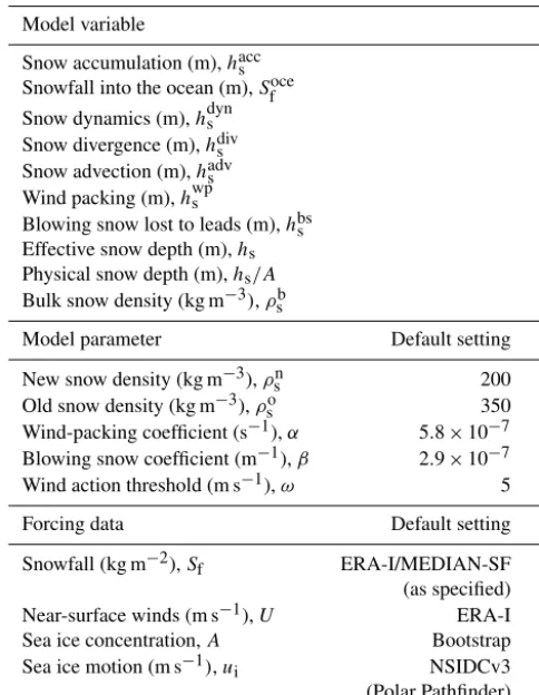
Table 1.Default model forcings and parameter settings used by NE-SOSIM.

Model variable

Snow accumulation (m),hacc_s

Snowfall into the ocean (m),S_foce

Snow dynamics (m),hdyns

Snow divergence (m),hdiv_s

Snow advection (m),hadv_s

Wind packing (m),hwps

Blowing snow lost to leads (m),hbs_s

Effective snow depth (m),hs

Physical snow depth (m),hs/A

Bulk snow density (kg m−3),ρ_sb

Model parameter Default setting New snow density (kg m−3),ρ_sn 200 Old snow density (kg m−3),ρ_so 350 Wind-packing coefficient (s−1),α 5.8×10−7 Blowing snow coefficient (m−1),β 2.9×10−7 Wind action threshold (m s−1),ω 5 Forcing data Default setting Snowfall (kg m−2),Sf ERA-I/MEDIAN-SF

(as specified) Near-surface winds (m s−1),U ERA-I Sea ice concentration,A Bootstrap Sea ice motion (m s−1),ui NSIDCv3

(Polar Pathfinder)

accumulates and remains in the fresher “new” snow layer for longer, significantly reducing the bulk snow density and in-creasing the seasonal snow depths. While this does produce snow depths that appear to agree better with the drifting sta-tion data, the low bias in the seasonal snow density suggests this is unphysical. Doubling the wind-packing coefficient,α (from 5.8×10−7to 1.16×10−6), has broadly the opposite effect, as expected, reducing the snow depths by increasing the transfer of snow from the fresher “new” snow layer to the denser “old” snow layer. Doubling the blowing snow loss coefficient, β (from 2.9×10−7to 5.8×10−7), has a negli-gible impact, again likely due to the location of the in situ data away from the lower concentration ice regimes where this process is more significant.

As stated earlier, the differences in spatial scales and data coverage (time and space) make interpreting these compar-isons/calibrations challenging. Specific model configurations may be required based on user demands, and our expecta-tion is for these calibraexpecta-tions to evolve as new calibraexpecta-tion data are made available and physical parameterizations intro-duced/updated. Note that we also compared the simulations of NESOSIM forced by the MERRA and JRA-55 snowfall data (Figs. S2 and S3). In general, the seasonal correlations with the drifting station data were similar to the ERA-I

re-sults, but the correlations of the raw data were slightly lower for JRA-55 (r=0.69 for snow depth andr=0.58 for snow density) and significantly lower for MERRA (r=0.44 for snow depth andr=0.57 for snow density). As discussed in Sect. 3, it is likely that specific model configuration tuning could improve these comparisons and the later validation ef-forts, but we decided against a more optimized calibration approach due to the limitations in the Soviet station data.

As discussed in Sect. 3.1, we also produced a synthesis snowfall dataset (MEDIAN-SF) using the median snowfall across the gridded ERA-I, JRA-55 and MERRA datasets. The MEDIAN-SF forced results are similar to the ERA-I re-sults (Fig. S4), in general, and show correlations similar to ERA-I and JRA-55 (r=0.68 for snow depth andr=0.58 for snow density). The MEDIAN-SF seasonal snow depths have a reduced low bias compared to the ERA-I results, al-though this difference is small. For the rest of this analysis, we choose to mainly focus on the MEDIAN-SF forced re-sults using the default configuration (Table 1) for simplicity. We provide a further assessment of the impact of the snowfall data in the following regional analysis and when we analyze the regional distributions across the more recent (2000–2015) time period.

5 Sensitivity studies and model validation

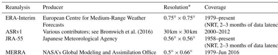
Table 2.Summary of the four different reanalysis datasets used in this study (data availability often subject to change/updates; information is given at the date of submission).

Reanalysis Producer Resolution∗ Coverage ERA-Interim European Centre for Medium-Range Weather 0.75◦×0.75◦ 1979–present

Forecasts (NRT, 2–3 months of data latency) ASRv1 Various contributors; see Bromwich et al. (2016) 30 km×30 km 2000–2012

JRA-55 Japanese Meteorological Agency 0.56◦×0.56◦ 1958–present

(NRT, 2–3 months of data latency) MERRA NASA’s Global Modeling and Assimilation Office 0.5◦×0.66◦ 1979–Jun 2016

∗_{Different resolutions available in some cases. NRT: near-real time.}

Table 3.Summary of the different ice motion datasets used in this study based on information obtained at the time of submission.

Product Resolution Daily lag Data source Coverage Availability NSIDCv3 25 km 1 day AVHRR, SMMR, SSM/I, Oct 1978–Feb 2017 Public

AMSR-E, IAPBs, NCEP-R1

OSI SAF 62.5 km 2 days AMSR-E, AMSR2, SSM/I, SSMIS, ASCAT∗ Dec 2009–present Public/NRT Kimura 60 km 1 day AMSR-E, AMSR2 Jan 2003–Sep 2011/ On request

Jan 2003–Sep 2011/

CERSAT 62.5 km 3 days ASCAT∗, SSM/I Jan 2007–present Public/NRT

∗_{These agencies produce drift datasets using different individual and/or combinations of satellite sensors not utilized in this study. NRT: near-real time.}

Figure 5.Map of the Arctic model domain and regions used in this

study: AO: Arctic Ocean, CA: central Arctic, EA: eastern Arctic, NA: North Atlantic; BS: Bering Sea, LS: Labrador Sea (peripheral seas also discussed in the paper).

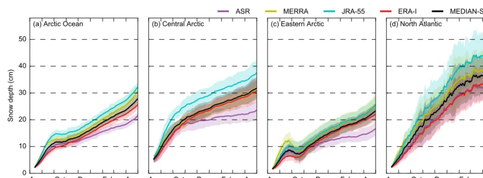
Figure 6 shows the seasonal snow depth and density evolu-tion across our four study regions for the 2000–2015 time pe-riod using the default/MEDIAN-SF configuration (Table 1). The AO and CA regions especially show strong initial in-creases in snow depth through fall (August to October) with the snow depth increasing at a slower rate from November to May, which is in good agreement with the W99 climatol-ogy. The EA and NA regions show a more uniform increase in snow depth from August to April. The NA region shows more daily snow depth variability, which was expected due to the strong ice drifts and the location of the NA storm track where passing cyclones can deposit large quantities of snow in a short period of time. It is also worth noting the small decline in snow depth through September–October in the EA region which is driven by reduced snowfall and snow densi-fication due to wind packing through this period. By 1 May, the mean snow depths (and interannual variability, calculated as 1 standard deviation of the annual values) are given as 27.8±1.9 cm (AO), 31.8±4.0 cm (CA), 23.2±2.9 cm (EA) and 42.5±8.1 cm (NA). The 1 May snow depth results are summarized in Table 4 to aid comparison with the snow depths produced in the following sensitivity studies.

Aug Oct Dec Feb Apr 0

10 20 30 40 50

Snow depth (cm)

(a) Arctic Ocean

Aug Oct Dec Feb Apr (b) Central Arctic

Aug Oct Dec Feb Apr (c) Eastern Arctic

Aug Oct Dec Feb Apr (d) North Atlantic

220 250 280 310 340

D

en

si

ty

(

kg

m

−

3)

Figure 6.Seasonal snow depth (black) and bulk density (green) evolution across the four study regions (shown in Fig. 5) initiated from

15 August 2000–2014 and run until 1 May of the following year using the MEDIAN-SF/parameter settings (Table 1). The thick lines show the mean values over this time period, while the shaded areas represent the interannual variability (1 standard deviation).

lower density) compared to the equal mix of old and new snow densities included in our initial conditions. The mean bulk snow densities as of 1 May are given as 309±2 kg m−3 (AO), 323±4 kg m−3_{(CA), 311±3 kg m}−3_{(EA) and 318±}

6 kg m−3_(NA).

5.1 Budget analysis

Here, we discuss the relative contributions to the seasonal snow depth evolution from the various snow budget terms currently included in NESOSIM. Results of the various NE-SOSIM budget terms and the total snow depth and bulk den-sity are shown in Fig. 7 across our four study regions for this 2000s time period. The black (green) lines and/or shading that represent the snow depth (bulk density) are the same as the results shown in Fig. 6.

Across the AO region, we see that accumulation is higher than snow depth, as expected (higher by∼30 cm by 1 May, around double the 1 May snow depth), with wind-packing (∼20 cm) and wind-blowing snow lost to leads (∼10 cm), providing significant reductions in snow depth. In the EA and CA regions especially, the blowing snow loss term is negligi-ble, while in the NA region it is more significant (contributes a sink of∼18 cm by 1 May). The NA region also shows a small (∼2 cm) increase (decrease) in snow depth driven by snow–ice divergence (ice–snow advection).

To further explore the different budget terms, we also show maps of the various budget terms as of 1 May over the same time period, as shown in Fig. 8. The maps highlight that many of these terms, especially the ice–snow dynam-ics (advection and convergence), exhibit high spatial vari-ability, which the regional means discussed previously mask. For example, the NA region shows a strong mix of posi-tive snow advection and convergence adjacent to the coast

of Svalbard (i.e., snow is advected into the region and is con-strained against the coastline) but an advection out of the re-gion further to the north as the ice either drifts down towards Svalbard/the Fram Strait or into the central Arctic.

The ice dynamic behavior around the pole is thought to be spurious considering interpolating issues across the pole hole in the NSIDCv3 drift product (Szanyi et al., 2016), which is one reason why we did not include this region in our regional analysis. In the following section, we assess the sensitivity of our results to the input ice motion dataset, which will pro-vide some further information as to the reliability of these dynamic budget terms.

As stated earlier, we hope to explore these decadal and re-gional differences more in future work. However, it is worth noting that the regional snow budget results and 1 May bud-get maps using the same default/MEDIAN-SF configuration but run for the 1980s time period were similar to the 2000s time period results (Figs. S4 and S5). The noteworthy dif-ferences in the budget terms include a less significant in-crease in blowing snow lost to leads in the CA region and less convergent driven snow depth increases in the new pe-riod, although accumulation and wind packing still dominate the budget terms for both periods. The NA results also do not show the advection-driven reduction in snow depth in March–April that was present in our 2000s results.

5.2 Reanalysis sensitivity study

re-Table 4.Mean snow depths as of 1 May across the four study regions (rows, regions given in Fig. 5) for NESOSIM using different forcings and time periods (columns). The numbers in brackets represent interannual variability and are calculated as 1 standard deviation of the annual values. The default NESOSIM configuration is MEDIAN-SF snowfall, ERA-I winds, NSIDCv3 ice motion and Bootstrap ice concentration.

NESOSIM configuration 1 May snow depth (cm)

Arctic Ocean Central Arctic Eastern Arctic North Atlantic (AO) (CA) (EA) (NA) Snowfall sensitivity results

2001–2015 (ASRv1) 21.4 (1.5) 23.5 (3.2) 16.6 (2.7) 37.4 (5.4) 2001–2015 (MERRA) 30.6 (2.6) 31.6 (3.1) 25.8 (3.6) 45.7 (9.0) 2001–2015 (JRA-55) 32.0 (1.9) 37.4 (4.7) 25.4 (3.3) 50.4 (9.5) 2001–2015 (ERA-I) 25.5 (1.7) 30.7 (4.1) 22.0 (2.5) 38.5 (7.3) 2001–2012 (MEDIAN-SF) 27.8 (1.9) 31.8 (4.0) 23.2 (2.9) 42.5 (8.1) Ice drift sensitivity results

2011–2015∗(MEDIAN-SF/NODRIFT) 27.3 (2.2) 32.4 (2.9) 24.8 (4.0) 38.7 (10.3) 2011–2015∗(MEDIAN-SF/OSI SAF) 26.3 (2.2) 32.9 (3.8) 23.4 (3.7) 38.9 (9.6) 2011–2015∗(MEDIAN-SF/Kimura) 25.7 (2.2) 32.9 (4.3) 21.2 (3.5) 38.9 (10.6) 2011–2015∗(MEDIAN-SF/CERSAT) 26.3 (2.2) 33.1 (3.9) 23.2 (3.6) 38.5 (10.0) 2011–2015∗(MEDIAN-SF/NSIDCv3) 26.7 (2.2) 32.4 (4.6) 22.9 (3.5) 39.9 (9.1) Ice concentration sensitivity results

2001–2015 (MEDIAN-SF/NASA Team) 23.4 (1.7) 28.0 (4.0) 20.3 (2.8) 35.4 (7.8)

∗_{Note that these 2011–2015 ice motion sensitivity runs exclude the 2012–2013 winter season due to the lack of Kimura drift data.}

Aug Oct Dec Feb Apr 30

0 30 60 90

Snow depth (cm)

(a) Arctic Ocean

Aug Oct Dec Feb Apr (b) Central Arctic

Aug Oct Dec Feb Apr (c) Eastern Arctic

Aug Oct Dec Feb Apr Snow accumulation

Blowing snow loss

Wind packing Convergence

Advection Physical snow depth

Bulk snow density

(d) North Atlantic

220 250 280 310 340

S

no

w

d

en

si

ty

(

kg

m

−

3)

Figure 7.Seasonal snow budget evolution across the four study regions (shown in Fig. 5), initiated from 15 August 2000 to 2014 and run

until 1 May of the following year using the default/MEDIAN-SF NESOSIM simulations. The thick lines show the mean daily regional values over this time period, while the shaded areas represent the interannual variability (1 standard deviation).

sults show significant differences in the seasonal snow depths across all regions (up to ∼10 cm across all regions). The rankings of snow depth between the different products are broadly consistent across the four regions, with JRA-55 and MERRA producing consistently higher snow depths (except

Figure 8.Snow budget terms as of 1 May, averaged over the 2001 to 2015 time period using the default/MEDIAN-SF NESOSIM simulations. The black lines show the four study regions used throughout this study. Panels(a)to(g)are integrals from the 15 August start date. Note the different color bar scales in panels(h)to(k).

all broadly similar, with JRA-55 significantly higher (by ∼5 cm from October onwards). It is thus expected that the MEDIAN-SF snowfall data will have excluded much of the high JRA-55 snowfall data (the benefits of using a median instead of a mean snowfall). Despite the NA region having the highest snow depths and interannual variability, the intra-reanalysis spread is similar to the other regions. The ASRv1 forced snow depths in the AO, CA and EA regions are

to this time period difference. The results further allude to the need for a consensus (e.g., median) snowfall dataset to force the model with the consideration of the large uncertainty in reanalysis-derived snowfall.

Figure 10 shows maps of the mean snow depths on 1 May over the same 2001–2015 time period, for the model sim-ulations forced by the MEDIAN-SF snowfall, then the dif-ferences from this MEDIAN-SF simulation using the four individual snowfall products.

The maps highlight the regional variability across the products but consistency in the MERRA/JRA-55 (ASR) high (low) difference compared to MEDIAN-SF. The JRA-55 and MERRA forced results both show significantly higher (10– 20 cm) snow depths through Bering Strait, the NA/Fram Strait region and the southern Labrador Sea. The ERA-I re-sults show slightly lower snow depths over most of the Arc-tic, small increases around the Canadian Arctic Archipelago and larger decreases in the Fram and Bering Strait region, driven by the larger differences in these regions in the MERRA/JRA-55 forcings. The magnitude of the precipita-tion events in Fram Strait are often large, but highly variable, due to the active storm track and the resulting difficulties of producing reliable precipitation rates during these events (Boisvert et al., 2018). As discussed earlier, it is challeng-ing to determine from this study any particular reanalysis-derived snowfall dataset that might be more appropriate (or an obvious outlier) for producing accurate snow depth esti-mates across the Arctic. However, the MEDIAN-SF forced results appear to provide a useful synthesis of the available snowfall data.

5.3 Ice motion sensitivity

We also explore the sensitivity of NESOSIM to the input satellite-derived ice motion data available during this period. Here, we show results from the default/MEDIAN-SF con-figuration forced by four different satellite-derived ice drift products: NSIDCv3, Kimura, CERSAT and OSI SAF, as de-scribed in Sect. 3.2. Due to limitations in the temporal cov-erage of the different drift datasets, the model is only run for 4 years initialized from 15 August 2011 to 2015 (exclud-ing 2012 initialized runs as Kimura data are not available due to gaps in the AMSR-E/AMSR2 record). The regional snow depth estimates from NESOSIM forced by these four ice drift products are shown in Fig. 11, with the 1 May results summarized in Table 4. In general, the ice drift sensitivity study shows a smaller spread in the mean snow depths across the different products (up to ∼3.5 cm), compared with the reanalysis sensitivity study (up to ∼13 cm). We also show results of NESOSIM forced with no ice drift (NODRIFT), which demonstrates that including ice drift appears not to be a crucial process for capturing the variability in snow depth at this regional scale; i.e., ice dynamics appear to be a clear second-order term compared to snowfall when analyzed at this regional scale.

The most obvious impact of ice drift is in the EA and NA regions. In the EA region, the inclusion of ice drift reduces the snow depth by 1.4–3.6 cm, with the magnitude depend-ing on the ice drift product chosen (the Kimura forced re-sults show the biggest decrease in this region). In the NA region, the inclusion of ice drift increases the snow depth by 3.8 to 5.3 cm (the NSIDCv3 forced results show the biggest increase in this region).

Figure 12 shows maps of the snow depths averaged on 1 May over the same 2011–2015 time period, for the model simulations assuming no drift (NODRIFT), then the differ-ences from this NODRIFT simulation using the various ice motion products. In general, the results show strong simi-larity in the spatial impacts of ice motion, including strong decreases in snow depth (up to∼10 cm) in the northeastern sector of the Arctic, and increases (up to∼10–20 cm) in the region directly north and west of Svalbard. There are clear differences between the different ice motion results, though, with the NSIDCv3 and Kimura forced results showing more of an impact on snow depth in the peripheral Arctic regions, e.g., strong decreases in the north and increases in the south Bering Strait, and strong increases in the Labrador Sea. This is thought to be driven primarily by the increased spatial coverage of these data compared to OSI SAF and CERSAT, which may be masking some of the ice motion data in these regions of low ice concentration and uncertain ice drift. The maps also highlight that, at more local scales, the ice dynamic contribution to snow depth variability could be significant. The data around the pole hole are also questionable in some of the products and may be related to interpolation issues across the pole hole. More specifically, the NSIDCv3 and OSI SAF forced simulations show increases in snow depth at the North Pole, which are not apparent in the CERSAT and Kimura simulations, suggesting this increase is likely spuri-ous.

In general, Figs. 11 and 12 suggest that the NSIDCv3 (Po-lar Pathfinder) forced simulations exhibit no obvious biases compared to the results using the other ice motion products, except for the issues of spurious snow depths within the pole hole and issues around the ice edge.

5.4 Ice concentration sensitivity

Aug Oct Dec Feb Apr 0

10 20 30 40 50

Snow depth (cm)

(a) Arctic Ocean

Aug Oct Dec Feb Apr

(b) Central Arctic

Aug Oct Dec Feb Apr

(c) Eastern Arctic

Aug Oct Dec Feb Apr

ASR MERRA JRA-55 ERA-I MEDIAN-SF

(d) North Atlantic

Figure 9.Seasonal snow depth evolution across the four study regions (shown in Fig. 5) initiated from 15 August 2000 to 2014 and run until

1 May of the following year, forced by five different reanalysis snowfall products. This figure also includes results using the ASRv1 forced simulations (which are limited to 15 August 2000 to 1 May 2012). The thick lines show the mean (daily) regional snow depths over this time period, while the shaded areas represent interannual variability (1 standard deviation). All model runs use the default forcings/parameter settings.

Figure 10.Simulated snow depths on 1 May (averaged over 1 May 2001 to 2015), using the MEDIAN-SF snowfall forcing(a)and then the

Figure 11.Seasonal snow depth evolution across the four study regions (shown in Fig. 5), initiated on 15 August 2010, 2012, 2013 and 2014, and run until 1 May of the following year, forced by four different ice motion datasets and assuming no ice motion (NODRIFT). The thick lines show the mean (daily) regional snow depths over this time period, while the shaded areas represent interannual variability (1 standard deviation). All model runs use the default/MEDIAN-SF parameter settings.

Figure 12.Modeled snow depth on 1 May (averaged over 1 May 2011, 2013, 2014 and 2015), assuming no ice motion (NODRIFT,a) and

Aug Oct Dec Feb Apr 0

10 20 30 40 50

Snow depth (cm)

(a) Arctic Ocean

Aug Oct Dec Feb Apr

(b) Central Arctic

Aug Oct Dec Feb Apr

(c) Eastern Arctic

Aug Oct Dec Feb Apr

Bootstrap NASA Team

(d) North Atlantic

Figure 13.Seasonal snow depth evolution across the four study regions (shown in Fig. 5), initiated from 15 August 2000 to 2014 and run

until 1 May of the following year, forced by the Bootstrap (magenta) and NASA Team (blue) ice concentration datasets. The thick lines show the mean (daily) regional snow depths over this time period, while the shaded areas represent interannual variability (1 standard deviation). All model runs use the default/MEDIAN-SF configuration.

This was somewhat expected given the known low bias in the NASA Team concentration data (e.g., Meier, 2005; Ivanova et al., 2015), reducing the concentration of sea ice for snow to accumulate on. More specifically, the Bootstrap data use daily variable tie points and are thus thought to im-prove the distinction between surface melt and open water. The lower concentrations also increase the blowing snow lost to leads term (as this is a function of the open water fraction). The snow budget terms using the NASA Team concentration data are shown in the Supplement (Fig. S7) to highlight this further, with all regions showing reduced snow accumula-tion and blowing snow lost to leads increased, and now sig-nificant, across all regions. Again, we believe the Bootstrap data better represent the seasonal ice conditions, although we appreciate that uncertainties still remain regarding the treat-ment of surface melt–melt ponds and their impact on snow accumulation/depth.

5.5 Validation with Operation IceBridge data

Here, we present and discuss comparisons of our NESOSIM snow depth estimates with NASA’s Operation IceBridge spring snow depth data from 2009 to 2015, as described in Sect. 3.5. We first show the basin-averaged results for the various OIB snow depth products each spring (from 2009 to 2015) and the coincident NESOSIM snow depth estimates, to assess how well NESOSIM captures the mean snow depth and expected interannual snow depth variability across this broad region of the Arctic. As discussed in Sect. 3.5, the OIB flights mainly cover the western Arctic sea ice pack, broadly within and to the west of the central Arctic domain used in our earlier regional analyses, although this does vary each year. Maps of the OIB snow depth retrievals across the dif-ferent products are given in Kwok et al. (2017).

2009 2010 2011 2012 2013 2014 2015

10 15 20 25 30 35 40 45

Snow depth (cm)

JRA55 MERRA ERAI MEDIAN

OIB-JPL OIB-GSFC OIB-SRLD

Figure 14.Comparisons of the annual mean snow depths from

NE-SOSIM (default configuration) forced with different reanalyses and the various Operation IceBridge (OIB) snow depth products. The blue (red) shading represents the annual mean spread across the dif-ferent NESOSIM results (OIB products). The markers are spread across the shaded areas to improve readability.

in terms of the mean snow depths and the broad pattern of interannual variability.

To assess how well the model captures regional snow depth variability, we show scatter plots in Fig. 15 of the NESOSIM/MEDIAN-SF snow depths and the three OIB snow depth products from 2009 to 2015 (the regressions for each year are given in Fig. S8). A summary of the correla-tion coefficients (r) and root mean squared errors (RMSEs) across the three OIB products and NESOSIM forced by the three individual (and median) reanalysis products for indi-vidual years and for all years of data is given in Table 5, with the regressions shown in Figs. S9–S11.

In general, the comparisons are highly variable and depend mainly on the chosen analysis year and the reanalysis snow-fall dataset, rather than the OIB product. The correlations between the OIB snow depth retrievals and the NESOSIM snow depths improve significantly in 2012 (r=0.63–0.75) compared to the proceeding years (r= −0.15–0.61). The im-proved correlations in 2012 onwards coincide with increases in the OIB flight coverage, which include more of the cen-tral Arctic and Beaufort and/or Chukchi seas, meaning the data better represent the regional variability in snow depths across the western Arctic. The strength of the correlations is highest in 2012 and 2013, while the RMSEs are lowest (<10 cm) between 2011 and 2013, especially in the ERA-I and MEDERA-IAN-SF forced results. The OERA-IB-SRLD RMSEs are generally lower than the RMSEs calculated with the other OIB products between 2010 and 2015, but significantly higher in 2009 when the signal-to-noise ratio of the earlier version of the snow radar used on OIB was higher (Kwok et al., 2017). The 2009 OIB snow depth results should thus be treated with caution.

The “all years” results in Table 5 provide a summary of the correlations using all the OIB snow depth retrievals from 2009 to 2015. The MERRA forced results produce signifi-cantly lower correlations to the OIB snow depths (r=0.37 to 0.43) compared to the other reanalyses, while the ERA-I forced results show the highest correlations (r=0.53 to 0.64) and lowest RMSEs (9–10 cm). The MEDIAN-SF re-sults show slightly lower correlations (r=0.47–0.58) and higher RMSEs (10–11 cm) compared to ERA-I. In general, however, the moderate-to-strong correlations give us confi-dence that NESOSIM is producing reasonable snow depth estimates across the western Arctic. The RMSEs of∼10 cm imply the expected level of accuracy in our NESOSIM snow depths, although these validations are hindered by uncer-tainty in the OIB snow depth retrievals (Kwok et al., 2017) and a lack of OIB retrievals in the eastern Arctic Ocean.

In the sensitivity studies presented earlier, we focused pri-marily on the MEDIAN-SF simulations, due in part to con-siderations of high snowfall variability in regions of high and uncertain precipitation, e.g., the North Atlantic sector. The OIB data lack coverage in this region, however, making it hard to assess if this synthesized forcing snowfall produces more accurate snow depths in these more challenging regions

of the Arctic. Data from the 2017 OIB flights into the eastern Arctic will hopefully provide some assessment of our NE-SOSIM snow depths in this region of the Arctic, however (the data were not available for this study but were made avail-able during the review phase of this paper). Our contempo-rary (2000–2015) NESOSIM results still lack validation of the simulated snow densities due to the lack of basin-scale density data available during this time period.

We can further assess the performance of NESOSIM by comparing these results with comparisons of OIB and the commonly used Warren snow depth climatology (Warren et al., 1999). As stated in the introduction, more recent uses of this climatology tend to apply a scaling factor (usually 50 %) to the snow depths over first-year ice. We follow the same approach here, using the EUMETSAT OSI SAF (www.osi-saf.org) ice-type product which is derived from a combination of passive microwave and scatterometry data at 10 km horizontal resolution (Breivik et al., 2012). We de-rive daily modified W99 snow depths (referred to herein as mW99) for the same 100 km bins used in Figs. 14 and 15 (where we have OIB data), with the comparisons shown in Fig. 16.

In general, these comparisons are similar, although in some cases the mW99 snow depths compare better with the OIB snow depths, depending on the product analyzed. Note that the bimodal nature of the mW99 data is due to the binary ice-type weighting scheme, which does significantly improve the comparison to the OIB data based on the RMSE and cor-relation coefficients (comparisons of unmodified W99 data are given in Fig. S12). The low RMSE values in the JPL-OIB comparison are driven by the very good agreement in the mean snow depth, while the GSFC and SRLD products tend to show a slight low bias, increasing the RMSE values. Figure 14 shows that the OIB-JPL product exhibits less in-terannual variability than the other products, which may pro-vide some explanation for the better correspondence with the W99 climatology. We also carried out OIB comparisons by delineating by ice type (first-year ice and multi-year ice) us-ing the same OSI SAF product discussed above. However, the results were mixed and were also strongly dependent on the OIB product analyzed. Such delineations are also hin-dered by the lower coverage of first-year ice in the OIB data, despite this becoming an increasingly dominant component of the Arctic sea ice pack. We thus chose to exclude this anal-ysis from our discussion for simplicity.

0 10 20 30 40 50 60 70 80 0

10 20 30 40 50 60 70 80

OIB snow depth (cm)

(a) SRLD

r: 0.58 RMSE: 10 cm

0 10 20 30 40 50 60 70 80 NESOSIM (MEDIAN-SF) snow depth (cm) 0

10 20 30 40 50 60 70 80 (b) JPL

r: 0.54 RMSE: 10 cm

0 10 20 30 40 50 60 70 80 0

10 20 30 40 50 60 70 80 (c) GSFC

r: 0.47 RMSE: 11 cm

Figure 15.Scatter plots of the three OIB snow depth products binned onto our 100 km model grid and coincident NESOSIM/MEDIAN-SF

snow depth estimates for all years of data from 2009 to 2015, including the correlation coefficient (r) and RMSE. The contours show the kernel density estimate of the distributions.

Table 5.Correlation coefficient (r, top rows) and root mean squared error (RMSE, bottom rows) from the correlations between the various

reanalysis-forced NESOSIM results and OIB-derived snow depths. The MEDIAN-SF scatter plots for all years of data are shown in Fig. 15, with other reanalysis-forced scatter plots given in the Supplement.

Year MEDIAN-SF ERA-I JRA-55 MERRA

SRLD JPL GSFC SRLD JPL GSFC SRLD JPL GSFC SRLD JPL GSFC

2009 0.27 0.17 0.30 0.37 0.24 0.36 0.32 0.19 0.36 0.18 0.12 0.21 17 cm 11 cm 12 cm 15 cm 10 cm 11 cm 21 cm 11 cm 12 cm 19 cm 11 cm 13 cm

2010 0.12 0.06 0.11 0.27 0.27 0.29 0.16 0.07 0.15 −0.06 −0.15 −0.08 12 cm 10 cm 11 cm 11 cm 9 cm 10 cm 16 cm 11 cm 14 cm 13 cm 12 cm 13 cm

2011 0.38 0.28 0.46 0.56 0.47 0.61 0.29 0.20 0.38 0.14 0.04 0.25 11 cm 8 cm 9 cm 10 cm 7 cm 8 cm 16 cm 9 cm 12 cm 10 cm 9 cm 10 cm

2012 0.73 0.70 0.73 0.75 0.72 0.75 0.72 0.67 0.72 0.67 0.63 0.66 8 cm 8 cm 9 cm 8 cm 8 cm 9 cm 12 cm 11 cm 10 cm 8 cm 9 cm 11 cm

2013 0.69 0.68 0.65 0.73 0.74 0.70 0.67 0.65 0.63 0.67 0.66 0.64 7 cm 13 cm 15 cm 7 cm 12 cm 14 cm 9 cm 10 cm 12 cm 7 cm 13 cm 15 cm

2014 0.68 0.63 0.63 0.74 0.70 0.68 0.64 0.58 0.60 0.53 0.48 0.52 10 cm 9 cm 11 cm 9 cm 9 cm 10 cm 12 cm 12 cm 15 cm 11 cm 10 cm 10 cm

2015 0.659 0.52 0.48 0.68 0.62 0.54 0.58 0.50 0.49 0.37 0.29 0.32 9 cm 10 cm 10 cm 8 cm 9 cm 9 cm 13 cm 11 cm 15 cm 10 cm 11 cm 10 cm

All years 0.58 0.54 0.47 0.64 0.62 0.53 0.57 0.53 0.47 0.43 0.41 0.37 10 cm 10 cm 11 cm 9 cm 9 cm 10 cm 14 cm 11 cm 13 cm 11 cm 11 cm 12 cm

6 Summary

In this study, we presented the newly developed NASA Eu-lerian Snow On Sea Ice Model (NESOSIM) version 1.0.