https://doi.org/10.5194/gmd-12-2419-2019 © Author(s) 2019. This work is distributed under the Creative Commons Attribution 4.0 License.
Simulating the effect of tillage practices with the global
ecosystem model LPJmL (version 5.0-tillage)
Femke Lutz1,2, Tobias Herzfeld1, Jens Heinke1, Susanne Rolinski1, Sibyll Schaphoff1, Werner von Bloh1, Jetse J. Stoorvogel2, and Christoph Müller1
1Potsdam Institute for Climate Impact Research (PIK), member of the Leibniz Association, P.O. Box 60 12 03, 14412 Potsdam, Germany
2Wageningen University, Soil Geography and Landscape Group, P.O. Box 47, 6700 AA Wageningen, the Netherlands Correspondence:Femke Lutz ([email protected])
Received: 12 October 2018 – Discussion started: 13 November 2018 Revised: 26 April 2019 – Accepted: 15 May 2019 – Published: 19 June 2019
Abstract.The effects of tillage on soil properties, crop pro-ductivity, and global greenhouse gas emissions have been discussed in the last decades. Global ecosystem models have limited capacity to simulate the various effects of tillage. With respect to the decomposition of soil organic matter, they either assume a constant increase due to tillage or they ignore the effects of tillage. Hence, they do not allow for analysing the effects of tillage and cannot evaluate, for ex-ample, reduced tillage or no tillage (referred to here as “no-till”) practises as mitigation practices for climate change. In this paper, we describe the implementation of tillage-related practices in the global ecosystem model LPJmL. The ex-tended model is evaluated against reported differences be-tween tillage and no-till management on several soil proper-ties. To this end, simulation results are compared with pub-lished meta-analyses on tillage effects. In general, the model is able to reproduce observed tillage effects on global, as well as regional, patterns of carbon and water fluxes. However, modelled N fluxes deviate from the literature values and need further study. The addition of the tillage module to LPJmL5 opens up opportunities to assess the impact of agricultural soil management practices under different scenarios with im-plications for agricultural productivity, carbon sequestration, greenhouse gas emissions, and other environmental indica-tors.
1 Introduction
More-over, other factors such as management practices (e.g. fertil-izer application and residue management) and climatic con-ditions have been shown to be important confounding factors (Abdalla et al., 2016; Oorts et al., 2007; van Kessel et al., 2013). For instance, Oorts et al. (2007) attributed the higher CO2emissions under no-till to higher soil moisture and de-composition of crop litter on top of the soil. Van Kessel et al. (2013) found that N2O emissions were smaller under no-till in dry climates and that the depth of fertilizer application was important. Finally, Abdalla et al. (2016) found that no-till effects on CO2 emissions are most effective in dryland soils.
In order to upscale this complexity and to study the role of tillage for global biogeochemical cycles, crop performance, and mitigation practices, the effects of tillage on soil prop-erties need to be represented in global ecosystem models. Although tillage is already implemented in other ecosystem models at different levels of complexity (Lutz et al., 2019; Maharjan et al., 2018), tillage practices are currently under-represented in global ecosystem models that are used for bio-geochemical assessments. In these, the effects of tillage are either ignored or represented by a simple scaling factor of decomposition rates. Global ecosystem models that ignore the effects of tillage include, for example, JULES (Best et al., 2011; Clark et al., 2011), the Community Land Model (Levis et al., 2014; Oleson et al., 2010) PROMET (Mauser and Bach, 2009), and the Dynamic Land Ecosystem Model (DLEM; Tian et al., 2010). The models in which the effects of tillage are represented as an increase in decomposition in-clude LPJ-GUESS (Olin et al., 2015; Pugh et al., 2015) and ORCHIDEE-STICS (Ciais et al., 2011).
The objective of this paper is to (1) extend the Lund Pots-dam Jena managed Land (LPJmL5) model (von Bloh et al., 2018) so that the effects of tillage on biophysical processes and global biogeochemistry can be represented and studied and (2) evaluate the extended model against data reported in meta-analyses by using a set of stylized management scenar-ios. This extended model version allows for quantifying the effects of different tillage practices on biogeochemical cy-cles, crop performance, and for assessing questions related to agricultural mitigation practices. Despite uncertainties in the formalization and parameterization of processes, the process-based representation allows for enhancing our understanding of the complex response patterns as individual effects and feedbacks can be isolated or disabled to understand their im-portance. To our knowledge, some crop models that have been used at the global scale, e.g. EPIC (Williams et al., 1983) and DSSAT (White et al., 2010), have similarly de-tailed representations of tillage practices but models used to study the global biogeochemistry (Friend et al., 2014) have no or only very coarse representations of tillage effects.
2 Tillage effects on soil processes
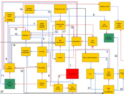
Tillage affects different soil properties and soil processes, re-sulting in a complex system with various feedbacks on pro-cesses related to soil water, temperature, carbon (C), and ni-trogen (N) (Fig. 1). The effect of tillage has to be imple-mented and analysed in conjunction with residue manage-ment as these managemanage-ment practices are often interrelated (Guérif et al., 2001; Strudley et al., 2008). The processes that were implemented into the model were chosen based on the importance of the process and its compatibility with the implementation of other processes within the model. Those processes are visualized in Fig. 1 with solid lines; processes that have been ignored in this implementation are visualized with dotted lines. To illustrate the complexity, we here de-scribe selected processes in the model affected by tillage and residue management, using the numbered lines in Fig. 1.
With tillage, surface litter is incorporated into the soil (1) and increases the soil organic matter (SOM) content of the tilled soil layer (2) (Guérif et al., 2001; White et al., 2010), while tillage also decreases the bulk density of this layer (3) (Green et al., 2003). An increase in SOM positively affects the porosity (4) and therefore the soil water holding capac-ity (whc) (5) (Minasny and McBratney, 2018). Tillage also affects the whc by increasing porosity (6) (Glab and Kulig, 2008). A change in whc affects several water-related pro-cesses through soil moisture (7). For instance, changes in soil moisture influence lateral runoff (8) and leaching (9) and affect infiltration. A wet (saturated) soil, for example, decreases infiltration (10), while infiltration can be enhanced if the soil is dry (Brady and Weil, 2008). Soil moisture af-fects primary production as it determines the amount of wa-ter which is available for the plants (11) and changes in plant productivity again determine the amount of residues left at the soil surface or to be incorporated into the soil (1) (feed-back not shown).
Figure 1.Flow chart diagram of feedback processes caused by tillage, which are considered (solid lines) and not considered (dashed lines) in this implementation in LPJmL5.0-tillage. Blue lines highlight positive feedbacks, red negative, and black are ambiguous feedbacks. The numbers in the figure indicate the processes described in Sect. 2.
influenced by changes in soil moisture (19) and soil temper-ature (20) (Brady and Weil, 2008). The rate of mineralization affects the amount of CO2emitted from soils (21) and the in-organic N content of the soil. Inin-organic N can then be taken up by plants (22), be lost as gaseous N (23), or transformed into other forms of N. The processes of nitrate (NO−3) leach-ing, nitrification, denitrification, mineralization of SOM, and immobilization of mineral N forms are explicitly represented in the model (von Bloh et al., 2018). The degree to which soil properties and processes are affected by tillage mainly depends on the tillage intensity, which is a combination of tillage efficiency and mixing efficiency (explained in detail in Sect. 3.2 and 3.5.2). Tillage has a direct effect on the bulk density of the tilled soil layer. The type of tillage determines the mixing efficiency, which affects the amount of incorpo-rating residues into the soil. Over time, soil properties recon-solidate after tillage, eventually returning to pre-tillage states. The speed of reconsolidation depends on soil texture and the kinetic energy of precipitation (Horton et al., 2016).
This implementation mainly focuses on two processes di-rectly affected by tillage: (1) the incorporation of surface lit-ter associated with tillage management and subsequent ef-fects (Fig. 1, path 1 and following paths) and (2) the decrease
in bulk density and the subsequent effects of changed soil water properties (Fig. 1, e.g. path 3 and following paths). In order to limit model complexity and associated uncer-tainty, tillage effects that are not directly compatible with the original model structure (such as subsoil compaction) or re-quire very high spatial resolution are not taken into account in this initial tillage implementation, despite acknowledging that these processes can be important.
3 Implementation of tillage routines into LPJmL 3.1 LPJmL model description
(e.g. mineralization of N and C). The water cycle is repre-sented by the processes of rain water interception, soil and lake evaporation, plant transpiration, soil infiltration, lateral and surface runoff, percolation, seepage, routing of discharge through rivers, storage in dams and reservoirs, and water ex-traction for irrigation and other consumptive uses.
In LPJmL5, all organic matter pools (vegetation, litter, and soil) are represented as C pools and the corresponding N pools with variable C:N ratios. Carbon, water, and N pools in vegetation and soils are updated daily as the result of com-puted processes (e.g. photosynthesis, autotrophic respiration, growth, transpiration, evaporation, infiltration, percolation, mineralization, nitrification, and leaching; see von Bloh et al., 2018, for the full description). Litter pools are repre-sented by the aboveground pool (e.g. crop residues, such as leaves and stubble) and the belowground pool (roots). The litter pools are subject to decomposition, after which the hu-mified products are transferred to the two SOM pools that have different decomposition rates (Fig. S1a in the Supple-ment). The fraction of litter which is harvested from the field can range between almost fully harvested or not harvested, when all litter is left on the field (90 %; Bondeau et al., 2007). In the soil, pools of inorganic, reactive N forms (NH+4, NO−3) are also considered. Each organic soil pool consists of C and N pools and the resulting C:N ratios are flexible. Soil C:N ratios are considerably smaller than those of plants as im-mobilization by microorganisms concentrates N in SOM. In LPJmL, a soil C:N ratio of 15 is targeted by immobilization for all soil types (von Bloh et al., 2018). The SOM pools in the soil consist of a fast pool with a turnover time of 30 years, and a slow pool with a 1000-year turnover time (Schaphoff et al., 2018a). Soils in LPJmL5 are represented by five hy-drologically active layers, each with a distinct layer thick-ness. The first soil layer, which is mostly affected by tillage, is 0.2 m thick. The following soil layers are 0.3, 0.5, 1.0, and 1.0 m thick, followed by a 10.0 m bedrock layer, which serves as a heat reservoir in the computation of soil temperatures (Schaphoff et al., 2013).
LPJmL5 has been evaluated extensively and demonstrated good skills in reproducing C, water, and N fluxes in both agri-cultural and natural vegetation on various scales (von Bloh et al., 2018; Schaphoff et al., 2018b).
3.2 Litter pools and decomposition
In order to address the residue management effects of tillage, the original aboveground litter pool is now separated into an incorporated litter pool (Clitter,inc) and a surface litter pool
(Clitter,surf) for carbon, and the corresponding pools (Nlitter,inc
and Nlitter,surf) for nitrogen (Fig. S1b in the Supplement). Crop residues not collected from the field are transferred to the surface litter pools. A fraction of residues from the sur-face litter pool are then partially or fully transferred to the incorporated litter pools, depending on the tillage practice:
Clitter,inc,t+1=Clitter,inc,t+Clitter,surf,t·TL for carbon and
Nlitter,inc,t+1=Nlitter,inc,t+Nlitter,surf,t·TL for nitrogen. (1)
The Clitter,surfand Nlitter,surfpools are reduced accordingly:
Clitter,surf,t+1=Clitter,surf,t·(1−TL),
Nlitter,surf,t+1=Nlitter,surf,t·(1−TL), (2)
where Clitter,incand Nlitter,incare the amounts of incorporated surface litter C and N, respectively, in grammes per square metre (g m−2) at a time stept(days). The parameter TL is the tillage efficiency, which determines the fraction of residues that is incorporated by tillage (0–1). To account for the ver-tical displacement of litter through bioturbation under natu-ral vegetation and under no-till conditions, we assume that 0.1897 % of the surface litter pool is transferred to the incor-porated litter pool per day (equivalent to an annual bioturba-tion rate of 50 %).
The litter pools are subject to decomposition. The decom-position of litter depends on the temperature and moisture of its surroundings. The decomposition of the incorporated lit-ter pools depends on soil moisture and temperature of the first soil layer (as described by von Bloh et al., 2018), whereas the decomposition of the surface litter pools depends on the litter’s moisture and temperature, which are approximated by the model. The decomposition rate of litter (rdecom in gC m−2d−1) is described by first-order kinetics, and is spe-cific for each plant functional type (PFT) following Sitch et al. (2003);
rdecom(PFT)=1−exp
− 1 τ10(PFT)
·g (Tsurf)·F (θ )
, (3) where τ10 is the mean residence time for litter and F (θ ) andg(Tsurf)are response functions of the decay rate to lit-ter moisture and litlit-ter temperature (Tsurf), respectively. The response function to litter moistureF (θ )is defined as: F (θ )=0.0402−5.005·θ3+4.269·θ2+0.7189·θ, (4) whereθ is the volume fraction of litter moisture which de-pends on the water holding capacity of the surface litter (whcsurf), the fraction of surface covered by litter (fsurf), the amount of water intercepted by the surface litter (Isurf) (Sect. 3.3.1), and lost through evaporationEsurf(Sect. 3.3.3). The temperature functiong (Tsurf)describes the influence of temperature of surface litter on decomposition (von Bloh et al., 2018):
g (Tsurf)=exp
308.56· 1 66.02−
1 (Tsurf+56.02)
, (5)
subject to the soil decomposition rules as described by von Bloh et al. (2018) and Schaphoff et al. (2018a). The min-eralized N (also 70 % of the decomposed litter) is added to the NH+4 pool of the first soil layer, where it is subjected to further transformations (von Bloh et al., 2018), whereas the humified organic N (30 % of the decomposed litter) is allo-cated to the different organic soil N pools in the same shares as the humified C. In order to maintain the desired C:N ratio of 15 within the soil (von Bloh et al., 2018), the mineralized N is subject to microbial immobilization, i.e. the transforma-tion of mineral N to organic N directly reverting some of the N mineralization in the soil.
The presence of surface litter influences the soil water fluxes and soil temperature of the soil (see Sect. 3.3 and 3.4), and therefore affects the decomposition of the soil carbon and nitrogen pools, including the transformations of mineral N forms. Nitrogen fluxes such as N2O from nitrification and denitrification, for instance, are partly driven by soil moisture (von Bloh et al., 2018):
FN2O,nitrification,l=K2·Kmax·F1(Tl)·F1 Wsat,l
·F (pH)·NH+4,lfor nitrification and
FN2O,denitrification,l=rmx2·F2 Wsat,l
·F2 Tl, Corg
·NO−3,lfor denitrification, (6) whereFN2O,nitrificationandFN2O,denitrificationare the N2O flux related to nitrification and denitrification, respectively, in gN m−2d−1in layerl.K2is the fraction of nitrified N lost as N2O (K2=0.02),Kmaxis the maximum nitrification rate of NH+4 (Kmax=0.1 d−1).F1(Tl)andF1 Wsat,lare response
functions of soil temperature and water saturation, respec-tively, that limit the nitrification rate.F (pH) is the function describing the response of nitrification rates to soil pH, and NH+4,l and NO−3,l the soil ammonium and nitrate concentra-tions in gN m−2, respectively. F2 Tl, Corg and F2 Wsat,l
are reactions for soil temperature, soil carbon, and water sat-uration andrmx2 is the fraction of denitrified N lost as N2O (11 %, the remainder is lost as N2). For a detailed description of the N-related processes implemented in LPJmL, we refer the reader to von Bloh et al. (2018).
3.3 Water fluxes 3.3.1 Litter interception
Precipitation and applied irrigation water in LPJmL5 is par-titioned into interception, transpiration, soil evaporation, soil moisture, and runoff (Jägermeyr et al., 2015). To account for the interception and evaporation of water by surface litter, the water can now also be captured by surface litter through litter interception (Isurf) and be lost through litter evaporation, sub-sequently infiltrates into the soil and/or forms surface runoff. Litter moisture (θ) is calculated in the following way: θt+1=min(whcsurf−θ(t ), Isurf·fsurf). (7)
fsurf is calculated by adapting the equation from Gre-gory (1982) that relates the amount of surface litter (dry mat-ter) per square metre (m2) to the fraction of soil covered:
fsurf=1−exp(−Am·OMlitter,surf), (8)
where OMlitter,surfis the total mass of dry matter surface lit-ter in grammes per square metre (g m−2) andAmis the area covered per mass of crop specific residue (m2g−1). The to-tal mass of surface litter is calculated assuming a fixed C to organic matter (OM) ratio of 2.38 (CFOM,litter), based on the assumption that 42 % of the organic matter is C, as suggested by Brady and Weil (2008):
OMlitter,surf=Clitter,surf·CFOM,litter, (9)
where Clitter,surfis the amount of C stored in the surface litter pool in grammes of carbon per square metre (gC m−2). We apply the average value of 0.004 forAmfrom Gregory (1982) to all materials, neglecting variations in surface litter for dif-ferent materials. whcsurf (mm) is the water holding capac-ity of the surface litter and is calculated by multiplying the litter mass with a conversion factor of 2×10⁻³mm kg−1
(OMlitter,surf) following Enrique et al. (1999).
3.3.2 Soil infiltration
The presence of surface litter enhances infiltration of pre-cipitation or irrigation water into the soil, as soil crusting is reduced and preferential pathways are affected (Ranaivo-son et al., 2017). In order to account for improved infiltration with the presence of surface litter, we follow the approach by Jägermeyr et al. (2016), which has been developed for imple-menting in situ water harvesting, e.g. by mulching in LPJmL. The infiltration rate (In in mm d−1) depends on the soil water content of the first layer and the infiltration parameterp;
In=prir· p s
1− Wa
Wsat,l=1−Wpwp,l=1
, (10)
where prir is the daily precipitation and applied irrigation water in millimetres,Wa the available soil water content in the first soil layer, and Wsat,l=1 andWpwp,l=1 the soil wa-ter contents at saturation and permanent wilting point of the first layer in millimetres. By defaultp=2, but four differ-ent levels are distinguished (p=3,4,5,6) by Jägermeyr et al. (2016), in order to account for increased infiltration based on the management intervention. To account for the effects of surface litter, we here scale the infiltration parameterp between 2 and 6, based on the fraction of surface litter cover (fsurf);
p=2·(1+fsurf·2). (11)
3.3.3 Litter and soil evaporation
Evaporation (Esurf in millimetres) from the surface litter cover (fsurf) is calculated in a similar manner as evaporation from the first soil layer (Schaphoff et al., 2018a). Evapora-tion depends on the vegetaEvapora-tion cover (fv), the radiation en-ergy for the vaporization of water (PET), and the water stored in the surface litter that is available to evaporate (ωsurf) rela-tive to whcsurf. Here,fsurfis also taken into account so that the fraction of soil uncovered is subject to soil evaporation as described in Schaphoff et al. (2018a);
Esurf=PET·α·max(1−fv,0.05)·ωsurf2 ·fsurf, (12)
ωsurf=θ/whcsurf, (13)
where PET is calculated based on the theory of equilibrium evapotranspiration (Jarvis and McNaughton, 1986) andαthe empirically derived Priestley–Taylor coefficient (α=1.32) (Priestley and Taylor, 1972).
The presence of litter at the soil surface reduces the evapo-ration from the soil (Esoil).Esoil(millimetres) corresponds to the soil evaporation as described in Schaphoff et al. (2018a), and depends on the available energy for vaporization of water and the available water in the upper 0.3 m of the soil (ωevap). However, with the implementation of tillage, the fraction of fsurf now also influences evaporation, i.e. greater soil cover (fsurf) results in a decrease inEsoil:
Esoil=PET·α·max(1−fv,0.05)·ω2·(1−fsurf), (14) where ω is calculated as the evaporation-available water (ωevap) relative to the water holding capacity in that layer (whcevap):
ω=min
1, ωevap whcevap
, (15)
whereωevapis all the water above wilting point of the upper 0.3 m (Schaphoff et al., 2018a).
3.4 Heat flux
The temperature of the surface litter is calculated as the av-erage of soil temperature of the previous day (t) of the first layer (Tsoil,l=1in◦C) and actual air temperature (Tair,t+1in ◦C), in the following way:
Tlitter,surf,t+1=0.5(Tair,t+1+Tsoil,l=1,t). (16)
Equation (16) is an approximate solution for the heat ex-change described by Schaphoff et al. (2013). The new up-per boundary condition (Tupper in◦C) is now calculated by the average ofTairandTsurfweighted byfsurf. With the new boundary condition, the cover of the soil with surface litter diminishes the heat exchange between soil and atmosphere;
Tupper=Tair·(1−fsurf)+Tsurf·fsurf. (17)
The remainder of the soil temperature computation remains unchanged from the description of Schaphoff et al. (2013).
3.5 Tillage effects on physical properties
3.5.1 Dynamic calculation of hydraulic properties Previous versions of the LPJmL model used static soil hy-draulic parameters as inputs, computed following the pe-dotransfer function (PTF) by Cosby et al. (1984). Different methods exist to calculate soil hydraulic properties from soil texture and SOM content for different points of the water re-tention curve (Balland et al., 2008; Saxton and Rawls, 2006; Wösten et al., 1999) or at continuous pressure levels (Van Genuchten, 1980; Vereecken et al., 2010). Extensive reviews of PTFs and their application in Earth system and soil mod-elling can be found in Van Looy et al. (2017) and Vereecken et al. (2016). We now introduce an approach following the PTF by Saxton and Rawls (2006), which was included in the model in order to dynamically simulate layer-specific hydraulic parameters that account for the amount of SOM in each layer, constituting an important mechanism of how hydraulic parameters are affected by tillage (Strudley et al., 2008).
As such, Saxton and Rawls (2006) define a PTF most suit-able for our needs and capsuit-able of calculating all the neces-sary soil water properties for our approach: The PTF allows for a dynamic effect of SOM on soil hydraulic properties, and is also capable of representing changes in bulk density after tillage and was developed from a large number of data points. With this implementation, soil hydraulic properties are now all updated daily. Following Saxton and Rawls (2006), soil water properties are calculated as
λpwp,l= −0.024·a+0.0487·Cl+0.006·SOMl+0.005
·Sa·SOMl−0.013·Cl·SOMl+0.068
·Sa·Cl+0.031, (18) Wpwp,l=1.14·λpwp,l−0.02, (19) λfc,l= −0.251·Sa+0.195·Cl+0.011·SOMl+0.006
·Sa·SOMl−0.027·Cl·SOMl+0.452
·Sa·Cl+0.299, (20) Wfc,l=1.238· λfc,l
2
+0.626·λfc,l−0.015, (21) λsat,l=0.278·Sa+0.034·Cl+0.022·SOMl−0.018
·Sa·SOMl−0.027·Cl·SOMl−0.584
·Sa·Cl+0.078, (22) Wsat,l=Wfc,l+1.636·λsat,l−0.097·Sa−0.064, (23)
BDsoil,l=(1−Wsat,l)·MD. (24)
SOMl is the soil organic matter content in weight percent
(wt %) of layerl;Wpwp,l is the moisture content at the
per-manent wilting point;Wfc,l is moisture contents at field
ca-pacity;Wsat,l is the moisture contents at saturation;λpwp,l, λfc,l, andλsat,lare the moisture contents for the first solution
Cl is the clay content in volume percent (vol %); BDsoil,l is
the bulk density in kilogrammes per cubic metre (kg m−3); and MD is the mineral density of 2700 kg m−3. For SOM
l,
total SOC content is translated into SOM of this layer:
SOMl=
CFOM,soil·(CfastSoil,l+CslowSoil,l)
BDsoil,l·zl
·100, (25)
where CFOM,soil is the conversion factor of 2 as suggested by Pribyl (2010), assuming that SOM contains 50 % SOC;
CfastSoil,l is the fast decaying C pool in kilogrammes per
square metre (kg m−2); CslowSoil,l is the slow decaying C
pool (kg m−2); BDsoil,l is the bulk density in kg m−3; and zis the thickness of layer l in metres. It was suggested by Saxton and Rawls (2006) that the PTF should not be used for SOM contents above 8 %, so we cap SOMl at this maximum
when computing soil hydraulic properties and thus treated soils with SOMl content above this threshold as soils with
8 % SOM content. Saturated hydraulic conductivity is also calculated following Saxton and Rawls (2006) as
Ksl=1930· Wsat(l)−Wfc(l)
3−φl
, (26)
φl=
ln Wfc,l−ln(Wpwp,l)
ln(1500)−ln(33) , (27)
where Kslis the saturated hydraulic conductivity in
millime-tres per hour (mm h−1) andφlis the slope of the logarithmic
tension–moisture curve of layerl.
3.5.2 Bulk density effect and reconsolidation
The effects of tillage on BD are adopted from the APEX model by Williams et al. (2015), which is a follow-up devel-opment of the EPIC model (Williams et al., 1983). Tillage causes changes in BD of the tillage layer (first topsoil layer of 0.2 m) after tillage. Soil moisture content for the tillage layer is updated using the fraction of change in BD. Ksl is
also updated based on the new moisture content after tillage. A mixing efficiency parameter (mE), depending on the in-tensity and type of tillage (0–1), determines the fraction of change in BD after tillage. A mE of 0.90, for example, rep-resents a full inversion tillage practice, also known as con-ventional tillage (White et al., 2010). The parameter mE can be used in combination with residue management assump-tions to simulate different tillage types. It should be noted that Williams et al. (1983) calculated direct effects of tillage on BD, while we changed the equation accordingly to ac-count for the fraction at which BD is changed.
The fraction of BD change after tillage is calculated in the following way:
fBDtill,t+1=fBDtill,t− fBDtill,t−0.667
·mE. (28)
Tillage density effects on saturation and field capacity follow Saxton and Rawls (2006):
Wsat,till,l,t+1=1− 1−Wsat,l,t·fBDtill,t+1, (29)
Wfc,till,l,t+1=Wfc,l,t−0.2·(Wsat,l,t−Wsat,till,l,t+1), (30) wherefBDtill,t+1is the fraction of density change of the top-soil layer after tillage,fBDtill,t is the density effect before
tillage, Wsat,till,l,t+1 andWfc,till,l,t+1 are adjusted moisture contents at saturation and field capacity after tillage, and Wsat,l,t andWfc,l,t are the moisture content at saturation and
field capacity before tillage.
Reconsolidation of the tilled soil layer is accounted for fol-lowing the same approach by Williams et al. (2015). The rate of reconsolidation depends on the rate of infiltration and the sand content of the soil. This ensures that the porosity and BD changes caused by tillage gradually return to their initial value before tillage. Reconsolidation is calculated the follow-ing way:
sz=0.2·In·1+2·Sa/(Sa+e
8.597−0.075·Sa)
z0till.6 , (31)
f = sz
sz+e3.92−0.0226·sz, (32)
fBDtill,t+1=fBDtill,t+f·(1−fBDtill,t), (33)
where sz is the scaling factor for the tillage layer andztillis the depth of the tilled layer in metres. This allows for a faster settling of recently tilled soils with high precipitation and for soils with a high sand content. In dry areas with low precip-itation, and for soils with a low-sand content, the soil set-tles slower and might not consolidate back to its initial state. This is accounted for by taking the previous bulk density before tillage into account. The effect of tillage on BD can vary from year to year, butfBDtill,tcannot be below 0.667 or
above 1 so that unwanted amplification is not possible. We do not yet account for fluffy soil syndrome processes (i.e. when the soil does not settle over time) and negative implications from this, which results in an unfavourable soil particle dis-tribution that can cause a decline in productivity (Daigh and DeJong-Hughes, 2017).
4 Model set-up
4.1 Model input, initialization, and spin-up
(Portmann et al., 2010) and cropland and grassland time se-ries since 1700 from HYDE3 (Klein Goldewijk et al., 2010) as described by Fader et al. (2010). As per default setting, intercrops are grown on all set-aside stands in all simula-tions (Bondeau et al., 2007). As we are here interested in the effects of tillage on cropland, we ignore all natural vege-tation in grid cells with cropland by scaling existing cropland shares to 100 %. We drive the model with daily mean temper-ature from the Climate Research Unit (CRU TS version 3.23; University of East Anglia Climate Research Unit, 2015; Har-ris et al., 2014), monthly precipitation data from the Global Precipitation Climatology Centre (GPCC Full Data Reanal-ysis version 7.0; Becker et al., 2013), and shortwave down-ward and net longwave downdown-ward radiation data from the ERA-Interim data set (Dee et al., 2011). Static soil texture classes are taken from the Harmonized World Soil Database (HWSD) version 1.1 (Nachtergaele et al., 2009) and aggre-gated to 0.5◦ resolution by using the dominant soil type. Twelve different soil textural classes are distinguished ac-cording to the USDA soil texture classification and one un-productive soil type, which is referred to as “rock and ice”. Soil pH data are taken from the WISE data set (Batjes, 2005). The NOAA/ESRL Mauna Loa station (Tans and Keeling, 2015) provides atmospheric CO2concentrations. Deposition of N was taken from the ACCMIP database (Lamarque et al., 2013).
4.2 Simulation options and evaluation set-up
The new tillage management implementation allows for specifying different tillage and residue systems. We con-ducted four contrasting simulations on current cropland area with or without the application of tillage and with or without removal of residues (Table 1). The default setting for con-ventional tillage is mE=0.9 and TL=0.95. In the tillage scenario, tillage is conducted twice a year, at sowing and af-ter harvest. Soil waaf-ter properties are updated on a daily basis, enabling the tillage effect to be effective from the subsequent day onwards until it wears off due to soil settling processes. The four different management settings (MSs) for global simulations are as the following: (1) full tillage and residues left on the field (T_R), (2) full tillage and residues are re-moved (T_NR), (3) no-till practice and residues are retained on the field (NT_R), and (4) no-till practice and residues are removed from the field (NT_NR). The specific parameters for these four settings are listed in Table 1. The default MS is T_R and was introduced in the second spin-up from the year 1700 onwards, as soon as human land use is introduced in the individual grid cells (Fader et al. 2010). All of the four MS simulations were run for 109 years, starting from year 1900. Unless specified differently, the outputs of the four different MS simulations were analysed using the relative differences between each output variable using T_R as the baseline MS; RDX=
XMS XT_R
−1, (34)
where RDX is the relative difference between the
manage-ment scenarios for variable X and XMS and XT_R are the values of variableX of the MS of interest and the baseline management systems: conventional tillage with residues left on the field (T_R). Spin-up simulations and relative differ-ences for Eq. (34) were adjusted if a different MS was used as reference system, e.g. if reference data are available for comparisons of different MSs. The effects were analysed for different time scales: the 3-year average of years 1 to 3 for short-term effects, the average after years 9 to 11 for mid-term effects, and the average of years 19 to 21 for long-mid-term effects. Depending on available reference data in the litera-ture, the specific duration and default MS of the experiment were chosen. The results of the simulations are compared to literature values from selected meta-analyses. Meta-analyses allow for the comparison of globally modelled results to a set of combined results of individual studies from all around the world, assuming that the data basis presented in meta-analyses is representative. A comparison to individual site-specific studies would require detailed site-site-specific simula-tions making use of climatic records for that site and details on the specific land-use history. Results of individual site-specific experiments can differ substantially between sites, which hampers the interpretation at larger scales. We cal-culated the median and the 5th and 95th percentiles (values within brackets) between MS in order to compare the model results to the meta-analyses, where averages and 95 % con-fidence intervals (CIs) are mostly reported. We chose me-dians rather than arithmetic averages to reduce outlier ef-fects, which is especially important for relative changes that strongly depend on the baseline value. If region-specific val-ues were reported in the meta-analyses, e.g. climate zones, we compared model results of these individual regions, fol-lowing the same approach for each study, to the reported re-gional value ranges.
To analyse the effectiveness of selected individual pro-cesses (see Fig. 1) without confounding feedback propro-cesses, we conducted additional simulations of the four different MSs on bare soil with uniform dry matter litter input (simu-lation NT_NR_bs and NT_R_bs1 to NT_R_bs5) of uniform composition (C:N ratio of 20), no atmospheric N deposi-tion and static fertilizer input (Elliott et al., 2015). This helps with isolating soil processes, as any feedbacks via vegetation performance are eliminated in this setting.
5 Evaluation and discussion
5.1 Tillage effects on hydraulic properties
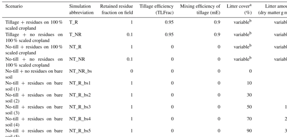
Table 1.LPJmL simulation settings and tillage parameters used in the stylized simulations for model evaluation.
Scenario Simulation Retained residue Tillage efficiency Mixing efficiency of Litter covera Litter amount abbreviation fraction on field (TLFrac) tillage (mE) (%) (dry matter g m2) Tillage+residues on 100 %
scaled cropland
T_R 1 0.95 0.9 variableb variableb Tillage + no residues on
100 % scaled cropland
T_NR 0.1 0.95 0.9 variableb variableb No-till+residues on 100 %
scaled cropland
NT_R 1 0 0 variableb variableb
No-till + no residues on 100 % scaled cropland
NT_NR 0.1 0 0 variableb variableb No-till+no residues on bare
soil
NT_NR_bs 0 0 0 0 0
No-till + residues on bare soil (1)
NT_R_bs1 1 0 0 10 17
No-till + residues on bare soil (2)
NT_R_bs2 1 0 0 30 60
No-till + residues on bare soil (3)
NT_R_bs3 1 0 0 50 117
No-till + residues on bare soil (4)
NT_R_bs4 1 0 0 70 202
No-till + residues on bare soil (5)
NT_R_bs5 1 0 0 90 383
aLitter cover is calculated following Gregory (1982).bLitter amounts and litter cover are modelled internally.
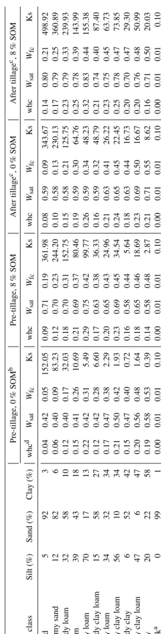
Clay soils are an exception, since higher SOM content de-creases whc,Wsat,l, andWfc,l, and increases Ksl. The effect
of increasing SOM content on whc,Wsat,l, andWfc,lis
great-est in the soil classes sand and loamy sand. The increasing effects of tillage on the hydraulic properties are generally weaker compared to an increase in SOM by 8 % (maximum SOM content for computing soil hydraulic properties in the model). While tillage (mE of 0.9, 0 % SOM) in sandy soils increase whc by 83 %, 8 % of SOM can increase whc in an untilled soil by 105 % and in a tilled soil by 84 %. As com-parison, in silty loam soils with 0 % SOM, tillage (mE of 0.9) increases whc by 16 %, while 8 % SOM can increase whc by 31 % and by 26 % for untilled and tilled soil, respectively.
The PTF by Saxton and Rawls (2006) uses an empirical relationship between SOM, soil texture, and hydraulic prop-erties derived from the USDA soil database, implying that the PTF is likely to be more accurate within the US than out-side. A PTF developed for global-scale application is, to our knowledge, not yet developed. Nevertheless PTFs are used in a variety of global applications, despite the limitations to validate at this scale (Van Looy et al., 2017).
5.2 Productivity
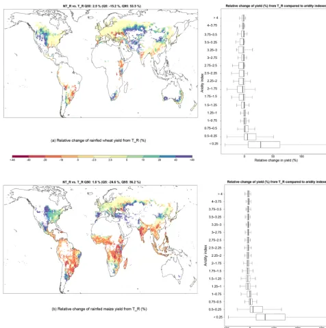
In our simulations, adopting NT_R slightly increases produc-tivity for all rain-fed crops simulated (wheat, maize, pulses, rapeseed) on average, but ranges from increases to decreases across all cropland globally. This increase can be observed for the first 3 years (Fig. S2 in the Supplement), and for the first 10 years (Fig. 2a and b). All the results shown here and in the subsequent sections are calculated as RD following
Figure 2.Relative yield changes for rain-fed wheat(a)and rain-fed maize(b)compared to aridity indexes after 10 years NT_R vs. T_R. Low aridity index values indicate arid conditions as the index is defined as mean annual precipitation divided by potential evapotranspiration,
following Pittelkow et al. (2015a). Substantial increases in crop yields only occur in arid regions, with aridity indices<0.75.
and decreases in evaporation. Areas where crop productiv-ity is limited by soil water could therefore potentially ben-efit from NT_R (Pittelkow et al., 2015a). The influence of climatic condition of no-till effects on productivity was al-ready found by several other studies (e.g. Ogle et al., 2012; Pittelkow et al., 2015a; van Kessel et al., 2013). Ogle et al. (2012) found declines in productivity but these declines were larger in the cooler and wetter climates. Pittelkow et al. (2015a) found only small declines in productivity in dry
T able 2. Percentage v alues for each soil te xtural class of silt, sand and clay content used in LPJmL and correspondent h ydraulic parameters before and after tillage with 0 % and 8 % SOM using the Saxton and Ra wls (2006) pedotransfer function. Pre-tillage, 0 % SOM b Pre-tillage, 8 % SOM After tillage c, 0 % SOM After tillage c, 8 % SOM Soil class Silt (%) Sand (%) Clay (%) whc d W sat W fc Ks whc Wsat Wfc Ks whc W sat W fc Ks whc Wsat W fc Ks Sand 5 92 3 0.04 0.42 0.05 152.05 0.09 0.71 0.19 361.98 0.08 0.59 0.09 343.67 0.14 0.80 0.21 498.92 Loamy sand 12 82 6 0.06 0.40 0.09 83.23 0.12 0.70 0.23 244.20 0.10 0.58 0.13 230.13 0.17 0.79 0.25 360.89 Sandy loam 32 58 10 0.12 0.40 0.17 32.03 0.18 0.70 0.31 152.75 0.15 0.58 0.21 125.75 0.23 0.79 0.33 239.93 Loam 39 43 18 0.15 0.41 0.26 10.69 0.21 0.69 0.37 80.46 0.19 0.59 0.30 64.76 0.25 0.78 0.39 143.99 Silty loam 70 17 13 0.22 0.42 0.31 5.49 0.29 0.75 0.42 99.77 0.26 0.59 0.34 48.23 0.32 0.83 0.44 155.38 Sandy clay loam 15 58 27 0.12 0.42 0.28 6.60 0.17 0.63 0.38 36.33 0.16 0.59 0.32 48.79 0.21 0.74 0.40 87.40 Clay loam 34 32 34 0.17 0.47 0.38 2.29 0.20 0.65 0.43 24.96 0.21 0.63 0.41 26.22 0.23 0.75 0.45 63.73 Silty clay loam 56 10 34 0.21 0.50 0.42 1.93 0.23 0.69 0.45 34.54 0.24 0.65 0.45 22.45 0.25 0.78 0.47 73.85 Sandy clay 6 52 42 0.15 0.47 0.40 0.72 0.16 0.58 0.44 5.64 0.18 0.63 0.44 16.73 0.20 0.70 0.47 29.30 Silty clay loam 47 6 47 0.20 0.56 0.48 1.64 0.18 0.65 0.46 18.69 0.23 0.69 0.50 16.67 0.20 0.76 0.48 50.99 Clay 20 22 58 0.19 0.58 0.53 0.39 0.14 0.58 0.48 2.87 0.21 0.71 0.55 8.62 0.16 0.71 0.50 20.03 Rock a 0 99 1 0.00 0.01 0.01 0.10 0.00 0.01 0.01 0.10 0.00 0.01 0.01 0.10 0.00 0.01 0.01 0.10 aSoil class rock is not af fected by SOM changes and tillage practices. bF or SOM we only consider the C part in SOM in grammes of carbon per square metre (gC m − 2) . cT illage with a mE of 0.9 for con v entional tillage. dwhc is calculated as whc = Wfc − Wpwp in all cases.
crop residues are treated in no-till and tillage (i.e. removed or retained).
Negative effects of NT_R on productivity can be ob-served in mainly tropical areas. As soil moisture increases in tropical areas under NT_R as well (Fig. 5c), the decline is resulting from a decrease in N availability in the soil (Fig. 5d). Soil moisture drives many N-related processes that can cause a decline in N. For instance, the increase in soil moisture can lead to an increase in denitrification, which de-creases the amount of NO−3 (which will be discussed fur-ther in Sect. 5.5). On the ofur-ther hand, mineralization can also be reduced if soil moisture is too high. However, the soil-moisture–N availability and yield feedback is complex as many processes are involved.
5.3 Soil C stocks and fluxes
meta-analyses conducted by Pittelkow et al. (2015b), who report a positive effect on yields (and thus general produc-tivity and thus C input) of no-till compared to conventional tillage in dry climates. Their results show that, in general, no-till performs best relative to conventional tillage under water-limited conditions, due to enhanced water-use efficien-cies when residues are retained.
Abdalla et al. (2016) reviewed the effect of tillage, no-till, and residue management and found that if residues are re-turned, no-till compared to conventional tillage increases soil and litter C content by 5.0 % (95th CI:−1.0 %,+9.2 %) and decreases CO2 emissions from soils by−23.0 % (95th CI: −35.0 %,−13.8 %) (Table 3). These findings of Abdalla et al. (2016) are in line with our findings for CO2 emissions if we consider the first 3 years of duration for CO2 emis-sions and 10 years duration for topsoil and litter C. Abdalla et al. (2016) do not explicitly specify a time of duration for these results. If we only analyse the tillage effect without taking residues into account (T_NR vs. NT_NR), we find in our simulation that topsoil and litter C decreases by−18.0 % (5th, 95th percentile:−42.5 %,−0.5 %) after 20 years, while CO2 emissions increase by+21.3 % (5th, 95th percentile: −1.1 %,+125.2 %) mostly in humid regions (Table 3). Ab-dalla et al. (2016) also reported soil and litter C changes from a T_NR vs. NT_NR comparison and reported a decrease in soil and litter C under T_NR of−12.0 % (95th CI:−15.3 %, −5.1 %) and a CO2increase of+18.0 % (95th CI:+9.4 %, +27.3 %), which is well in line with our model results.
Ogle et al. (2005) conducted a meta-analysis and reported SOC changes from NT_R compared to T_R system with medium C input, grouped for different climatic zones. They found a+23 %,+17 %,+16 %, and+10 % mean increase in SOC after converting from a conventional tillage to a no-till system for more than 20 years for tropical moist, tropical dry, temperate moist, and temperate dry climates, respectively. We only find a+4.8 %,+8.3 %,+3.5 %, and+5.8 % mean increase in topsoil and litter C for these regions, respectively. However, Ogle et al. (2005) analysed the data by comparing a no-till system with high C inputs from rotation and residues to a conventional tillage system with medium C input from rotation and residues. We compare two similarly productive systems with each other, where residues are either left on the field or incorporated through tillage (NT_R vs. T_R), which may explain why we see smaller relative effects in the sim-ulations. Comparing a high input system with a medium or a low input system will essentially lead to an amplification of soil and litter C changes over time; nevertheless, we are still able to generally reproduce a SOC increase over longer periods.
Unfortunately there are high discrepancies in the litera-ture with regard to no-till effects on soil and litter C, since the high increases found by Ogle et al. (2005) are not sup-ported by the findings of Abdalla et al. (2016). Ranaivoson et al. (2017) found that crop residues left on the field increases
soil and litter C content, which is in agreement with our sim-ulation results.
5.4 Water fluxes
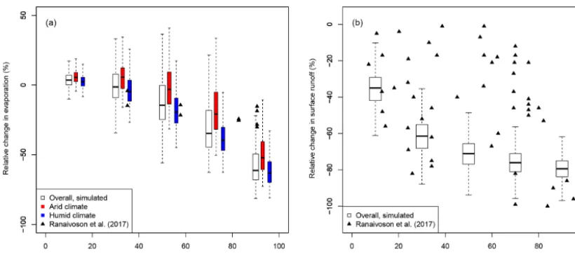
We evaluate the effects of tillage and residue management on water fluxes by analysing soil evaporation and surface runoff. Our results show that evaporation and surface runoff under NT_R compared to T_R are generally reduced by −44.3 % (5th, 95th percentiles: −64.5, −17.4 %) and by −57.8 % (5th, 95th percentiles:−74.6 %,−26.1 %), respec-tively (Fig. S4a and b in the Supplement). We also analysed soil evaporation and surface runoff for different amounts of surface litter loads and cover on bare soil without vegetation in order to compare our results to literature estimates from field experiments. We find that both the reduction in evapo-ration and surface runoff are dependent on the residue load, which translates into different rates of surface litter cover.
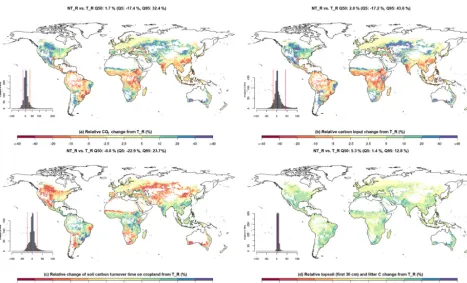
Ranaivo-Figure 3.Relative C dynamics for NT_R vs. T_R comparison after 10 years of simulation experiment (average of year 9–11) for relative
CO2change(a), relative C input change(b), relative change of soil C turnover time(c), and relative topsoil and litter C change(d).
son et al. (2017) for up to 70 % soil cover, especially when analysing humid climates. For higher soil cover≥70 %, the model seems to be more in line with literature values for arid regions. Overall for high soil cover of 90 %, the model seems to overestimate the reduction of evaporation. It should be noted that the estimates from Ranaivoson et al. (2017) are only taken from two field studies, which are only rep-resentative for the local climatic and soil conditions, since global data on the effect of surface litter on evaporation are not available. The general effect of surface litter on the re-duction in soil evaporation is thus captured by the model, but the model seems to overestimate the response at high litter loads. It is not entirely clear from the literature if these ex-periments have been carried out on bare soil without vegeta-tion. If crops are also grown in the experiments, water can be used for transpiration which is otherwise available for evap-oration, which could explain why the model overestimates the effect of surface litter on evaporation on bare soil without any vegetation.
Ranaivoson et al. (2017) also investigated the runoff re-duction under soil cover, but the results do not show a clear picture. In theory, surface litter reduces surface runoff and the literature generally supports this assumption (Kurothe et al., 2014; Wilson et al., 2008), but the magnitude of the effect varies. Figure 4b compares our modelled results under dif-ferent soil cover to the literature values from Ranaivoson et al. (2017). This shows that modelled results across all global
cropland are on the upper end of the effect of surface runoff reduction from soil cover, but they are still well within the range reported by Ranaivoson et al. (2017). The amount of water which is infiltrated (and thus not going into surface runoff) is affected by the parameterpin Eq. (11), which is dependent on the amount of surface litter cover (fsurf). The parameterization ofp is chosen to be at the upper end of the approach by Jägermeyr et al. (2016) at full surface lit-ter cover, as this should substantially reduce surface runoff (Tapia-Vargas et al., 2001) and thus increase infiltration rates (Strudley et al., 2008). The parametrization ofpcan be ad-justed if better site-specific information on slope, soils crust-ing, and rainfall intensity is available.
5.5 N2O fluxes
Switching from tillage to no-till management with leaving residues on the fields (NT_R vs. T_R) increases N2O emis-sions by a median of+20.8 % (5th, 95th percentile:−3.6 %, +325.5 %) (Fig. S6a in the Supplement). The strongest in-crease is found in the cool temperate zone where the av-erage increase is +23.5 % (5th, 95th percentile: −0.1 %, +664.4 %) (Fig. S6e in the Supplement). The lowest increase is found in the tropical zone+15.8 % (5th, 95th percentile: −7.3 %,+72.1 %) (Fig. S6c in the Supplement).
Do-Figure 4.Relative change in evaporation(a)and surface runoff(b)relative to soil cover from surface residues for different soil cover values of 10 %, 30 %, 50 %, 70 %, and 90 % (simulation NT_R_bs1 to NT_R_bs5 vs. NT_NR_bs, respectively). For better visibility, the red and blue boxplots are plotted next to the overall boxplots, but correspond to the soil cover value of the overall simulation (empty boxes).
ran, 1984; Mei et al., 2018; van Kessel et al., 2013; Zhao et al., 2016) (Table 3). Mei et al. (2018) reports an over-all increase of+17.3 % (95th CI:+4.6 %,+31.1 %), which is in agreement with our median estimate. However, the re-gional patterns over the different climatic regimes are in less agreement. LPJmL simulations strongly underestimate the increase in N2O emissions in the tropical zone, whereas sim-ulations overestimate the response in cool temperate and hu-mid zones and to some extent in the warm temperate zone (Table 3).
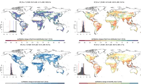
In general, N2O emissions are formed in two separate pro-cesses: nitrification and denitrification. The increase in N2O emissions after adapting to NT_R is mainly resulting from denitrification in our simulations (+55.9 %, Fig. 5a). This increase is visible in most of the regions. The N2O emis-sions resulting from nitrification decrease mostly (median of −6.0 %, Fig. 5b) but tends to increase in dry areas. The in-crease in denitrification and dein-crease in nitrification, results in a decrease in NO−3 (median of−26.4 %), which appears to be stronger in the tropical areas as well (Fig. 5d). The trans-formation of mineral N to N2O is not only affected by the nitrification and denitrification rates, but also by substrate availability (NH+4 and NO−3). These in turn are affected by nitrification and denitrification rates, but also by other pro-cesses, such as plant uptake and leaching. In the Sahel zone, for example, denitrification decreases and nitrification in-creases, but NO−3 stocks decline, because leaching increases more strongly (Fig. S7 in the Supplement).
In LPJmL, denitrification and nitrification rates are mainly driven by soil moisture and to a lesser extent by soil tem-perature, soil C (denitrification), and soil pH (nitrification). A strong increase in annually averaged soil moisture can be observed after adapting NT_R (median of+18.9 %, Fig. 5c). Denitrification, as an anoxic process, increases non-linearly
beyond a soil moisture threshold (von Bloh et al. 2018), whereas there is an optimum soil moisture for nitrification, which is reduced at low and high soil moisture contents. In wet regions, as in the tropical and humid areas, nitrification is thus reduced by no-till practices, whereas it increases in dryer regions. The increase in soil moisture under NT_R is caused by higher water infiltration rates and reduced soil evapora-tion (see Sect. 5.4). Also, no-till practices tend to increase bulk density and thus higher relative soil moisture contents (Fig. 1) also affecting nitrification and denitrification rates and therefore N2O emissions (van Kessel et al., 2013; Linn and Doran, 1984).
Empirical evidence shows that the introduction of no-till practices on N2O emissions can cause both increases and de-creases in N2O emissions (van Kessel et al., 2013). This vari-ation in response is not surprising, as tillage affects several biophysical factors that influence N2O emissions (Fig. 1) in possibly contrasting manners (van Kessel et al., 2013; Snyder et al., 2009). For instance, no-till can lower soil temperature exchange between soil and atmosphere through the presence of litter residues, which can reduce N2O emissions (Enrique et al., 1999). Reduced N2O emissions under no-till compared to tillage MS can also be observed in the model results, for instance in northern Europe and areas in Brazil (Fig. S6a in the Supplement).
As several biophysical factors are affected, N2O emissions are characterized by significant spatial and temporal variabil-ity. As a result, the estimation of N2O emissions are accom-panied with high uncertainties (Butterbach-Bahl et al., 2013), which hamper the evaluation of the model results (Chatskikh et al., 2008; Mangalassery et al., 2015).
Figure 5.Relative changes for the average of the first 3 years of NT_R vs. T_R for denitrification(a), nitrification(b), soil water content(c),
and NO−3 (d).
and verification, including model simulations for specific sites at which experiments have been conducted. The sen-sitivity of N2O emissions highlights the importance of cor-rectly simulating soil moisture. However, simulating soil moisture is subject to strong feedback with vegetation per-formance and comes with uncertainties, as addressed by, for example, Seneviratne et al. (2010). The effects of different management settings (as conducted here) on N2O emissions and soil moisture therefore requires further analyses, ideally in different climate regimes, soil types, and in combination with other management settings (e.g. N fertilizers). We ex-pect that further studies using this tillage implementation in LPJmL will increase the understanding of management ef-fects on soil nitrogen dynamics. The great diversity in ob-served responses in N2O emissions to management options (Mei et al., 2018) renders modelling these effects as chal-lenging, but we trust that the ability of LPJmL5.0-tillage to represent the different components can also help to better un-derstand their interaction under different environmental con-ditions.
5.6 General discussion
The implementation of tillage into the global ecosystem model LPJmL opens up opportunities to assess the effects of different tillage practices on agricultural productivity and its environmental impacts, such as nutrient cycles, water
con-sumption, GHG emissions, and C sequestration and is a gen-eral model improvement to the previous version of LPJmL (von Bloh et al., 2018). The implementation involved (1) the introduction of a surface litter pool that is incorporated into the soil column at tillage events and the subsequent effects on soil evaporation and infiltration, (2) dynamically accounting for SOM content in computing soil hydraulic properties, and (3) simulating tillage effects on bulk density and the subse-quent effects of changed soil water properties and all water-dependent processes (Fig. 1).
We find that the model results for NT_R compared to T_R are generally in agreement with literature with regard to mag-nitude and direction of the effects on C stocks and fluxes. De-spite some disagreement between reported ranges in effects and model simulations, we find that the diversity in mod-elled responses across environmental gradients is an asset of the model. The underlying model mechanisms, such as the initial decrease in CO2emissions after introduction of no-till practices, can be maintained for longer time periods in moist regions, but are inverted in dry regions due to the feedback of higher water availability on plant productivity and reduced turnover times, and generally increasing soil carbon stocks (Fig. 3) are plausible and in line with general process under-standing. Certainly, the interaction of the different processes may not be captured correctly and further research on this is needed. We trust that this model implementation represent-ing this complexity allows for further research in this direc-tion. For water fluxes, the model seems to overestimate the effect of surface residue cover on evaporation for high sur-face cover, but the evaluation is also constrained by the small number of suitable field studies. Effects can also change over time so that a comparison needs to consider the timing, his-tory, and duration of management changes and specific lo-cal climatic and soil conditions. The overall effect of NT_R compared to T_R on N2O emissions is in agreement with lit-erature as well. However, the regional patterns over the dif-ferent climatic regimes are in less agreement. N2O emissions are highly variable in space and time and are very sensitive to soil water dynamics (Butterbach-Bahl et al., 2013). The simulation of soil water dynamics differs per soil type as the calculation of the hydraulic parameters is texture specific. Moreover, these parameters are now changed after a tillage event. The effects of tillage on N2O emissions, as well as other processes that are driven by soil water (e.g. CO2, water dynamics), can therefore be different per soil type. The soil-specific effects of tillage on N2O and CO2emissions was al-ready studied by Abdalla et al. (2016) and Mei et al. (2018). Abdalla et al. (2016) found that differences in CO2emissions between tilled and untilled soils are largest in sandy soils (+29 %), whereas the differences in clayey soils are much smaller (+12 %). Mei et al. (2018) found that clay content <20 % significantly increases N2O emissions (+42.9 %) af-ter adapting to conservation tillage, whereas this effect for clay content>20 % is smaller (+2.9 %). These studies show that soil-type-specific tillage effects on several processes can be of importance and should be investigated in more detail in future studies. The interaction of all relevant processes is complex, as seen in Fig. 1, which can also lead to high un-certainties in the model. Again, we think that this model im-plementation captures substantial aspects of this complexity and thus lays the foundation for further research.
It is important to note that not all processes related to tillage and no-till are taken into account in the current model implementation. For instance, NT_R can improve soil struc-ture (e.g. aggregates) due to increased faunal activity
(Mar-tins et al., 2009), which can result in a decrease in BD. Al-though tillage can have several advantages for the farmer, e.g. residue incorporation and topsoil loosening, it can also have several disadvantages. For instance, tillage can cause com-paction of the subsoil (Bertolino et al., 2010), which results in an increase in BD (Podder et al., 2012) and creates a bar-rier for percolating water, leading to ponding and an oversat-urated topsoil. Strudley et al. (2008), however, observed di-verging effects of tillage and no-till on hydraulic properties, such as BD, Ks, and whc for different locations. They ar-gue that affected processes of agricultural management have complex coupled effects on soil hydraulic properties; also, that variations in space and time often lead to higher differ-ences than the measured differdiffer-ences between the manage-ment treatmanage-ments. They further argue that characteristics of soil type and climate are unique for each location, which cannot simply be transferred from one field location to an-other. A process-based representation of tillage effects as in this extension of LPJmL allows for further studying of man-agement effects across diverse environmental conditions, but also to refine model parameters and implementations where experimental evidence suggests disagreement.
One of the primary reasons for tillage, weed control, is also not accounted for in LPJmL5.0-tillage or in other ecosystem models. As such, different tillage and residue management strategies can only be assessed with respect to their biogeo-chemical effects, but only partly with respect to their effects on productivity and not with respect to some environmen-tal effects (e.g. pesticide use). Our model simulations show that crop yields increase under no-till practices in dry areas but decrease in wetter regions (Fig. 2). However, the median response is positive, which may be in part because the wa-ter saving effects from increased soil cover with residues are overestimated or because detrimental effects, such as compe-tition with weeds, are not accounted for.
pro-cesses, such as erosion, data availability, and model structure, need to be considered in further model development (Lutz et al., 2019). As such, some processes, such as a detailed repre-sentation of soil crusting processes, may remain out of reach for global-scale modelling.
6 Conclusions
We described the implementation of tillage-related processes into the global ecosystem model LPJmL5.0-tillage. The ex-tended model was tested under different management sce-narios and evaluated by comparing to reported impact ranges from meta-analyses on C, water, and N dynamics, as well as on crop yields.
We find that mostly arid regions benefit from a no-till man-agement with leaving residues on the field, due to the water saving effects of surface litter. We are able to broadly repro-duce reported tillage effects on global stocks and fluxes, as well as regional patterns of these changes with LPJmL5.0-tillage, but deviations in N fluxes need to be further exam-ined. Not all effects of tillage – including one of its pri-mary reasons, weed control – could be accounted for in this implementation. Uncertainties mainly arise because of the multiple feedback mechanisms affecting the overall response to tillage, especially as most processes are affected by soil moisture. The processes and feedbacks presented in this im-plementation are complex and evaluation of effects is often limited to the availability of reference data. Nonetheless, the implementation of more detailed tillage-related mechanics into the LPJmL global ecosystem model improves our ability to represent different agricultural systems and to understand management options for climate change adaptation, agricul-tural mitigation of GHG emissions, and sustainable intensifi-cation. We trust that this model implementation and the pub-lication of the underlying source code will promote research on the role of tillage for agricultural production, its environ-mental impact, and global biogeochemical cycles.
Code and data availability. The source code is publicly avail-able under the GNU AGPL version 3 license. An exact ver-sion of the source code described here is archived under https://doi.org/10.5281/zenodo.2652136 (Herzfeld et al., 2019).
Supplement. The supplement related to this article is available online at: https://doi.org/10.5194/gmd-12-2419-2019-supplement.
Author contributions. FL and TH both share the lead authorship for this paper. They had equal input in designing and conducting the model implementation, model runs, analysis, and writing of the pa-per. SR contributed to simulation analysis and paper preparation and evaluation. JH contributed to the code implementation, evaluation, and analysis, and edited the paper. SS contributed to the code
im-plementation and evaluation and edited the paper. WvB contributed to the code implementation and evaluation and edited the paper. JJS contributed to the study design and edited the paper. CM contributed to the study design and supervised the implementation, simulations, and analyses, and also edited the paper.
Competing interests. The authors declare that they have no conflict of interest.
Acknowledgements. Femke Lutz, Tobias Herzfeld, and Susanne Rolinski gratefully acknowledge the German Ministry for Educa-tion and Research (BMBF) for funding this work, which is part of the MACMIT project (01LN1317A). Jens Heinke acknowledges BMBF funding through the SUSTAg project (031B0170A). We thank Quazi Rasool and one anonymous referee for their helpful comments on earlier versions of the paper.
Financial support. This research has been supported by the BMBF (grant no. 01LN1317A) and through SUSTAg (grant no. 031B0170A).
The article processing charges for this open-access publica-tion were covered by the Potsdam Institute for Climate Impact Research (PIK).
Review statement. This paper was edited by Havala Pye and re-viewed by Quazi Rasool and one anonymous referee.
References
Abdalla, K., Chivenge, P., Ciais, P., and Chaplot, V.: No-tillage
lessens soil CO2emissions the most under arid and sandy soil
conditions: results from a meta-analysis, Biogeosciences, 13, 3619–3633, https://doi.org/10.5194/bg-13-3619-2016, 2016. Armand, R., Bockstaller, C., Auzet, A.-V., and Van Dijk, P.: Runoff
generation related to intra-field soil surface characteristics vari-ability: Application to conservation tillage context, Soil Till. Res., 102, 27–37, https://doi.org/10.1016/j.still.2008.07.009, 2009.
Aslam, T., Choudhary, M. A., and Saggar, S.: Influence of
land-use management on CO2 emissions from a silt loam
soil in New Zealand, Agr. Ecosyst. Environ., 77, 257–262, https://doi.org/10.1016/S0167-8809(99)00102-4, 2000. Balland, V., Pollacco, J. A. P., and Arp, P. A.:
Mod-eling soil hydraulic properties for a wide range
of soil conditions, Ecol. Model., 219, 300–316,
https://doi.org/10.1016/j.ecolmodel.2008.07.009, 2008. Batjes, N.: ISRIC-WISE global data set of derived soil properties
on a 0.5 by 0.5 degree grid (version 3.0), ISRIC – World Soil Information, Wageningen, 2005.
Precipita-tion Climatology Centre with sample applicaPrecipita-tions including cen-tennial (trend) analysis from 1901–present, Earth Syst. Sci. Data, 5, 71–99, https://doi.org/10.5194/essd-5-71-2013, 2013. Bertolino, A. V. F. A., Fernandes, N. F., Miranda, J. P. L., Souza,
A. P., Lopes, M. R. S., and Palmieri, F.: Effects of plough pan development on surface hydrology and on soil physical proper-ties in Southeastern Brazilian plateau, J. Hydrol., 393, 94–104, https://doi.org/10.1016/j.jhydrol.2010.07.038, 2010.
Best, M. J., Pryor, M., Clark, D. B., Rooney, G. G., Essery, R. L. H., Ménard, C. B., Edwards, J. M., Hendry, M. A., Porson, A., Gedney, N., Mercado, L. M., Sitch, S., Blyth, E., Boucher, O., Cox, P. M., Grimmond, C. S. B., and Harding, R. J.: The Joint UK Land Environment Simulator (JULES), model description – Part 1: Energy and water fluxes, Geosci. Model Dev., 4, 677–699, https://doi.org/10.5194/gmd-4-677-2011, 2011.
Bondeau, A., Smith, P. C., Zaehle, S., Schaphoff, S., Lucht, W., Cramer, W., Gerten, D., Lotze-Campen, H., MüLler, C., Re-ichstein, M., and Smith, B.: Modelling the role of agricul-ture for the 20th century global terrestrial carbon balance, Glob. Change Biol., 13, 679–706, https://doi.org/10.1111/j.1365-2486.2006.01305.x, 2007.
Brady, N. C. and Weil, R. R.: The nature and properties of soils, Pearson Prentice Hall Upper Saddle River, 2008.
Butterbach-Bahl, K., Baggs, E. M., Dannenmann, M., Kiese, R., and Zechmeister-Boltenstern, S.: Nitrous oxide emissions from soils: how well do we understand the processes and their controls?, Philos. T. Roy. Soc. B, 368, 20130122, https://doi.org/10.1098/rstb.2013.0122, 2013.
Chatskikh, D., Olesen, J. E., Hansen, E. M., Elsgaard, L., and Petersen, B. M.: Effects of reduced tillage on net greenhouse gas fluxes from loamy sand soil under winter crops in Denmark, Agr. Ecosyst. Environ., 128, 117–126, https://doi.org/10.1016/j.agee.2008.05.010, 2008.
Chen, H., Hou, R., Gong, Y., Li, H., Fan, M., and
Kuzyakov, Y.: Effects of 11 years of conservation tillage on soil organic matter fractions in wheat monoculture in Loess Plateau of China, Soil Till. Res., 106, 85–94, https://doi.org/10.1016/j.still.2009.09.009, 2009.
Ciais, P., Gervois, S., Vuichard, N., Piao, S. L., and Viovy, N.: Effects of land use change and management on the European cropland carbon balance, Glob. Change Biol., 17, 320–338, https://doi.org/10.1111/j.1365-2486.2010.02341.x, 2011. Clark, D. B., Mercado, L. M., Sitch, S., Jones, C. D., Gedney, N.,
Best, M. J., Pryor, M., Rooney, G. G., Essery, R. L. H., Blyth, E., Boucher, O., Harding, R. J., Huntingford, C., and Cox, P. M.: The Joint UK Land Environment Simulator (JULES), model description – Part 2: Carbon fluxes and vegetation dynamics, Geosci. Model Dev., 4, 701–722, https://doi.org/10.5194/gmd-4-701-2011, 2011.
Cosby, B. J., Hornberger, G. M., Clapp, R. B., and Ginn, T. R.: A Statistical Exploration of the Relationships of Soil Moisture Characteristics to the Physical Properties of Soils, Water Resour. Res., 20, 682–690, https://doi.org/10.1029/WR020i006p00682, 1984.
Daigh, A. L. M. and DeJong-Hughes, J.: Fluffy soil syndrome: When tilled soil does not settle, J. Soil Water Conserv., 72, 10A– 14A, https://doi.org/10.2489/jswc.72.1.10A, 2017.
Dee, D. P., Uppala, S. M., Simmons, A. J., Berrisford, P., Poli, P., Kobayashi, S., Andrae, U., Balmaseda, M. A., Balsamo, G.,
Bauer, P., Bechtold, P., Beljaars, A. C. M., Berg, L. van de, Bid-lot, J., Bormann, N., Delsol, C., Dragani, R., Fuentes, M., Geer, A. J., Haimberger, L., Healy, S. B., Hersbach, H., Hólm, E. V., Isaksen, L., Kållberg, P., Köhler, M., Matricardi, M., McNally, A. P., Monge-Sanz, B. M., Morcrette, J.-J., Park, B.-K., Peubey, C., Rosnay, P. de, Tavolato, C., Thépaut, J.-N., and Vitart, F.: The ERA-Interim reanalysis: configuration and performance of the data assimilation system, Q. J. Roy. Meteor. Soc., 137, 553–597, https://doi.org/10.1002/qj.828, 2011.
Elliott, J., Müller, C., Deryng, D., Chryssanthacopoulos, J., Boote, K. J., Büchner, M., Foster, I., Glotter, M., Heinke, J., Iizumi, T., Izaurralde, R. C., Mueller, N. D., Ray, D. K., Rosenzweig, C., Ruane, A. C., and Sheffield, J.: The Global Gridded Crop Model Intercomparison: data and modeling protocols for Phase 1 (v1.0), Geosci. Model Dev., 8, 261–277, https://doi.org/10.5194/gmd-8-261-2015, 2015.
Enrique, G. S., Braud, I., Jean-Louis, T., Michel, V., Pierre, B., and Jean-Christophe, C.: Modelling heat and water ex-changes of fallow land covered with plant-residue mulch, Agr. Forest Meteorol., 97, 151–169, https://doi.org/10.1016/S0168-1923(99)00081-7, 1999.
Fader, M., Rost, S., Müller, C., Bondeau, A., and Gerten, D.: Virtual water content of temperate cereals and maize: Present and potential future patterns, J. Hydrol., 384, 218–231, https://doi.org/10.1016/j.jhydrol.2009.12.011, 2010.
Friend, A. D., Lucht, W., Rademacher, T. T., Keribin, R., Betts, R., Cadule, P., Ciais, P., Clark, D. B., Dankers, R., Fal-loon, P. D., Ito, A., Kahana, R., Kleidon, A., Lomas, M. R., Nishina, K., Ostberg, S., Pavlick, R., Peylin, P., Schaphoff, S., Vuichard, N., Warszawski, L., Wiltshire, A., and Wood-ward, F. I.: Carbon residence time dominates uncertainty in terrestrial vegetation responses to future climate and
atmo-spheric CO2, P. Natl. Acad. Sci. USA, 111, 3280–3285,
https://doi.org/10.1073/pnas.1222477110, 2014.
Glab, T. and Kulig, B.: Effect of mulch and tillage system on soil porosity under wheat (Triticum aestivum), Soil Till. Res., 99, 169–178, https://doi.org/10.1016/j.still.2008.02.004, 2008. Govers, G., Vandaele, K., Desmet, P., Poesen, J., and Bunte, K.: The
role of tillage in soil redistribution on hillslopes, Eur. J. Soil Sci., 45, 469–478, 1994.
Green, T. R., Ahuja, L. R., and Benjamin, J. G.: Advances and challenges in predicting agricultural management ef-fects on soil hydraulic properties, Geoderma, 116, 3–27, https://doi.org/10.1016/S0016-7061(03)00091-0, 2003. Gregory, J. M.: Soil cover prediction with various amounts
and types of crop residue, T. ASAE, 25, 1333–1337, https://doi.org/10.13031/2013.33723, 1982.
Guérif, J., Richard, G., Dürr, C., Machet, J. M., Recous, S., and Roger-Estrade, J.: A review of tillage effects on crop residue management, seedbed conditions and seedling establishment, Soil Till. Res., 61, 13–32, 2001.
Harris, I., Jones, P. D., Osborn, T. J., and Lister, D. H.: Up-dated high-resolution grids of monthly climatic observations – the CRU TS3.10 Dataset, Int. J. Climatol., 34, 623–642, https://doi.org/10.1002/joc.3711, 2014.