www.geosci-instrum-method-data-syst.net/2/275/2013/ doi:10.5194/gi-2-275-2013
© Author(s) 2013. CC Attribution 3.0 License.
Instrumentation
Methods and
Data Systems
Automated field detection of rock fracturing, microclimate, and
diurnal rock temperature and strain fields
K. Warren1, M.-C. Eppes2, S. Swami3, J. Garbini1, and J. Putkonen4
1UNC Charlotte, Civil and Environmental Engineering Department, 9201 University City Boulevard, Charlotte, NC 28223-0001, USA
2UNC Charlotte, Department of Geography and Earth Sciences, 9201 University City Boulevard, Charlotte, NC 28223-0001, USA
3UNC Charlotte, Department of Electrical and Computing Engineering, 9201 University City Boulevard, Charlotte, NC 28223-0001, USA
4Harold Hamm School of Geology and Geological Engineering, 101 Leonard Hall, 81 Cornell St. – Stop 8358, University of North Dakota, Grand Forks, ND 58202-8358, USA
Correspondence to: M.-C. Eppes ([email protected])
Received: 4 April 2013 – Published in Geosci. Instrum. Method. Data Syst. Discuss.: 2 July 2013 Revised: 10 October 2013 – Accepted: 18 October 2013 – Published: 27 November 2013
Abstract. The rates and processes that lead to non-tectonic rock fracture on Earth’s surface are widely debated but poorly understood. Few, if any, studies have made the direct observations of rock fracturing under natural conditions that are necessary to directly address this problem. An instrumen-tation design that enables concurrent high spatial and tempo-ral monitoring resolution of (1) diurnal environmental con-ditions of a natural boulder and its surroundings in addition to (2) the fracturing of that boulder under natural full-sun exposure is described herein. The surface of a fluvially trans-ported granite boulder was instrumented with (1) six acous-tic emission (AE) sensors that record micro-crack associated, elastic wave-generated activity within the three-dimensional space of the boulder, (2) eight rectangular rosette foil strain gages to measure surface strain, (3) eight thermocouples to measure surface temperature, and (4) one surface moisture sensor. Additionally, a soil moisture probe and a full weather station that measures ambient temperature, relative humid-ity, wind speed, wind direction, barometric pressure, insola-tion, and precipitation were installed adjacent to the test boul-der. AE activity was continuously monitored by one logger while all other variables were acquired by a separate logger every 60 s. The protocols associated with the instrumenta-tion, data acquisiinstrumenta-tion, and analysis are discussed in detail. During the first four months, the deployed boulder experi-enced almost 12 000 AE events, the majority of which occur
in the afternoon when temperatures are decreasing. This pa-per presents preliminary data that illustrates data validity and typical patterns and behaviors observed. This system offers the potential to (1) obtain an unprecedented record of the nat-ural conditions under which rocks fracture and (2) decipher the mechanical processes that lead to rock fracture at a vari-ety of temporal scales under a range of natural conditions.
1 Introduction
required to demonstrate an unequivocal correlation between environmental factors and rock fracturing. Such correlations are necessary to decode processes responsible for rock frac-ture, and to calculate them, one would need a simultaneous record of both fracturing and the environmental conditions of the rock at the time that the fracture occurred. For example, if freeze–thaw is the primary driver of rock fracture, there should be a temporal correlation between the time that frac-turing occurs and the time that the temperature of the rock drops below freezing. If directional insolation (McFadden et al., 2005) is driving rock fracture, there should be a spa-tial and temporal correlation between patterns of tempera-ture driven strain and fracturing on the rock. An experimental configuration capable of monitoring rock fracturing in such a way would be useful to a wide range of researchers trying to unravel mechanisms and rates of mechanical weathering in rock.
There are a variety of tested technologies available to mon-itor the surface conditions of a rock mass. Monmon-itoring when and where a fracture initiates or propagates is of primary im-portance when deciphering the conditions under which rock fracturing occurs. Acoustic emission (AE) systems can de-tect the noise related to elastic stress waves that form from the sudden release of stored elastic strain due to the initiation and propagation of fractures in a solid material. The major-ity of mechanisms that produce acoustic emissions in natural materials are a result of physical damage to the material such as micro-crack initiation/propagation or intergranular motion (e.g., Lockner et al., 1991). AE systems have been employed in engineering and geophysical applications to monitor frac-turing under loading with good success (e.g., Eberheart et al., 1998). The monitoring of rock fractures using such devices under more natural, no-load conditions has also provided in-triguing results, but this work is less common and incon-clusive at this point (e.g., Hallet et al., 1991; Girard et al., 2012). Previous studies have employed a single AE sensor on a test specimen and/or used the frequency of hits recorded by that sensor as a proxy for when fracturing occurs. Recent AE technology and software enables a researcher to identify the magnitude and location of an AE “event” using multi-ple sensors, more clearly differentiating the AE events from background noise.
Instrumentation studies of diurnal variations in rock sur-face strain and/or temperature (while somewhat more com-mon) have been limited to relatively short monitoring peri-ods consisting of only one or two days (e.g., Hall and André, 2003; McKay et al., 2009); long periods between individ-ual measurements (e.g., Wegmann and Gudmunson, 1999; Viles, 2005; McFadden et al., 2005), and/or only a single sensor per rock (e.g., Viles and Goudie, 2007). A long-term, multi-sensor study with high temporal and spatial measure-ments of temperature, strain, moisture, and acoustic emis-sions is unprecedented, but necessary to capture natural, spa-tial and temporal patterns of pertinent rock surface and envi-ronmental conditions that are associated with fracturing. The
authors are not aware of another system that has been de-ployed matching these criteria.
The goal of this study is to develop an instrumentation plan that will monitor AE activity simultaneously with a spatially dense array of sensors that measure temperature, strain, and moisture to determine when and where fracturing occurs with respect to natural environmental conditions experienced by a rock. While there is a specific interest in examining fractur-ing in naturally occurrfractur-ing surface clasts for this study, this system can also be applied to bedrock outcrops or to build-ing stone slabs. Ultimately, the instrumentation configuration can be employed by others to address a variety of physical weathering hypotheses related to rock fracture. The follow-ing sections describe the test configuration and the prelimi-nary data associated with this research initiative.
2 Test specimen description and location
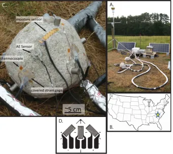
The purpose of the study is to develop protocol for a rock fracturing monitoring system for natural stone. We recognize that using natural stone potentially introduces complications in the instrumentation process, but concluded that the poten-tial payoff of success with a natural rock as opposed to a modified natural stone or a manufactured stone was worth the complication. Currently, three different test specimens have been instrumented and evaluated successfully. The test boulder described herein is a granite boulder (Fig. 1) col-lected from an active gravel bar in the Santa Ana Wash in Southern California (34◦0600400N, 117◦0601800W); hereafter referred to as “the boulder” or “the test specimen”. The boul-der is ellipsoid in shape with maximum dimensions equal to 340 mm in length, 250 mm in width, and 240 mm in height. An attempt was made to collect a boulder with as few vis-ible fractures on the surface as possvis-ible. However, there is a vertical dimple on the examined rock (Fig. 1b). The boul-der was collected from a dry wash in a semi-arid environ-ment assuming that such a clast would be episodically tum-bled in the channel, causing breaking along any major in-herited fracture, while remaining relatively dry. The boulder is a hornblende-biotite granodiorite likely from Cretaceous granodiorite of Angel Oakes (Morton and Miller, 2003). It is coarse-grained (average grain diameter 1–5 mm), nonfoli-ate, and nonporphyritic. Granite was chosen as a rock type to minimize complications due to heterogeneities such as bed-ding or foliation. The boulder was stored out in the open in a typical campus laboratory for approximately one year prior to deployment in the field.
A.
B.
“dimple”
Fig. 1. Photographs of two different views of the granite boulder selected to be the test specimen for the instrumentation campaign described in this study.
were also installed at the site to simultaneously monitor the ambient environmental conditions experienced by the boul-der. The following sections describe each component of the instrumentation and data acquisition configuration. The in-strumentation system was improved over the course of three years and three different test specimens. We describe the con-figuration in sufficient detail so that the actual installation can be duplicated by future researchers.
3 Measurement of strain
Foil strain gage selection is dependent upon the application and the ability to determine the orientation of the principle axis during a measurement. For this study, we chose a Vishay Micro-Measurements rectangular rosette consisting of three strain gages oriented 45◦ to one another. The rectangular rosette used for this project is a universal, general-purpose foil strain gage with a constantan grid that is encapsulated in polyimide. Because that rectangular rosette utilized in this project (Fig. 2d) utilizes a “planar” construction method (i.e., the three foil gages lie side by side rather than on top of
each other), the entire gage area is thinner and more flexible, which is better for curved surfaces (e.g., small boulders). Ad-ditionally, a “planar” configuration provides for better heat dissipation, more freedom in lead wire routing and attach-ment, and is available in most (if not all) gage configurations and lengths. A rosette that stacks all three gages on top of each other is best utilized when the surface area on the test specimen is limited and/or when there is a steep strain gradi-ent that exists over a short length on the test surface (Vishay Micro-Measurements, 2005).
For this field application, it was important to (1) mea-sure the strain at multiple select locations on a relatively small boulder (∼25 cm diameter), (2) minimize the sur-face area covered by the gage, and (3) ensure an excellent electrical connection capable of withstanding harsh environ-mental field conditions. The backing of the gage measured 12.7 mm by 19.3 mm, and each of the three foil gages mea-sured 3.05 mm by 6.35 mm. A∼6 mm length gage ensured that each gage would span a minimum of two individual mineral crystals, given the 5 mm maximum grain size of the boulder in this application. The authors do not recommend a smaller gage for a boulder of this size due to the diffi-culties associated with wiring small soldering tabs. A 350 resistance gage was selected to reduce the required power and the amount of heat generated. A 350resistance gage also decreases lead wire effects including circuit desensitiza-tion due to lead wire resistance and unwanted signal varia-tions caused by lead wire resistance changes with tempera-ture fluctuations.
AE sensor
moisture sensor
~5 cm
covered strain gagethermocouple AE Sensor
A.
B.
C..
D.
Fig. 2. (A) Photograph of the final instrumentation array and (B) map of the final deployment location for the boulder. (C) Close-up photo-graph of the instrumented boulder on site. (D) Diagram of strain rosettes used in this study.
attached to a flat surface to ensure there is adequate and uni-form contact between the surfaces while the adhesive cures. Because of the rounded shape, it was impractical to apply a standard weight to the gage in the same way, so each gage was covered with a thick piece of silicone rubber and truck straps were tightened over this rubber to apply an adequate, uniform pressure around the boulder.
The installation orientation of a rectangular rosette foil strain gage does not matter as long as the orientation of gage 1 on the rosette is determined with respect to a known axis. The direction of gage 1 for all eight foil strain gages was measured with respect to the north–south axis established on the boulder (further described below).
A durable environmental protection layer was applied to each gage to ensure the long-term electrical integrity of the gage in the field (Fig. 2c). To accomplish this task, a layer of masking tape was applied to the boulder to create a boundary area surrounding the gage and the head of the lead wires. At the recommendation of the manufacturer, a paintbrush was used to coat the inside area with hot wax to ensure the en-vironmental protection was able to surround the wires and fill in all tight spaces. To provide an extra layer of durability, the environmental protection was further covered in a layer
of clear, RTV silicone adhesive (Dow Corning 3140), specif-ically designed to waterproof electrical applications.
did attempt to document their orientations relative to our grid system by horizontally projecting both the grid lines and the gage 1 line while measuring the angle between them with a protractor.
The equations required to calculate principal strains from a rectangular rosette that contains three independent measure-ment grids are derived from a strain–transformation relation-ship, which expresses the normal strain in any direction on the surface of a test specimen (εθ) in terms of two principal strains (εP andεQ) and the angle (θ) from the major princi-pal axis to the direction of the specified strain. The normal strain at any angle (θ) from the major principal axis can be calculated using Eq. (1) and Mohr’s circle.
εθ =
εP +εQ
2 +
εP −εQ
2 cos(2σ ) (1) Assuming that measurement grid 1 in Fig. 2d is positionedθ degrees from the major principal axis, measurement grids 2 and 3 are positioned at θ+45◦ and θ+90◦, respectively, from the major principal axis. These angles can be substi-tuted into Eq. (1) to calculate the strain value for measure-ment grids 1, 2, and 3 as displayed in Eqs. (2)–(4) below.
ε1 = εP +εQ
2 +
εP −εQ
2 cos(2θ ), (2) ε2 =
εP +εQ
2 +
εP −εQ
2 cos(2(θ+45
◦)), (3)
ε3 =
εP +εQ
2 +
εP −εQ
2 cos(2(θ+90
◦
)) (4) Whileθ and the major and minor principal strains are un-known, the measurement grid strains (ε1,ε2, andε3) are cal-culated from the voltage measurements acquired by the data acquisition logger. Foil strain gages are resistance gages. By supplying a precise, known voltage to a resistive circuit (i.e., the foil strain gage) and measuring the return voltage, the re-sistance is calculated and then converted to engineering units of strain using the gage calibration factor, which can then be utilized in Eqs. (2)–(4). Therefore, Equations 2, 3, and 4 can be solved simultaneously to determine the three unknowns (εP,εQ, andθ). Equations (5) and (6) displayεP,εQ, andθ, respectively. It is important to note that the angle,θ, repre-sents the acute angle from the principal axis to the reference grid (clockwise rotation).
εP =
(ε1+ε3)
+ √1
2 q
(ε1−ε2)2+ (ε2−ε3)2 (5)
εQ =
(ε1+ε3)
2 −
1
√
2 q
(ε1−ε2)2+ (ε2−ε3)2 (6)
θ = 1
2 tan
−1 ε
1−2ε2+ε3 ε1−ε2
(7) It is important to note that because the selected boulder is rounded, there is notable potential error in the calcula-tions of absolute strain. The mathematics associated with
foil strain gage calculations assume the gage is attached to a flat, smooth surface that extends infinitely in all directions. Therefore, the strains calculated during this project cannot be viewed as measurements of true strain on the test specimen. However, the relative values of the magnitude and direction (tension versus compression) at each measurement location can be compared to the other gages and should provide mean-ingful information about the state of strain across the boulder surface. In order to validate that the foil strain gage measure-ments were properly acquired by the hardware and accurately manipulated by the software, data collected by the CR1000 logger using a strain gage installed on a separate surface were compared to an independent vibrating wire strain gage on the same surface (read by a Geokon GK404 readout box) dur-ing a laboratory compression test. The foil strain gage data closely matched the vibrating wire strain gage data with an R2value of 0.98.
Because strain is calculated relative to prescribed an-tecedent conditions, foil strain gage baseline readings must be measured under constant environmental conditions (at room temperature) prior to field deployment. Strain gage data were measured for all 24 gages by the data acquisition sys-tem while the test specimen was located in a laboratory en-vironment at a constant room temperature. Since mechanical and temperature induced strain will not vary under these con-trolled conditions, the average strain value for each gage was calculated, inputted into the software program, and used as a reference measurement for all strain data moving forward.
4 Measurement of surface temperature
A standard T-type thermocouple (Omega SA1XL-T-120) with a copper–constantan junction was utilized for this project (Fig. 2c). Due to the durability, repeatability, and re-sponsiveness of this temperature measurement sensor, it is widely used and accepted in a variety of engineering field studies that require measurement of surface temperature on various materials. The stated accuracy of this sensor (±1◦C) is adequate for this analysis and is capable of functioning in temperatures ranging from −200 to 350◦C. A cement adhesive (Omegabond 400) was used to attach all thermo-couples to the rock test specimen following manufacturer’s instructions.
The temperature differences that we recorded between full sun and shaded conditions ranged from 1.1 to 1.4◦C. Thus,
it was concluded that the direct radiation induced tempera-ture error on the thermocouples is relatively small and that daily highs render them only slightly warmer than the actual surface temperature.
5 Measurement of acoustic emissions
Acoustic emissions are defined as transient elastic waves generated by the rapid release of strain energy or by the sud-den redistribution of stress within a material. The majority of sources of acoustic emission activity in rock are attributed to damage-related deformation such as the initiation and prop-agation of micro-fractures, and plastic deformation (Rao et al., 1999; Lei et al., 2000; Khair, 1984). The purpose of an AE sensor (also referred to as a piezoelectric transducer) is to convert the mechanical energy carried by an elastic wave into an electrical signal. An adhesive couplant must be used to at-tach the gage while ensuring that voids do not exist between the specimen and sensor.
The frequency, sensitivity, size, and temperature capability of commercially available sensors were evaluated as part of the sensor selection process. The sustainability of the equip-ment and sensors in a natural, outdoor environequip-ment was also important for this field-based project. A moderate frequency (100–450 kHz), pre-amplified, low power consumption sen-sor (Physical Acoustics Corporation PK151) was selected with the help of the manufacturer (displayed in Fig. 2c). Physical Acoustics Corporation (PAC) equipment, sensors, and software were selected for use during this project since they were the only US based company that could provide three dimensional location capability of an acoustic emission event at that time in the planning process.
The PAC SH-II data acquisition system utilizes two soft-ware programs for monitoring and analysis. The SHClient software controls all primary communications with the AE sensors on the rock during the calibration process and during the data collection period. It is also used to set up all initial configurations for the hardware. It is important to distinguish the difference between an AE “hit” and an AE “event”. If the elastic wave measurement exceeds a pre-defined thresh-old value and is measured by one of the pre-amplified sen-sors attached to the specimen, data will be recorded and re-ferred to as an acoustic emission “hit”. If the same wave is registered by at least four sensors on the specimen, it is referred to as an AE “event”. The four sensor minimum configuration was specified by the manufacturer for the cal-culation of location in a three dimensional domain. It also serves as a conservative method for distinguishing significant AE-producing phenomena affecting the rock. The higher the number of acoustic emission hits, the higher the associated physical damage to the rock (i.e., fracture initiation and prop-agation; e.g., Huang et al., 1998). Furthermore “burst” types
of AE waveforms that have been observed in this study are associated with fracture initiation and propagation (Pollock, 1989). Pre-deployment observations determined that effects from small impacts including insects landing on the rock or small sand grains hitting the rock might register hits on one or two sensors. Therefore, rock damaging AE events are consid-ered to be associated with AE events caused by activity from four sensors simultaneously measuring the same activity. It should be noted that establishing direct correlations between AE data and actual rock damage is a complex process (e.g., Huang et al., 1998). There is no direct way to distinguish, for example, crack initiation from crack propagation or to make a direct correlation between event signal and length of rup-ture. It is possible in some cases to determine the mode of cracking, but such an analysis was beyond the scope of this study.
While four sensors were the established minimum, six sen-sors were utilized for all future AE sensor installations, but there are several key location criteria that must be met to accurately quantify a three-dimensional location using AE data. It is important that (1) the locations of the sensors be arranged in a pattern that ensures no four sensors are on the same plane, (2) every combination of three AE sensors forms a triangular plane, and (3) multiple planes are as orthogonal to each other as possible. Meeting these criteria while estab-lishing the installation locations of the sensors on any test specimen is not trivial and requires trial and error testing.
The field data collected by the SHClient software is then imported into the AEwin software to calculate the three-dimensional source location of an AE wave. In general, AE source localization is determined using an arrival time that is calculated using a trial or guessed location that was derived using arrival times of individual sensors, and a user-defined velocity (see below). The guessed location is then corrected using differences between measured and calculated arrival times. The calculated arrival time can be written as
tic =t(xi,yi,zi,x0,y0,z0)+t0.
5.1 Determination of wave velocity
In general, the wave velocity material property is determined by a calibration process that involves inducing a wave on the material and calculating how fast it takes an AE sensor at-tached to the material to receive that signal, knowing the dis-tance that the wave traveled. As a first step in the iterative calibration process, two rectangular calibration blocks were specially cut from two similar but not identical rock materi-als (two different granites) so that simple, square geometry (origin located at one corner of the calibration block) could be used to determine distances between each AE sensor in-stalled on the calibration specimen. For a three-dimensional block or boulder, point location (x,y, andzcoordinates in a three dimensional domain) is required. The software specifi-cations require a minimum of four sensors to provide “point” location capability, but the use of additional sensors is rec-ommended to increase success and cover wide surface areas. It also depends upon the size of the test specimen, and this process can only be validated through trial and error.
With the sensors in position on the calibration block, an AE event was simulated using a pencil lead break (PLB) test in accordance with the American Society for Testing and Ma-terials standard specification (ASTM E 976). Multiple PLB tests were performed adjacent to individual sensors so that the distance between that sensor and the PLB was zero. As such, the timing of the first return of the AE represents the timing of the PLB itself. Thus the travel time of the PLB event to all 5 remaining sensors could be determined by the AE system. Using the xi, yi, and zi coordinates of each sen-sor (i), the known location (xplb, yplb, zplb)of the PLB on the calibration block, and the time recorded (t i) by the AE data acquisition system that it took each sensor to register the PLB activity induced on the material, the wave velocity of the granite block and be calculated:
Vi =(sqrt
xi −xplb2+ yi −yplb2+ yi −yplb2
/ti.
This process was repeated at multiple locations and a statis-tical analysis was performed to determine the average wave velocity for this material as a starting point. For the first cal-ibration block, the average wave velocity was determined to be 5353.501 m s−1. To validate this value, it was inputted in the software, and used to verify the location of all subsequent PLB tests. This validation exercise was performed 10 times in seven different PLB locations on the surface of the rock. The average source location calculated by AEwin was within 10.1 mm on average (standard deviation equal to 2.4 mm) of the actual PLB location on the calibration block.
Subsequently, the same process was repeated for a second, different calibration block composed of the same granite as our final test specimen. These block tests resulted in an av-erage wave velocity equal to 2293.2 m s−1. Ten PLB valida-tions tests were performed for this block in six different loca-tions, and the average source location calculated by AEwin
was within 11.3 mm on average (standard deviation equal to 4.8 mm) of the actual PLB location on the calibration block. Noting the difference in wave velocity values for two cali-bration blocks that were cut from similar parent rock mate-rial (two different granites), it was determined that it would be beneficial to determine wave velocity directly on the test specimen itself. The authors felt that any accuracy lost using a dimensionally complex specimen was outweighed by the benefit of making the measurement directly on the specimen. To facilitate the consistent and accurate determination of the coordinates on a spherical test specimen, a three sided corner box was constructed, the boulder was placed inside, and thex,y, andzcoordinates were easily measured from the sides of the box to the point location of the PLB test. The origin of the coordinate system (0, 0, 0) was located at the in-tersection of the three sides of the corner box. In subsequent test specimens, high resolution lidar scans were utilized to obtain more accurate surface measurements.
PLB tests were performed at various locations on the boul-der, and the measured versus actual coordinates of each PLB test were compared. Initially, acceptable readings were ac-quired using the wave velocity from the second calibration block. In one area on the rock (near the location of the dim-ple displayed on Fig. 1b), however, the velocity did not give accurate results. Because that portion of the rock did not have sensors in the vicinity, the AEwin software was unable to ac-curately locate AE sources in this area. As part of the itera-tive, trial and error process, one sensor was moved from the bottom of the rock to the top of the dimple. The validation exercise was repeated and the difference between the mea-sured coordinates and actual coordinates of the PLB test was reduced.
As a last step to further refine the 2 293 201 mm s−1wave velocity, this value was systematically varied in magnitude as a software input (2 200 000; 2 400 000; 2 600 000; and 2 800 000 mm s−1) until the coordinates more closely con-verged. The best results were achieved on the boulder using an average wave velocity equal to 2 400 000 mm s−1. This value was inputted into the software, the validation exercise was performed 10 times in five different locations, and the average measured location calculated by AEwin was within 24.8 mm on average (standard deviation equal to 9.6 mm) of the actual PLB location determined using thex,y,z coordi-nate system established.
the weight of each senor from overcoming the strength of the adhesive.
5.2 Measurement of surface moisture
A Campbell Scientific 237F wetness sensing grid (Fig. 2c) was used to evaluate the surface moisture on the boulder in the field. This sensor is designed to measure moisture on the surface of plant materials. It consists of a flexible polyamide film circuit (14 mm by 90 mm) with interlacing gold-plated copper fingers. Any condensation or rain on the sensor will lower the resistance between the copper fingers (spaced 0.25 mm apart to ensure a resistance change due to fine droplets). This sensor was attached to the top of the test specimen and wire solders were protected using the same M-Bond AE10 adhesive and RTV silicone that were used for the foil strain gages.
The levels of resistance as a function of moisture were evaluated in a controlled laboratory environment. Upon care-ful misting with water, sensor resistance ranged from>0 to 200 k even with single droplets of water. Therefore, any reading higher than 200 was considered dry and any reading less than or equal to 200 is considered to indicate the pres-ence of moisture.
6 Measurement of environmental and soil conditions
In order to monitor the micro-climate at the field site, a stan-dard Campbell Scientific weather station capable of measur-ing ambient temperature, relative humidity, wind speed, wind direction, barometric pressure, insolation and precipitation (to 0.1 mm) was installed on site.
Although the boulder was not embedded in the ground dur-ing this study, it was anticipated that soil moisture might af-fect ground surface temperature, possibly impacting the bot-tom temperature of the boulder. A CS616 water content re-flectometer was installed to measure the volumetric water content of soil using time-domain measurement methods that are sensitive to the dielectric permittivity of any material. The calibration curve supplied by the manufacturer was verified in a controlled laboratory environment.
7 Data acquisition configuration
A Campbell Scientific CR1000 served as the logger for all instrumentation on the surface of the rock and adjacent to the test specimen (including the soil probe and weather station) with the exception of the AE sensors. The logger monitored the 24 strain gages via two Campbell Scientific AM16/32, 16-channel multiplexers, and it monitored the eight thermo-couples via a single AM 25T, 25-channel multiplexer. The soil probe and weather station sensors were connected di-rectly to the logger.
The main components of the PAC SH-II logger included the CPU board and two four-channel modules, which con-tain the analog circuitry for the system and process the ana-log input signals from the sensors with the use of filters and analog–digital converters. Up to eight AE sensors can be monitored using this configuration.
Both systems were enclosed in water-tight enclosures for this field application and all data was downloaded using a CDMA cellular modem that interfaced with the data logger software. McKay et al. (2009) and Hall and André (2003) noted that>1 measurement per minute temporal resolution of data may provide key insights into fracturing processes and the data acquisition system described herein was able to achieve that sampling frequency.
While it was possible to connect directly to both systems using either a serial cable (for the CR1000) or an Ethernet cable (for the SH-II), both systems were routinely down-loaded using a CDMA technology cell-phone connection. The system was powered by two 115 W solar panels (Fig. 2) regulated by a Morningstar PS regulator/controller. Back-up power was provided by three additional 12 V, 116 Ah batter-ies to ensure continuous power.
8 Field deployment process
The boulder was deployed to the middle of a cow pasture with full sun exposure located on a drainage divide in Bel-mont, North Carolina (Fig. 2b). For our application, it was important to locate an open site without shade from trees or structures. Additionally, it was important that the site did not have power lines in the vicinity that would generate “noise” in the AE signals. Before deployment, it was important to identify any sources of noise on site that may cause error in the AE data due to the sensitivity of this measurement. To determine potential sources of noise on site, raw data was collected continuously for approximately one hour using the AE data acquisition system and there were no hits or events during this time period. Previous rock specimens installed on campus (on roof tops or closer to mechanical equipment near buildings) and off campus in residential areas (closer to power line sources) clearly showed noise issues in the data during an equivalent noise check exercise.
mast for the weather station was constructed to the northwest of the rock to ensure minimum shading.
9 Preliminary results and discussion
In the course of this research, three boulders have been de-ployed including this one (Garbini, 2009; Eppes et al., 2012). All three boulders show similar spatial and temporal patterns in AE events, surface conditions, and microclimate. These similarities strongly suggest that the results have general va-lidity instead of being specific to an individual boulder. The preliminary data presented herein demonstrates the data va-lidity and showcases the overall range of spatial and temporal analyses that the data set allows.
The boulder described in this paper was monitored for 11 months (20 June 2010 through 18 May 2011) in the field. A preliminary analysis of that data set for the months of June through September 2010 is presented. During this time pe-riod, we recorded data for 92 days. Loss of data days was due to periodic power failures and a site disturbance. For these 92 days when data was complete, 11 607 acoustic emission events (signal simultaneously detected by at least four trans-ducers) and 638 960 hits (signal detected by 1–3 transtrans-ducers) were recorded by the AE data acquisition system. A linear re-gression correlating hit and event data yields anR2of 0.41 with a Pearson’sp value of<0.05. The relatively low R2 is due to the fact that there are many days when there are hits but no events in the data set. If those days are removed, then theR2rises to 0.69. Overall, there is relatively strong relationship between the time that hits and events occur, but there are a significant number of instances when hits occur unassociated with events. We interpret these results to mean that our four hit per event threshold represents a conserva-tive yet strong proxy for the total amount of fracture damage experienced by the rock. Although it is beyond the scope of this paper, AE Win software also calculates other waveform data associated with each event. Future analyses will further differentiate damage-causing events as a function of their en-ergy. The remainder of this discussion will focus on overall amounts, timing and locations of events.
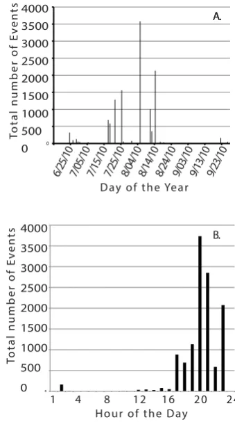
The 11 607 events occurred within 367 different time stamps (each representing a unique 60 s time interval) dur-ing 36 days out of 92 on record. AE events were typically recorded in temporal clusters (multiple events over the course of a few minutes time on a few specific days). For exam-ple, more than 95 % of the events occurred during only 12 % (11 days) of the time period. There were also patterns in the overall daily timing of events. The vast majority of all events (96 %) were recorded during the late afternoon and evening hours (between 16:00 and 23:00 LT – Eastern Stan-dard Time). No events occurred between 03:00 and 09:00 LT (Fig. 3). Both field measurements of fracture orientations (McFadden et al., 2005; Eppes et al., 2010; Fig. 4) and nu-merical modeling of stress in a rounded boulder exposed to
0
1 2 3 4 5 6 7 8 9101112131415161718192021222324
4000 3500 3000 2500 2000 1500 1000 500 0
1 4 8 12 16 20 24 Hour of the Day
To
tal number of E
vents
0
4000 3500 3000 2500 2000 1500 1000 500 0
Day of the Year
To
tal number of E
vents
6/25/10 7/05/10 7/15/10 7/25/10 8/04/10 8/14/10 8/24/10 9/03/10 9/13/10 9/23/10 A. A.
B.
Fig. 3. Histogram of numbers of events for the time period of June– September 2010 as a function of (A) date and (B) hour of the day.
diurnal temperature changes (Shi, 2011) predict that morning might be a prominent time for rock fracturing, but these data indicate that morning is characterized by few, if any, fracture events. Thus, even this simple temporal analysis of the AE data set demonstrates the robustness of the data and its high potential for contributions to physical weathering research.
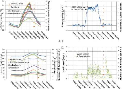
Rock surface and environmental data also provide key in-sights into the conditions under which fracturing occurs. Fig-ure 5 displays four graphs, which depict temperatFig-ure, temper-ature difference across the surface of the rock, select weather conditions (wind speed), and maximum principle strain as a function of time for a typical day in which events occur (26 July 2010). Additionally, the number of AE events oc-curring each minute of this day is depicted on the secondary axis of each graph. The graphs in Fig. 5 are representative of a typical suite of graphs automatically generated for each day of data that is collected. In general, the patterns visible in this figure are notably repeated throughout this data set and were also observed during event clusters that occurred during the monitoring periods associated with the other two test speci-mens previously mentioned. A more detailed comparison of all data sets will be completed for future publications.
284 K. Warren et al.: Automated field detection of rock fracturing, microclimate, and diurnal rock temperature
(a) (b)
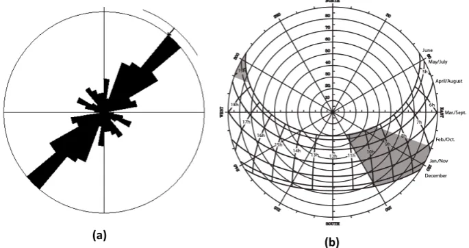
Fig. 4. Modified from Eppes et al. (2010). A. Rose diagram of measured crack orientations from 101 rocks in the Gobi Desert. Arc represents 2σ mean resultant direction of data (40◦northeast). B. Sunpath solar path chart for the Gobi field site. Modified from a chart created through the University of Oregon Solar Radiation Monitoring Laboratory website. Shaded areas represent instances when the sun would be at a 90◦angle from average crack angle of 40◦. This type of field data is exemplary of this and other studies that show that rock cracks exhibit preferred orientations (e.g., Eppes et al., 2010; McFadden et al., 2005). If cracks form perpendicular to the direction of heating and cooling, then these preferred orientations suggest that cracks form due to stresses that arise in the morning (Eppes et al., 2010).
peak early afternoon, and then decrease continuously into the evening. The timing and/or magnitude of diurnal temperature changes that we observe throughout the data set are gener-ally consistent with other shorter-term studies of rock surface temperatures (e.g., McKay et al., 2009; Viles, 2005; Hall and André, 2003). Surface temperatures on the test specimen are consistently higher than ambient temperature, and all tem-peratures appear to be rapidly influenced by cloudiness (il-lustrated in insolation data), wind speed, and direction. The thermocouple on the rock with the highest temperature and the thermocouple with the lowest temperature recorded each minute are used to determine the maximum range in surface temperature across the boulder’s surface (Fig. 5b). In gen-eral, the largest temperature range across the rock surface (almost 20◦C) is between the south and/or top sides of the boulder and the bottom of the boulder. On any given day, this range is relatively low until all temperatures begin to increase through the early morning in conjunction with the absolute surface and air temperature. Because this data set enables the determination of spatial and temporal variability of the tem-perature characteristics of the rock over an entire year, this surface temperature data set is an unprecedented opportunity to address the frequency, duration and/or magnitude of condi-tions that are often hypothesized to lead to fracture. Hypothe-ses related to procesHypothe-ses such as freeze–thaw (e.g., the amount of time a rock is in the proposed−4 to−15◦C range thought
to be ideal for fracturing by sustained freezing temperatures; Walder and Hallet, 1985; Hallet et al., 1991) and/or ther-mal shock (e.g., the hypothesized 2◦C min−1 threshold of-ten cited for thermal shock fracturing; Richter and Simmons, 1974) can be directly tested with the data set.
Fig. 5. Graphs of total numbers of events per minute (each orange box represents data for an individual minute) for a single day (26 July 2010) along with concurrent per minute. (A) Rock surface and ambient temperature, (B) temperature difference between the hottest and coldest thermocouple on the rock, (C) calculated maximum principal strain for all 8 strain gages and ambient temperature, and (D) wind speed measured adjacent to the rock.
The AE events recorded on 26 July occur at approximately 18:00 LT as surface and air temperatures are in an overall state of cooling. Additionally, at the time that these events occur, there is a notable, small increase in temperature range (the difference between coolest and warmest surface temper-ature). The coincidence of AE events with a secondary, late-afternoon or early evening spike in rock surface temperature range was observed frequently for this boulder as well as for other boulders (Garbini, 2009; Eppes et al., 2012). The drop in wind speed (Fig. 5c) that occurs during this time period likely explains the second spike in the temperature range, where the loss of heat advection by wind would have caused the upper surface of the rock to warm up again. On most other days with major event clusters, similar abrupt changes (typi-cally increases) in rain or wind are observed coincident with the timing of the events. Changes such as these in microcli-mate have been shown or hypothesized by others to lead to very rapid rock surface temperature fluctuations (McFadden et al., 2005; Molaro and McKay, 2010). This data set will
enable the characterization of those weather conditions that lead to rapid change in rock surface conditions and help de-fine a suite of conditions that correlate most strongly with AE events. Using long-term climate records, the potential past frequency of such conditions can then be determined. Such comparisons will allow us to (1) determine if the envi-ronmental conditions that are associated with rock fracturing are extreme compared to long-term climate, (2) use the fre-quency of such climate conditions in the past to infer future rates of rock fracturing relative to the period of observation, and (3) consider rates of physical weathering as a function of past climates that may have had higher prevalence of such conditions.
B.
West East A.
distance (mm)
distanc
e (mm)
top
bottom
South Northdistance (mm)
distanc
e (mm)
top
bottom
West East north
south
distanc
e (mm)
distance (mm) C.
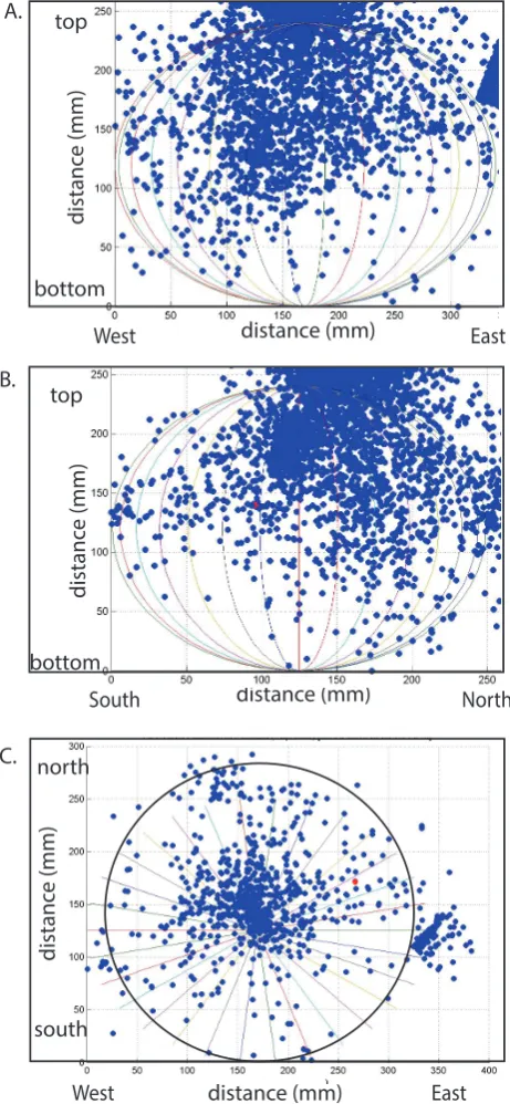
Fig. 6. Graphical representation of the location of events as calcu-lated by AEwin software for (A) a west to east side view of the test specimen, (B) a south to north side view of the test specimen and (C) a top-down view of the test specimen. In all figures, the ellipsoid shape is an approximate location of the surface of the rock based on its maximum dimensions. The events that are plotted are those that fall within 5 cm of the ellipsoid shape (5051 events).
visualize the locations with respect to our boulder, a three-dimensional ellipsoid approximation of the exterior shell of the boulder was generated within MATLAB using the boul-der’s dimensions (length, width, and height). This ellipsoid was then plotted along with the calculated locations of events in an attempt to identify spatial patterns of boulder damage.
In order to focus on accurately localized events, events that fall within a 5 cm margin of a generalized ellipsoid the shape and size of the test specimen are targeted for analy-sis (Fig. 6). Although a relatively large number of events (∼50 %) fall outside of this region, broad clouds of data similar to this data set are the norm when localizing large amounts of AE data using automated software (e.g., Grosse and Ohtsu, 2008). In particular, a complex test specimen (i.e., natural rock) with irregular boundaries and an inhomoge-neous structure causes reflections and scattered waves that interfere with the signal and the localization effort. Never-theless, it is generally accepted that the overall density of AE localizations can be used as a reliable indicator of the location of a region of high AE activity/source within a spec-imen, because correct locations will be concentrated in ac-tual areas of fracture within the rock (e.g., Grosse and Ohtsu, 2008). Furthermore, the timing and numbers of individual AE events associated with miss-locations have been shown to represent valid emissions due to rock damage (e.g., Grosse and Ohtsu, 2008); they are just not properly localized. Thus, overall, (1) the number of AE events represents a satisfactory proxy for relative amounts of fracture initiation and propa-gation and (2) the densest clouds of location data that fall within the ellipsoid can provide meaningful insight into gen-eral fracture locations.
A preliminary visual inspection of this data set shows that the majority of the events are located in the upper hemisphere of the boulder, with some possible clustering evident in the center of the boulder. There is notably no visible clustering in the vicinity of the “dimple” on the northwest-facing side of the boulder. In the future, we hope to compare this location data with field data of macro-crack locations (Eppes et al., 2011) and with numerical models of the locations of maxi-mum stress accrued in a diurnally heated boulder (Hallet et al., 2012). Future 4-D spatial/temporal statistical analysis of the data will also allow us to determine if events forming un-der varying temperature and/or strain conditions are initiated in different locations within the test specimen.
10 Conclusions
Based on the data that has been collected on this test speci-men (in addition to previous and ongoing test specispeci-mens), the AE events represent mechanical deformation in the test boul-der that is due to fracturing commonly experienced by gran-ite boulders exposed to diurnal conditions. While the calcu-lated locations of these AE events have a relatively high mar-gin of spatial error, relevant information from these data has been collected and will be utilized to facilitate the ongoing spatial analysis effort. At a minimum, it has been shown that fracturing of the boulder can be monitored simultaneously with the concurrent surface and ambient conditions before, during, and after the time of fracturing with high spatial and temporal resolution.
Since the completion of the work described herein, a third test specimen was instrumented and deployed during the summer of 2011 for a two year monitoring period in New Mexico to monitor conditions in a desert environment over a longer time duration. These data have also been uti-lized by participating colleagues (e.g., Hallet et al., 2012) to provide accurate inputs and testing of numerical models of stress states of boulders exposed to natural diurnal condi-tions. Macrocrack field data continues to be collected around the globe (e.g., Eppes et al., 2011). The combination of an extensive instrumentation monitoring program like this one in conjunction with field data and numerical modeling rep-resents an unequivocal step to deconvolving the mechanical processes that lead to non-tectonic rock fracture for rocks that are subaerially exposed on Earth’s surface.
Acknowledgements. This research was funded by two National Science Foundation (NSF) awards (0844335 and EAR-0705277). The authors would like to thank Jim Conrad and Andrew Willis of UNC Charlotte for their support throughout this project. We would also like to thank the Redlair Research Preserve for the use of their land and Doug Shafer for use of his property during a previous field study, as well as Bernard Hallet, Peter Mackenzie and Les McFadden for fruitful discussions and field visits to our deployed rocks.
Edited by: L. Eppelbaum
References
Amit, R., Gerson, R., and Yaalon, D. H.: Stages and rate of the gravel shattering process by salts in desert Reg soils, Geoderma, 57, 295–324, 1993.
Blackwelder, E. B.: The insolation hypothesis of rock weathering, Am. J. Sci., 226, 1324–1400, 1933.
Eberhardt, E., Stead, D., Stimpson, B., and Read, R. S.: Identifying fracture initiation and propagation thresholds in brittle rock, Can. Geotech. J., 35, 222–233, 1998.
Eppes, M. C., McFadden, L., Wegmann, K., and Scuderi, L.: Frac-tures in desert pavement rocks: further insights into mechanical weathering by directional solar heating, Geomorphology, 123, 97–108, 2010.
Eppes, M. C., Aldred, J., Aquino, K., Deal, R., Garbini, J., Swami, S., Tuttle, Al., and Xanthos, G.: Documentation of preferential orientations of cracks in boulder fields of temperate climates: Further evidence for the influence of directional insolation in physical weathering, vol. 43, Geological Society of America An-nual Meeting, October 2011, Minneapolis, MN, Abstracts with Program, p. 252, 2011.
Eppes, M. C., Warren, K., Hinson, E., and Dash, L.:. Physical weathering by insolation: comparison of year long, per-minute observation so temperature, strain and cracking in granite boul-ders in a temperate pasture and semiarid desert, North Carolina and New Mexico, Vol. 44, Geological Society of America Ab-stracts with Programs, p. 145, 2012.
Garbini, J.: Instrumentation and analysis of the diurnal processes af-fecting a natural boulder exposed to a natural environment, UNC Charlotte Thesis, Charlotte, USA, p. 148, 2009.
Girard, L., Beutel, J., Gruber, S., Hunziker, J., Lim, R., and We-ber, S.: A custom acoustic emission monitoring system for harsh environments: application to freezing-induced damage in alpine rock walls, Geosci. Instrum. Method. Data Syst., 1, 155–167, doi:10.5194/gi-1-155-2012, 2012.
Grosse, C. and Ohtsu, M.: Acoustic Emission Testing, in: Technol-ogy & Engineering, Springer Verlag Berlin Heidelberg Germany, 1–396, 2008.
Hall, K.: The role of thermal stress fatigue in the breakdown of rock in cold regions, Geomorphology, 31, 47–63, 1999.
Hall, K. and André, M. F.: Rock thermal data at the grain scale: ap-plicability to granular disintegration in cold environments, Earth Surf. Proc. Land., 28, 823–836, 2003.
Hall, K. and Hall, A.: Weathering by wetting and drying: some ex-perimental results, Earth Surf. Proc. Land., 21, 365–376, 1996. Hallet, B., Walder, J., and Stubbs, C. W.: Weathering by
segrega-tion ice growth in microfractures at sustained sub-zero temper-atures: verification from an experimental study using acoustic emissions, Permafrost Periglac., 2, 283–300, 1991.
Hallet, B., Mackenzie-Helnwein, P., Shi, J., and Eppes, M.: Are thermal stresses in rocks exposed to the sun sufficient to break them? Yes, Vol. 44, No. 7, Geological Society of America Ab-stracts with Programs, p. 145, 2012.
Huang, M., Jiang, L., Liaw, P., Brooks, C., Seeley, R., and Klarstrom, D.: Using Acoustic Emission in Fatigue and Frac-ture Materials Research, J. Mech., 50, http://www.tms.org/ pubs/journals/JOM/9811/Huang/Huang-9811.html (last access: November 2013), 1998.
Khair, A.: Acoustic emission pattern; an indicator of mode of failure in geologic materials as affected by their natural imperfections, Acoustic Emission/Microseismic Activity in Geologic Structures and Materials, proceedings of the third conference 1981, Univer-sity Park PA, USA, 45–66, 1984.
Lei, X., Kusunose, K., Rao, M., Nishizawa, O., and Satoh, T.: Quasi-static fault growth and fracturing in homogeneous brittle rock under triaxial compression using acoustic emission moni-toring, J. Geophys. Res., 105, 6127–6139, 2000.
McFadden, L. D., Eppes, M. C., Gillespie, A. R., and Hallet, B.: Physical weathering in arid landscapes due to diurnal variation in the direction of solar heating, Geol. Soc. Am. Bull., 110, 161– 173, 2005.
McKay, C. P., Molaro, J. L., and Marinova, M. M.: High-frequency rock temperature data from hyper-arid desert environments in the Atacama and the Antarctic Dry Valleys and implications for rock weathering, Geomorphology, 110, 182–187, 2009.
Molaro, J. L. and McKay, C. P.: Processes controlling rapid tem-perature variations on rock surfaces, Earth Surf. Proc. Land., 35, 501–507, 2010.
Moores, J. E., Pelletier, J. T., and Smith, P. H.: Fracture propagation by differential insolation on desert surface clasts, Geomorphol-ogy, 102, 472–481, 2008.
Morton, D. M. and Miller, F. K.: Preliminary Geologic Map of the San Bernardino 300×600quadrangle, California, US Geological Survey Open-File report 03-293, US Geological Survey, Menlo Park, California, 2003.
Nicholson, D. T.: Pore properties as indicators of breakdown mech-anisms in experimentally weathered limestones, Earth Surf. Proc. Land., 26, 819–838, 2001.
Pollock, A. A.: Acoustic Emission Inspection, Metals Handbook, 9th Edn., Vol. 17, ASME International, Ohio, USA, 278–294, 1989.
Rao, N., Murthy, G., and Raju, N.: Characterization of micro and macro-fractures in rocks by acoustic emission, ASTM Special Technical Publication 1353, American Society for Testing and Materials, West Conshohocken, PA, 141–155, 1999.
Richter, D. and Simmons, G.: Thermal expansion behavior of ig-neous rocks, Int. J. Rock Mech., 11, 403–411, 1974.
Shi, J.: Study of Thermal Stresses in Rocks Due to Diurnal Solar Exposure, MS Thesis, University of Washingtion, Washington, 1–103, 2011.
Tanigawa, Y. and Takeuti, Y.: Three-dimensional thermoelastic treatment in a spherical region and its application to solid sphere due to rotating heat source, Z. Angew. Math. Mech., 63, 317– 324, 1983.
Turkington, A.: Stone Decay in the Architectural Environment, Ge-ological Society of America Special Publication 390, GeGe-ological Society of America, Boulder, CO, USA, p. 62, 2005.
Viles, H. A.: Microclimate and weathering in the central Namib Desert, Geomorphology, 67, 189–209, 2005.
Viles, H. A. and Goudie, A. S.: Rapid salt weathering in the coastal Namib Desert: Implications for landscape development, Geo-morphology, 85, 49–62, 2007.
Vishay Micro-Measurements: Strain gage installations with M-Bond 200 Adhesive, Instruction Bulletin, B-127-14, 1–4, 2005. Walder, J. and Hallet, B.: A theoretical model of the fracture of rock
during freezing, Geol. Soc. Am. Bull., 96, 336–346, 1985. Wegmann, M. and Gudmundsson, G. H.: Thermally induced