https://doi.org/10.5194/gmd-12-4061-2019 © Author(s) 2019. This work is distributed under the Creative Commons Attribution 4.0 License.
Beo v1.0: numerical model of heat flow and low-temperature
thermochronology in hydrothermal systems
Elco Luijendijk
Geoscience Centre, University of Göttingen, Goldschmidtstraße 3, 37077, Göttingen, Germany Correspondence:Elco Luijendijk (elco.luijendijk@geo.uni-goettingen.de)
Received: 28 December 2018 – Discussion started: 4 February 2019
Revised: 3 August 2019 – Accepted: 6 August 2019 – Published: 20 September 2019
Abstract. Low-temperature thermochronology can provide records of the thermal history of the upper crust and can be a valuable tool to quantify the history of hydrothermal sys-tems. However, existing model codes of heat flow around hydrothermal systems do not include low-temperature ther-mochronometer age predictions. Here I present a new model code that simulates thermal history around hydrothermal sys-tems on geological timescales. The modelled thermal his-tories are used to calculate apatite(U–Th)/He (AHe) ages, which is a thermochronometer that is sensitive to tempera-tures up to 70◦C. The modelled AHe ages can be compared to measured values in surface outcrops or borehole samples to quantify the history of hydrothermal activity. Heat flux at the land surface is based on equations of latent and sensi-ble heat flux, which allows more realistic land surface and spring temperatures than models that use simplified bound-ary conditions. Instead of simulating fully coupled fluid and heat flow, the code only simulates advective and conductive heat flow, with the rate of advective fluid flux specified by the user. This relatively simple setup is computationally effi-cient and allows running larger numbers of models to quan-tify model sensitivity and uncertainty. Example case studies demonstrate the sensitivity of hot spring temperatures to the depth, width and angle of permeable fault zones, and the ef-fect of hydrothermal activity on AHe ages in surface outcrops and at depth.
1 Introduction
The interpretation of thermochronological data relies on as-sumptions or models of the Earth’s temperature field (Demp-ster and Persano, 2006). Thermal model codes that are used to interpret thermochronological data can take into ac-count many processes that influence the temperatures in the Earth’s crust on geological timescales, such as heat conduc-tion, advection caused by the movement of faults blocks or changes in topography (Braun et al., 2012). However, these models do not include the thermal effects of groundwater flow, despite indications that groundwater flow often influ-ences temperatures in the upper crust and thermochrono-logical datasets (Ehlers, 2005; Ferguson and Grasby, 2011). A model study by Whipp and Ehlers (2007) forms an ex-ception and demonstrated that diffuse topography-driven groundwater flow can strongly affect low-temperature ther-mochronometers in mountain belts.
ap-atite fission track ages around the Carlin gold deposit and ages predicted by numerical models, and Luijendijk (2012), who combined an advective and conductive heat flow model, which was a precursor to the model code presented here, to model heat flow and apatite fission track ages around a hy-drothermally active normal fault.
While coupled fluid and heat flow models can provide re-alistic reconstructions of the thermal history of hydrother-mal systems, they are also relatively computationally ex-pensive, which may limit the possibility to explore the re-sponse of these systems to different parameters. Heat flow data or thermochronology data are frequently scarce and rel-atively uncertain. These data can often be explained by a number of different parameter combinations of for instance the age, duration and flow rates of hydrothermal systems. Here I present a new advective–conductive heat flow code, Beo, that can be used to model heat flow and apatite (U– Th)/He thermochronometer ages around hydrothermal sys-tems over geological timescales. In contrast to coupled fluid and heat flow models, fluid flux is prescribed and is there-fore not a function of the driving forces of fluid flow and permeability of the subsurface. This makes the code rela-tively computationally efficient and enables running larger numbers of model experiments with variable parameters. In contrast to inverse thermal models such as HeFTy (Ketcham et al., 2007) and QTQt (Gallagher, 2012) which reconstruct thermal histories of one or more samples, Beo models 2-D temperature fields over time, which can be compared to mul-tiple low-temperature thermochronology samples and which allows testing different hypotheses for the history and char-acteristics of hydrothermal activity.
2 Model development
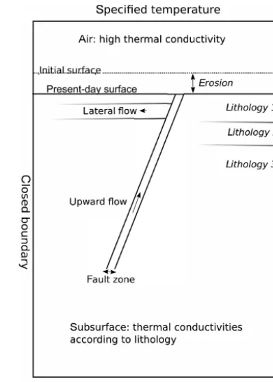
Beo was designed to model heat flow in and around a single main fluid conduit. A typical model setup is shown in Fig. 1. The model domain contains a main fluid conduit, which rep-resents permeable fault zone. The main conduit is attached to one or more horizontal fluid conduits that can be used to model lateral flow in and out of permeable formations that for instance represent alluvial sediments or permeable fractured rocks.
The following sections describe the equations used by Beo to model subsurface and surface heat flux and the apatite(U– Th)/He thermochronometer in hydrothermal systems. 2.1 Advective and conductive heat flow
The heat flow equation used by Beo to model conductive and advective heat flow in the subsurface is given by
ρbcb
∂T
∂t = ∇K∇T−ρfcfq∇T , (1) in whichT is temperature (K),tis time (s),cis heat capacity (J kg−1K−1),ρis density (kg m−3),Kis thermal
conductiv-Figure 1.Conceptual model setup. The upper and lower boundary conditions were assigned a specified temperature according to the average annual air temperature and the regional geothermal gradi-ent. No heat flow is allowed over the left- and right-hand model boundary. Fluid flows upwards along a single fault zone, part of the flux contributes to lateral flow in one or more aquifers that are con-nected to the fault. The remaining fluid discharges at the surface. Heat transfer between the surface and the atmosphere is modelled as a conductive heat flow, with a variable thermal conductivity based on equations for sensible and latent heat flux. Heat transfer in the subsurface is determined by the specific thermal conductivities of the local lithologies. The land surface is lowered over time to ac-count for erosion.
ity (W m−1K−1) andqis fluid flux (m s−1). Subscripts b and f denote properties of the bulk material and the pore fluid, respectively. Beo solves the implicit form of the heat flow equation by discretization of the derivative ofT over time:
−∇1t K∇Tt+1+1t ρfcfq∇Tt+1+ρbcbTt+1=ρbcbTt, (2)
(Geuzaine and Remacle, 2009) using a Python interface in-cluded in Escript. The discretized heat flow equation was solved using the generalized minimal residual method (GM-RES) (Saad and Schultz, 1986).
2.2 Land surface heat flux
Typical thermal boundary conditions for subsurface heat and fluid flow models are either a specified temperature or a spec-ified heat flux at the top model boundary, which is usually chosen as the land surface. However, in transient hydrother-mal systems it is difficult to simulate realistic temperature using these boundary conditions, especially in cases where fluid discharges at the surface. Assigning a specified temper-ature or heat flux would require knowledge of the change in fluid temperatures over time, which is only rarely available.
Temperatures at the land surface are predominantly deter-mined by latent and sensible heat flux (Bateni and Entekhabi, 2012). Beo uses an approach that is to my knowledge new in hydrothermal model codes, and it models the heat flux in a layer of air overlying the land surface. The top boundary of the model domain is located several metres in the air, and it is assigned a specified temperature that reflects the average annual air temperature. Latent and sensible heat flux from the land surface are approximated by assigning an artificially high value of thermal conductivity to the layer of air. The thermal conductivity of the air layer is calculated using equa-tions for latent and sensible heat flux described below.
The motivation for including the series of equations below in the model code is to simulate realistic land surface and spring temperatures in transient models. Note that the im-plementation does not add high computational demands; the equations are evaluated for land surface nodes only. In con-trast to the heat flow equations in Sect. 2.1, these equations can be solved directly without numerical methods.
Following Bateni and Entekhabi (2012) the sensible heat flux at the land surface is given by
H=ρca
ra
(Ta−Ts), (3)
where H is the sensible heat flux (W m−2) ρ is density (kg m−3),cais the specific heat of air (J kg−1K−1),rais the
aerodynamic resistance (s m−1),Tais the air temperature at
a reference level (◦C) andT
sis the surface temperature (◦C).
This expression can be combined with Fourier’s law: q=Ks
1T
1z, (4)
where q is heat flux (W m−2), K is thermal conductivity (W m−1K−1) and1T =(T
a−Ts)(K). Combining Eqs. (3)
and (4) and equalling H andq yields an expression for the effective thermal conductivity (Ks) between the surface and
the reference levelz: Ks=
ρc ra
1z, (5)
where1zis the difference between the surface and the ref-erence level (m).
Latent heat flux is given by (Bateni and Entekhabi, 2012) LE=ρaL
ra
(qs−qa), (6)
where LE is the latent heat flux (W m−2),ρa is the density
of air (kg m−3),Lis the specific latent heat of vaporization (J kg−1), which is 334 000 J kg−1,qsis the saturated specific
humidity at the surface temperature kg kg−1) and qa is the
humidity of the air (kg kg−1). Combining this with Fourier’s law gives the heat transfer coefficient for latent heat flux (Kl)
as Kl=
ρL1z ra
qs−qa
Ts−Ta
. (7)
The saturated specific humidity (qs) was calculated as
(Monteith, 1981) qs=0.622
es
Pa
, (8)
wherees is saturated air vapour pressure (Pa) andPais
sur-face air pressure (Pa). The saturated air vapour pressure was calculated using the Magnus equation (Alduchov and Es-kridge, 1996):
es=0.61094e
17.625T T +243.04
!
. (9)
Air pressure was assumed to be 1×10⁵Pa. The thermal conductivity assigned in the air layer is the sum of the heat transfer coefficient for latent heat flux (Kl) and sensible heat
flux (Ks).
The resulting heat flux at the land surface is predomi-nantly a function of the aerodynamic resistance (ra). We use
a value of 80 s m−1following values reported for areas cov-ered by short vegetation (Liu et al., 2007) and use a range of
±30 s m−1to quantify the uncertainty ofr
aand its effect on
modelled spring temperatures.
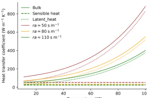
The calculated heat transfer coefficient shows a strong dependence on surface temperature and aerodynamic resis-tance, as shown in Fig. 2. This implies that transient numer-ical models of hydrothermal systems cannot use a fixed heat transfer coefficient at the land surface, because changes in land surface and spring temperature over time change the heat transfer coefficient.
2.3 Boiling temperature
Figure 2.Calculated heat transfer coefficient of the air overlying the land surface and its dependence on the temperature of the land sur-face and aerodynamic resistance (ra). The heat transfer coefficient
is an artificially high value of thermal conductivity that takes into account the contribution of latent and sensible heat flux to surface heat flux.
(2018):
Tmax=3.866 log(P )3+25.151 log(P )2
+103.28 log(P )+179.99, (10)
whereTmaxis the maximum (boiling) temperature in the
sys-tem (◦C) and P is fluid pressure (Pa), which is assumed to be hydrostatic. Using the boiling temperature as an up-per limit ensures that subsurface temup-peratures remain realis-tic in a system where vapour is present. Note however that this approach is a simplification in which the latent heat of vaporization is ignored and in which bulk thermal conduc-tivities are not adjusted for the presence of a vapour phase. Therefore, this is intended as a 1st-order approximation of temperatures in multi-phase flow systems, but for more real-istic models it would be preferable to use multi-phase flow codes such as Hydrotherm (Hayba and Ingebritsen, 1994). Note that the choice for capping modelled temperature by the boiling temperature avoids the high computational ex-pense of including phase transformations in the model code, which would necessitate solving an additional equation for each node and each time step, and which would likely place more constraints on spatial discretization and time step size. 2.4 Erosion and sedimentation
For modelling systems that are active over longer timescales, Beo can take into account erosion or sedimentation by low-ering or raising the land surface over time. This is done in a stepwise fashion, with the default value set to steps of 1 m. The implementation of erosion is important for low-temperature thermochronometers, because it exposes rocks that have been buried deeper and may have experienced
more hydrothermal heating than rocks at the surface that are buffered by surface temperatures.
2.5 Apatite(U–Th)/He thermochronology
The modelled temperature history was used to calculate the response in low-temperature thermochronometer apatite(U– Th)/He (AHe). The AHe thermochronometer is based on the sensitivity of the diffusion of helium in apatite minerals to temperature. At high temperatures helium diffuses out at a rate equal to or higher than the production by radioactive de-cay, whereas at low temperatures helium is retained in the apatite minerals. The AHe thermochronometer is sensitive to temperatures ranging from approximately 40 to 70◦C (Rein-ers et al., 2005). AHe ages were calculated by solving the he-lium production and diffusion equation for apatites using the eigenmode method, following Meesters and Dunai (2002a, b), which is a computationally efficient method that provides the same results as more computationally demanding finite difference methods (Meesters and Dunai, 2002a, b). Helium production and diffusion is described by
∂C ∂t =D∇
2C+S
pU, (11)
whereCis the concentration of helium (mol m−3),Dis the diffusion coefficient of helium (m2s−1) andUis the helium production rate (mol m−3s−1). The termSpdenotes the
prob-ability that an emitted alpha particle stops at locationx, y, z in the apatite crystal (dimensionless), which is required be-cause the long stopping distance of alpha decay (approxi-mately 21 µm) means that some of the helium that is pro-duced by radioactive decay is not retained inside the crystal. The helium age is calculated using the modelled average con-centration of helium in the crystal (Cavg) following
AHe age=Cavg
U . (12)
The helium diffusion model assumes a spherical shape of the apatite crystal and can be compared to measured AHe ages when using an equivalent spherical shape with the same surface-to-volume ratio as the actual crystal (Meesters and Dunai, 2002a).
et al. (1998) instead that do not take radiation damage into account.
The parameter Sp is used to correct He concentration in
the apatite crystal for the chance that alpha particles that are ejected from locations close to the crystal rim end up out-side the crystal. See Meesters and Dunai (2002b) for more details on the implementation of this parameter in the helium diffusion model. I used an alpha stopping distance of 21 µm (Ketcham et al., 2011).
3 Model verification
I first validated the transient conductive heat flow in the nu-merical model using an analytical solution for the cooling of an intrusive in the subsurface. The solution for temperature change of an initially perturbed temperature field is (Carslaw and Jaeger, 1959)
T (z, t )=Tb+Ti−Tb
2
erf
L−x 2√κt
+erf
L+x 2√κt
, (13) whereTbis the background temperature (◦C),Tiis the
tem-perature of the intrusive (◦C),Lis the length of the intrusive (m), x is distance from the intrusive (m) andκ is thermal diffusivity (m2s−1)
Following Ehlers (2005) I use this equation to simulate cooling of an intrusive in the subsurface as a test case for the model code. The numerical and analytical solutions for cooling are shown in Fig. 3. The intrusive body has an ini-tial temperature of 700◦C and stretches from 0 to 500 m dis-tance. The background temperature is 50◦C. The solutions match to within 1.0◦C.
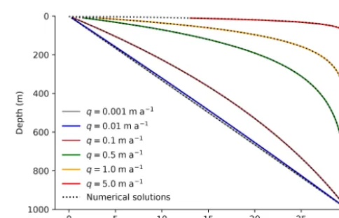
In addition, the performance of the model code was eval-uated using an analytical solution of steady-state heat advec-tion and conducadvec-tion by Bredehoeft and Papaopulos (1965). The solution describes heat advection in a one-dimensional system with fixed temperatures at the top and bottom bound-aries of the model domain. The analytical solution is given by
T =e
((β z)/L)−1
eβ−1 1T +T0 (14)
and
β= −cρqL/K, (15)
whereT is temperature (K),zis depth (m),1T is the tem-perature difference between the top and the bottom of the domain (K), T0is the temperature at the top of the domain
(K), cis heat capacity (J kg−1K−1),ρ is density (kg m−3),
L is length of the domain (m) andK is thermal conductiv-ity (W m−1K−1). A comparison between the numerical solu-tions by Beo and the analytical solusolu-tions shows that the ana-lytical and numerical solutions are identical (Figs. 3 and 4).
Figure 3.Validation of modelled transient conductive heat flow with an analytical solution (Carslaw and Jaeger, 1959) for the cool-ing of an intrusive over time. Solid lines show calculated tempera-tures using the analytical solution at three different time steps. Bro-ken lines show the numerical solution by Beo.
Figure 4. Validation of modelled advective heat flow in a one-dimensional system with an analytical solution (Bredehoeft and Pa-paopulos, 1965). Solid lines show calculated temperatures using the analytical solution and broken lines the numerical solution by Beo.
4 Model usage 4.1 Model input
ElcoLuijendijk/beo/tree/master/manual, last access: 2 Au-gust 2019). The input file can be specified as a command line argument. For instance the command python beo.py example_input_files/Baden.py will run the model using the input file Baden.py in subdirectory
example_input_files. 4.2 Running multiple models
Beo can be used for automated model runs for model sensi-tivity analysis or exploration of parameter space. The class ParameterRanges can contain series of parameter values for any parameter from the main parameter set (i.e. contained in the class ModelParams). The user can choose an option to perform model sensitivity analysis, in which each time a sin-gle parameter is changed while all other parameters are kept at their base value. Alternatively one can choose to generate model runs for each parameter combination, which can be used to explore parameter space.
4.3 Model output and visualization
Beo generates output to comma-separated files, model-specific output files using the Python pickle module, and out-put of the modelled temperatures and fluid fluxes in VTK format. The comma-separated files contain a copy of all in-put parameters for each model run, along with several statis-tics for the model output such as modelled average change in temperatures compared to initial temperatures, modelled temperatures at the surface or user-specified depth slices, modelled AHe data, and comparison to observed values. Modelled temperatures and fluxes can be saved as VTK files that can be used for model visualization using external soft-ware such as Paraview and Visit. In addition, the model re-sults can be saved in a Beo-specific file format that contains all modelled temperature and AHe data. These output files can be used by a separate script (make_figure.py) to au-tomatically generate figures such as the model results shown in this study (Fig. 5).
5 Application
The following section presents models of two active hy-drothermal systems. The first case study consists of a model of the thermal history of the Baden and Schinznach spring system, a hydrothermal system and series of hot springs at the boundary of the Jura Mountains and the Molasse Basin in Switzerland. This study demonstrates the potential and limitations of the use of spring temperatures and discharge to quantify the depth of fluid conduits and the use of low-temperature thermochronology to reconstruct the history of hydrothermal activity. The second case study is a model of borehole temperatures and borehole apatite (U–Th)/He data in a hydrothermal system at the Brigerbad spring in the Rhône Valley in the western Alps, which is based on data
published by Valla et al. (2016). Note that the aim is not to provide detailed case studies but to illustrate the possibilities of the model code. In addition to these examples, a sepa-rate study that uses the model code to quantify the history of the Beowawe hydrothermal system in the Basin and Range Province was published recently (Louis et al., 2019). 5.1 Baden and Schinznach hydrothermal system 5.1.1 Model setup
The model of the Baden and Schinznach spring system is based on a model study by Griesser and Rybach (1989). The total heat flux in the Baden and Schinznach spring system that is used as a case study is 2.4×10⁶W, which was calcu-lated using spring discharge and temperature data reported by Sonney and Vuataz (2008) and an assumed recharge temper-ature of 10◦C. With a background heat flow of 0.07 W m2the
minimum contributing area for the heat output of the springs is 3.5×10⁷m2. This is slightly above the median value for springs in North America reported by Ferguson and Grasby (2011). The model study presented here therefore represents a terrestrial hydrothermal system with a relatively high but not unusual heat output.
The area hosts a number of springs with a temperature of 30 to 47◦C (Sonney and Vuataz, 2008) and an average dis-charge along the fault of 2×10⁻⁵m2s−1. Fluid flow is hosted in a relatively shallow thrust fault that dips around 50◦to a detachment level around 1000 m below the surface, which may be connected to a deeper normal fault (Griesser and Ry-bach, 1989; Malz et al., 2015).
The numerical model is based on a conceptual model shown in Fig. 1. The model only includes the discharge part of the hydrothermal system. Groundwater recharge is much more diffuse than discharge and has a negligible effect on subsurface temperatures in comparison to focused ground-water discharge, as shown for instance by model experiments by Ferguson et al. (2009).
A specified heat flow of 0.07 W m−2 was chosen at the lower boundary (Griesser and Rybach, 1989). For the upper model boundary the air temperature is fixed at 10◦C at an elevation of 2 m above the land surface, and the heat trans-fer at the land transtrans-fer is governed by sensible and latent heat flux following Eqs. (3) to (9). Thermal conductivity was fixed at 2.5 W m−1K−1for the rock matrix, 0.58 W m−1K−1 for the pore fluids and the porosity was assumed to be 0.15. The model experiments run for a total of 15 000 years. This represents the approximate duration of an interglacial stage. The springs may have been inactive during glacial stages of the Pleistocene. During the last glaciation the Jura Mountains and part of the Molasse Basin were covered by an ice sheet (Preusser et al., 2011), which may have blocked groundwater recharge and spring flow.
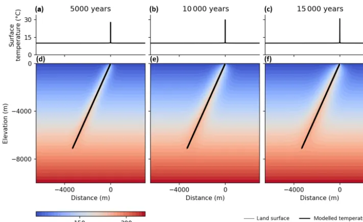
and 10 m in the air layer above the land surface. In total this resulted in 166 285 nodes. The models used a time step size (1t) of 50 years. Experiments with smaller time steps of 0.1 year showed no difference in modelled temperatures. 5.1.2 Sensitivity of modelled spring temperatures A series of model experiments was performed to quantify the effects on the depth, angle and width of fluid conduits on spring temperatures. The base case model assumed a fluid conduit depth of 7 km, a conduit angle of 65◦and a width of 10 m. The modelled subsurface and spring temperatures are shown in Fig. 5. The upward fluid flow raises temperatures in a narrow zone around the fluid conduit. After 15 000 years the area around the fault zone where temperatures are at least 20◦C higher than the background values is approximately 2000 m wide.
The model results show a strong dependence of modelled spring temperatures on the assumed depth of the fluid con-duit (Fig. 6a). The observed temperatures of the Baden and Schinznach spring system are only reached using fluid con-duits that are at least 7 km deep. In addition, comparison of a the effects of fluid conduits dipping 50 and 65◦ shows a strong difference in spring temperatures (Fig. 6a). For a fluid conduit with a low dip angle, the flow path from a particular depth is longer and therefore the amount of heat loss along the way is higher. Modelled spring temperatures for a fluid conduit of 50◦are too low to explain the observed tempera-tures in the system. The model results confirm the hypothesis proposed by Griesser and Rybach (1989) that the fluid source in the Baden and Schinznach hydrothermal system is likely a deep and steeply dipping normal fault that is connected to the more shallow thrust fault that hosts the springs near the surface.
In addition to the depth of the fluid conduit, spring tem-peratures are sensitive to the assumed width of the fault zone (Fig. 6b). The wider the fault zone, the lower the spring tem-perature. Note that in these model runs, the overall flux was kept at 2×10⁻⁵m2s−1, which was redistributed evenly over the width of the fluid conduit. The narrower the fluid conduit, the higher the flow velocity, and the lower the conductive heat loss along the way.
The model experiments also show a strong dependence of spring temperatures on the modelled heat flux at the land surface. The key parameter governing latent and sensible heat flux at the land surface is the aerodynamic resistance (Fig. 2). The value of aerodynamic resistance strongly af-fects spring temperatures. Lower values of resistance, which correspond to more vegetated conditions (Liu et al., 2007), result in higher values of effective thermal conductivity and heat flux at the surface (Fig. 2) and, as a result, lead to lower spring temperatures (Fig. 6b).
5.1.3 Hydrothermal activity and low-temperature thermochronology
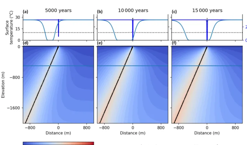
The effect of hydrothermal activity on low-temperature ther-mochronology was explored by using modelled thermal his-tory of the Baden and Schinznach hydrothermal system to calculate AHe ages. For models on longer timescales ex-humation plays a role. Due to the buffering effect of air tem-perature, rocks at deeper levels heat up much more than rocks close to the land surface (Fig. 5). The rate of exhumation therefore determines the strength of the hydrothermal per-turbation of thermochronometer ages. The effect of exhuma-tion rates is explored using two different exhumaexhuma-tion rates, representing slowly exhuming areas such as passive margins (1×10⁻⁴m a−1) and moderate exhumation rates
represent-ing orogens (1×10⁻³m a−1) (Herman et al., 2013). Exhuma-tion rates in the northern part of the Molasse Basin where the springs are located are still under debate, but they equal ap-proximately 1.5 km over the last 5 million years (Cederbom et al., 2011) or 12 million years (von Hagke et al., 2015) (1– 3×10⁴m a−1). Note that to better compare the model results, the initial AHe age, i.e. the AHe age before the start of hy-drothermal activity, was set to the same value for both model experiments.
The results demonstrate that the effect of hydrothermal ac-tivity on thermochronometers is dependent on background exhumation rates. For a model run with a high exhumation rate of 1×10⁻³m a−1the width of the zone at the surface where samples are partially reset is 35 m after 15 000 years, which is 10 m wider than the width of the fluid conduit (25 m) in this model experiment. This means that low-temperature thermochronometers can be used to quantify the history of active hydrothermal systems and hot springs, but only if sam-pling is very dense.
For samples located at 500 m depth thermochronome-ters are affected up to 850 m distance from the fluid conduit (Fig. 8). This means that even over a relatively short timescale of one interglacial stage (∼15 000 years), hydrothermal activity can affect low-temperature ther-mochronometers at the subsurface in large areas. The effect of hydrothermal activity may be important for the interpreta-tion of thermochronometers from boreholes near hydrother-mal systems or areas close to exhumed hydrotherhydrother-mal sys-tems.
5.2 Brigerbad 5.2.1 Model setup
Figure 5.Base case model run for the Baden–Schinznach system, showing modelled subsurface(d–f)and spring(a–c)temperatures at three time slices.
Figure 6.Modelled spring temperatures over time and sensitivity of spring temperatures to the geometry of the fluid conduit and the heat flux at the land surface. The observed present-day temperatures in the springs range from 30 to 47◦C (Sonney and Vuataz, 2008). The base case model uses a fluid conduit depth of 7 km, a width of 10 m, an angle of 65◦, and a value of aerodynamic resistance (ra), which governs
the heat flux at the land surface, of 80 s m−1.
that is located in the valley floor and that forms the contact between the crystalline rocks of the Aar massif and low per-meable sedimentary units of the Helvetic nappe (Buser et al., 2013; Valla et al., 2016). Subsurface temperatures in a 500 m deep borehole close to the springs show a strongly elevated geothermal gradient of approximately 100◦C km−1 that is caused by the upward flow of warm groundwater.
The hydrothermal system was modelled using a simpli-fied setup that uses a wide fault zone that functions as a flow conduit with a maximum depth of 3.5 km and an up-per boundary at a depth of 100 m, where the fault is over-lain by low-permeable Quaternary sediments (Buser et al.,
Figure 7.Modelled surface and subsurface temperatures and AHe ages for three time slices for a model run with a high exhumation rate (1×10⁻³m a−1) and a low exhumation rate (1×10⁻⁴m a−1). Panels(a),(b)and(c)show the modelled temperature at the land surface and modelled AHe ages for surface samples. Panels(d),(e)and(f)show the modelled temperature field in response to upward advective flux along a fault for the model run with a high exhumation rate.
Figure 8.Modelled surface(a–c)and subsurface temperatures(d–f)and AHe ages at the surface and at 500 m depth for three time slices. The model results show the much larger effect of hydrothermal activity on the AHe ages at depth.
was estimated as 230 m2a−1 following reported discharge values of the springs (Sonney and Vuataz, 2008). Following published conceptual models and hydrochemical data (Buser et al., 2013) an estimated 50 % of the total discharge is deep fluid flow through the fault zone, and 50 % consists of
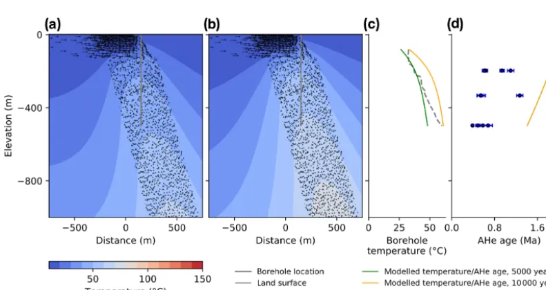
poros-Figure 9.Modelled temperatures and AHe ages for the Brigerbad hydrothermal system after 5000(a)and 10 000(b)years of hydrothermal activity, assuming a narrow flow conduit of a 100 m. The results show a relatively poor fit to the measured borehole temperature data(c).
Figure 10.Modelled temperatures and AHe ages for the Brigerbad hydrothermal system after 5000(a)and 10 000(b)years of hydrothermal activity, assuming a 500 m wide flow conduit. The results show that a wide flow conduit fits the borehole temperature data much better(c), which suggests that a large part of the crystalline bedrock of the Aar massif is permeable enough to channel deep fluids upward. Modelled AHe ages are higher than the observed values(d), which shows that one episode of flow is not sufficient to reduce AHe ages.
ity as 10 %. The total dimensions of the model domain was 5000 m by 5000 m. The mesh contains 116 854 nodes and uses the same cell sizes and time step size as the model exper-iments for the Baden and Schinznach hydrothermal system as described in Sect. 5.1. The duration of modelled hydrother-mal activity was 10 000 years, which roughly corresponds to the time since deglaciation in the western Alps.
Valla et al. (2016) report three AHe samples from a bore-hole near the springs at depths of 167, 333 and 497 m be-low the surface. The samples contained relatively young
of 27◦C km−1, adding the initial background temperature of the samples that is calculated using their present-day depth below the surface and subsequently combining the initial temperature history with the modelled temperature history, which covered the last 10 000 years of the thermal history of the samples.
5.2.2 Results
Initial model experiments that use a narrow flow conduit that corresponds to the typical width of a fault damage zone for a major fault of 100 m (Bense et al., 2013) fail to provide a good fit the borehole temperature record and overpredict temperatures at shallow depths (Fig. 9). The model only pro-vides a good fit when deep groundwater is channelled upward along a relatively wide flow conduit, with a size of 500 m providing a good fit to the temperature data (Fig. 10). This confirms models put forward in earlier studies (Buser et al., 2013) that suggest broad distribution of permeable fractures and fluid flow, as opposed to flow that is confined to a nar-row fault damage zone. The modelled temperatures do still show a misfit, which suggests that the flow paths may be even more distributed and complex than the simplified model shown here.
The thermal history results in modelled AHe ages that are largely unaffected by hydrothermal activity and that range from 1.4 to 2.1 Ma (Fig. 10d). This is much higher than the measured values in the three samples reported by Valla et al. (2016). The modelled hydrothermal heating during 10 000 years is too short to affect AHe ages. The mismatch indicates that hydrothermal activity was active for much longer than the 10 000 years that were modelled here. The system is likely to have been active periodically, during in-terglacial stages.
6 Conclusions
Beo v1.0 is a new open-source code for simulating heat flow and apatite(U–Th)/He thermochronology around hydrother-mal systems. The model code includes a representation of latent and sensible heat flux at the land surface that pro-vides more realistic spring and land surface temperatures than model codes that use a fixed heat flux, temperature or heat transfer coefficient at the land surface. The code pro-vides new opportunities to quantify the geometry of faults and fluid conduits that are required to match observed dis-charge rates and temperatures in systems that host thermal springs. The code can also quantify the thermal footprint of hydrothermal systems at the surface and at depth and pro-vides a tool to quantify the effects of hydrothermal activity on low-temperature thermochronometers. The effects of hy-drothermal activity on thermochronometers depends strongly on the duration of activity, and the code provides new
oppor-tunities to use thermochronometers to quantify the history of hydrothermal systems and hot springs.
Code availability. The source code of Beo version 1.0 was published at Zenodo (Luijendijk, 2018) and is accessible on-line (https://doi.org/10.5281/zenodo.2527844). The source code is also available on a GitHub repository (https://github.com/ ElcoLuijendijk/beo, last access: 2 August 2019; Luijendijk, 2019). The code is distributed under the GNU General Public License, ver-sion 3. The repository contains a readme file with a brief descrip-tion of model installadescrip-tion, usage and output, and a more extensive manual that includes a detailed description of all variables in the in-put data files. In addition, the repository contains several Jupyter notebooks that can be used to reproduce the model benchmarks discussed in Sect. 3 and the input files for the model examples in Sect. 5. Beo v1.0 depends on the generic finite element code Es-cript (Gross et al., 2007a, b, 2008) and the Python modules numpy, scipy and pandas.
Competing interests. The author declares that there is no conflict of interest.
Acknowledgements. The author would like to acknowledge fi-nancial support from startup funding for postdocs grant number 3917542 from the University of Göttingen, DFG German Research Foundation grant LU1947/1 and DFG grant LU1947/3, which is part of the priority programme MB-4D. Thanks are also due to Sarah Louis for drafting Fig. 1 and Sarah Louis, Saskia Köhler and Theis Winter for testing the model code.
Financial support. This research has been supported by the Deutsche Forschungsgemeinschaft (grant nos. LU1947/1 and LU1947/3) and the University of Göttingen (grant no. 3917542).
This open-access publication was funded by the University of Göttingen.
Review statement. This paper was edited by Thomas Poulet and re-viewed by Manolis Veveakis and Peter van der Beek.
References
Achtziger-Zupanˇciˇc, P., Loew, S., and Mariéthoz, G.: A new global database to improve predictions of permeability distribution in crystalline rocks at site scale, J. Geophys. Res.-Sol. Ea., 122, 3513–3539, https://doi.org/10.1002/2017JB014106, 2017. Alduchov, O. A. and Eskridge, R. E.: Improved Magnus form
ap-proximation of saturation vapor pressure, J. Appl. Meteorol., 35, 601–609, 1996.
transport and limited mantle flux in two extensional geothermal systems in the Great Basin, United States, Geology, 39, 195–198, https://doi.org/10.1130/G31557.1, 2011.
Bateni, S. M. and Entekhabi, D.: Relative efficiency of land surface energy balance components, Water Resourc. Res., 48, W04510, https://doi.org/10.1029/2011WR011357, 2012.
Bense, V., Gleeson, T., Loveless, S., Bour, O., and Scibek, J.: Fault zone hydrogeology, Earth-Sci. Rev., 127, 171–192, https://doi.org/10.1016/j.earscirev.2013.09.008, 2013.
Braun, J., van der Beek, P., Valla, P., Robert, X., Herman, F., Glotzbach, C., Pedersen, V., Perry, C., Simon-Labric, T., and Prigent, C.: Quantifying rates of landscape evolution and tec-tonic processes by thermochronology and numerical modeling of crustal heat transport using PECUBE, Tectonophysics, 524–525, 1–28, https://doi.org/10.1016/j.tecto.2011.12.035, 2012. Bredehoeft, J. D. and Papaopulos, I. S.: Rates of
verti-cal groundwater movement estimated from the Earth’s thermal profile, Water Resour. Res., 1, 325–328, https://doi.org/10.1029/WR001i002p00325, 1965.
Buser, M., Eichenberger, U., Jacquod, J., Paris, U., and Vuataz, F.: Geothermie Brig-Glis, Geothermiebohrungen Brigerbad Phase 2: Schlussbericht Phase 2, Tech. rep., Geothermie Brigerbad AG, Brig-Glis, 2013.
Carslaw, H. S. and Jaeger, J. C.: Conduction of heat in solids, Ox-ford University Press, New York, 1959.
Cederbom, C. E., van der Beek, P., Schlunegger, F., Sinclair, H. D., and Oncken, O.: Rapid extensive erosion of the North Alpine foreland basin at 5–4 Ma, Basin Res., 23, 528–550, https://doi.org/10.1111/j.1365-2117.2011.00501.x, 2011. Dempster, T. J. and Persano, C.: Low-temperature
thermochronol-ogy: Resolving geotherm shapes or denudation histories?, Geol-ogy, 34, 73–76, 2006.
Ehlers, T. A.: Computational Tools for Low-Temperature Ther-mochronometer Interpretation, Rev. Mineral. Geochem., 58, 589–622, https://doi.org/10.2138/rmg.2005.58.22, 2005. Farley, K. A.: Helium diffusion from apatite: General behavior as
illustrated by Durango fluorapatite, J. Geophys. Res., 105, 2903– 2914, https://doi.org/10.1029/1999JB900348, 2000.
Ferguson, G. and Grasby, S. E.: Thermal springs and heat flow in North America, Geofluids, 11, 294–301, https://doi.org/10.1111/j.1468-8123.2011.00339.x, 2011. Ferguson, G., Grasby, S. E., and Hindle, S. R.: What do
aque-ous geothermometers really tell us?, Geofluids, 9, 39–48, https://doi.org/10.1111/j.1468-8123.2008.00237.x, 2009. Flowers, R. M., Ketcham, R. A., Shuster, D. L., and Farley, K. A.:
Apatite(U-Th)/He thermochronometry using a radiation dam-age accumulation and annealing model, Geochim. Cosmochim. Ac., 73, 2347–2365, https://doi.org/10.1016/j.gca.2009.01.015, 2009.
Gallagher, K.: Transdimensional inverse thermal history modeling for quantitative thermochronology, J. Geophys. Res.-Sol. Ea., 117, B02408, https://doi.org/10.1029/2011JB008825, 2012. Gautheron, C., Tassan-Got, L., Barbarand, J., and Pagel, M.: Effect
of alpha-damage annealing on apatite (U-Th)/He thermochronol-ogy, Chem. Geol., 266, 157–170, 2009.
Geuzaine, C. and Remacle, J.-F.: Gmsh: A 3-D finite ele-ment mesh generator with built-in pre-and post-processing facilities, Int. J. Numer. Meth. Eng., 79, 1309–1331, https://doi.org/10.1002/nme.2579, 2009.
Gorynski, K. E., Walker, J. D., Stockli, D. F., and Sabin, A.: Ap-atite (U-Th)/He thermochronometry as an innovative geother-mal exploration tool: A case study from the southern Was-suk Range, Nevada, J. Volcanol. Geoth. Res., 270, 99–114, https://doi.org/10.1016/j.jvolgeores.2013.11.018, 2014. Griesser, J.-C. and Rybach, L.: Numerical thermohydraulic
model-ing of deep groundwater circulation in crystalline basement: an example of calibration, in: Hydrogeological Regimes and Their Subsurface Thermal Effects, edited by: Alan E. Beck, Garven, G., and Stegena, L., American Geophysical Union, Washington, D.C., 65–74, https://doi.org/10.1029/GM047p0065, 1989. Gross, L., Bourgouin, L., Hale, A. J., and Muhlhaus,
H.-B.: Interface Modeling in Incompressible Media using Level Sets in Escript, Phys. Earth Planet. In., 163, 23–34, https://doi.org/10.1016/j.pepi.2007.04.004, 2007a.
Gross, L., Cumming, B., Steube, K., and Weatherley, D.: A Python Module for PDE-Based Numerical Modelling, in: Applied Par-allel Computing. State of the Art in Scientific Computing SE – 33, edited by: Kågström, B., Elmroth, E., Dongarra, J., and Wa´sniewski, J., Lecture Notes in Computer Science, Springer Berlin Heidelberg, 4699, 270–279, https://doi.org/10.1007/978-3-540-75755-9_33, 2007b.
Gross, L., Mühlhaus, H., Thorne, E., and Steube, K.: A New Design of Scientific Software Using Python and XML, Pure Appl. Geo-phys., 165, 653–670, https://doi.org/10.1007/s00024-008-0327-7, 2008.
Hayba, D. O. and Ingebritsen, S. E.: The computer model HY-DROTHERM, a three-dimensional finite-difference model to simulate ground-water flow and heat transport in the temperature range of 0 to 1,200 degrees C, Tech. rep., US Geological Survey, Reston, Virginia, https://doi.org/10.3133/wri944045, 1994. Herman, F., Seward, D., Valla, P. G., Carter, A., Kohn, B.,
Wil-lett, S. D., and Ehlers, T. A.: Worldwide acceleration of moun-tain erosion under a cooling climate, Nature, 504, 423–426, https://doi.org/10.1038/nature12877, 2013.
Hickey, K. A., Barker, S. L. L., Dipple, G. M., Arehart, G. B., and Donelick, R. A.: The brevity of hydrothermal fluid flow revealed by thermal halos around giant gold deposits: implica-tions for Carlin-type gold systems, Econ. Geol., 109, 1461–1487, https://doi.org/10.2113/econgeo.109.5.1461, 2014.
Howald, T., Person, M., Campbell, A., Lueth, V., Hofstra, A., Sweetkind, D., Gable, C. W., Banerjee, A., Luijendijk, E., Crossey, L., Karlstrom, K., Kelley, S., and Phillips, F. M.: Ev-idence for long timescale (>1000 years) changes in hydrother-mal activity induced by seismic events, Geofluids, 15, 252–268, https://doi.org/10.1111/gfl.12113, 2015.
Ketcham, R. A., Carter, A., Donelick, R. A., Barbarand, J., and Hurford, A. J.: Improved modeling of fission-track annealing in apatite, Am. Mineral., 92, 799–810, https://doi.org/10.2138/am.2007.2281, 2007.
Ketcham, R. A., Donelick, R. A., Balestrieri, M. L., and Zattin, M.: Reproducibility of apatite fission-track length data and ther-mal history reconstruction, Earth Planet. Sc. Lett., 284, 504–515, https://doi.org/10.1016/j.epsl.2009.05.015, 2009.
Liu, S., Lu, L., Mao, D., and Jia, L.: Evaluating parame-terizations of aerodynamic resistance to heat transfer using field measurements, Hydrol. Earth Syst. Sci., 11, 769–783, https://doi.org/10.5194/hess-11-769-2007, 2007.
Louis, S., Luijendijk, E., Dunkl, I., and Person, M.: Episodic fluid flow in an active fault, Geology, 47, https://doi.org/10.1130/G46254.1, in press, 2019.
Luijendijk, E.: The role of fluid flow in the thermal history of sedimentary basins: Inferences from thermochronology and nu-merical modeling in the Roer Valley Graben, southern Nether-lands, Phd thesis, Vrije Universiteit Amsterdam, available at: http://hdl.handle.net/1871/35433 (last access: 2 August 2019), 2012.
Luijendijk, E.: Beo: model heat flow and thermochronology in hydrothermal systems, https://doi.org/10.5281/zenodo.2527845, 2018.
Malz, A., Madritsch, H., and Kley, J.: Improving 2D seismic in-terpretation in challenging settings by integration of restoration techniques: A case study from the Jura fold-and-thrust belt, Inter-pretation, 3, SAA37–SAA58, https://doi.org/10.1190/INT-2015-0012.1, 2015.
Márton, I., Moritz, R., and Spikings, R.: Application of low-temperature thermochronology to hydrothermal ore deposits: Formation, preservation and exhumation of epithermal gold sys-tems from the Eastern Rhodopes, Bulgaria, Tectonophysics, 483, 240–254, https://doi.org/10.1016/j.tecto.2009.10.020, 2010. McInnes, B. I. A., Evans, N. J., Fu, F. Q., and Garwin, S.:
Applica-tion of Thermochronology to Hydrothermal Ore Deposits, Rev. Mineral. Geochem., 58, 467–498, 2005.
Meesters, A. G. C. A. and Dunai, T. J.: Solving the production-diffusion equation for finite diffusion domains of various shapes Part I. Implications for low-temperature (U-Th)/He thermochronology, Chem. Geol., 186, 333–344, https://doi.org/10.1016/S0009-2541(01)00422-3, 2002a. Meesters, A. G. C. A. and Dunai, T. J.: Solving the
production-diffusion equation for finite production-diffusion domains of various shapes Part II. Application to cases with a-ejection and nonhomoge-neous distribution of the source, Chem. Geol., 186, 57–73, https://doi.org/10.1016/S0009-2541(02)00073-6, 2002b. Monteith, J. L.: Evaporation and surface
tem-perature, Q. J. Roy. Meteor. Soc., 107, 1–27, https://doi.org/10.1002/qj.49710745102, 1981.
National Institute of Standards and Technology: Thermophysical Properties of Fluid Systems, available at: https://webbook.nist. gov/chemistry/fluid/, last access: 13 July 2018.
Person, M. A., Banerjee, A., Hofstra, A., Sweetkind, D., and Gao, Y.: Hydrologic models of modern and fossil geothermal systems in the Great Basin: Genetic implications for epithermal Au-Ag and Carlin-type gold deposits, Geosphere, 4, 888–917, 2008.
Preusser, F., Graf, H. R., Keller, O., Krayss, E., and Schlüchter, C.: Quaternary glaciation history of northern Switzerland, Quater-nary Sci. J., 60, 282–305, https://doi.org/10.3285/eg.60.2-3.06, 2011.
Ranjram, M., Gleeson, T., and Luijendijk, E.: Is the perme-ability of crystalline rock in the shallow crust related to depth, lithology, or tectonic setting?, Geofluids, 15, 106–119, https://doi.org/10.1111/gfl.12098, 2015.
Reiners, P. W., Ehlers, T. A., and Zeitler, P. K.: Past, present, and future of thermochronology, Rev. Mineral. Geochem., 58, 1–18, https://doi.org/10.2138/rmg.2005.58.1, 2005.
Saad, Y. and Schultz, M.: GMRES: A Generalized Minimal Resid-ual Algorithm for Solving Nonsymmetric Linear Systems, SIAM J. Sci. Stat. Comp., 7, 856–869, https://doi.org/10.1137/0907058, 1986.
Shuster, D. L., Flowers, R. M., and Farley, K. A.: The in-fluence of natural radiation damage on helium diffusion ki-netics in apatite, Earth Planet. Sc. Lett., 249, 148–161, https://doi.org/10.1016/j.epsl.2006.07.028, 2006.
Sonney, R. and Vuataz, F. D.: Properties of geothermal fluids in Switzerland: A new interactive database, Geothermics, 37, 496– 509, https://doi.org/10.1016/j.geothermics.2008.07.001, 2008. Valla, P. G., Rahn, M., Shuster, D. L., and van der Beek,
P. A.: Multi-phase late-Neogene exhumation history of the Aar massif, Swiss central Alps, Terra Nova, 28, 383–393, https://doi.org/10.1111/ter.12231, 2016.
Volpi, G., Magri, F., Frattini, P., Crosta, G. B., and Riva, F.: Groundwater-driven temperature changes at thermal springs in response to recent glaciation: Bormio hydrothermal sys-tem, Central Italian Alps, Hydrogeol. J., 25, 1967–1984, https://doi.org/10.1007/s10040-017-1600-6, 2017.
von Hagke, C., Luijendijk, E., Ondrak, R., and Lindow, J.: Quanti-fying erosion rates in the Molasse basin using a high resolution data set and a new thermal model, Geotectonic Research, 97, 94– 97, https://doi.org/10.1127/1864-5658/2015-36, 2015.
Whipp, D. M. and Ehlers, T. A.: Influence of groundwater flow on thermochronometer-derived exhumation rates in the central Nepalese Himalaya, Geology, 35, 851–854, 2007.
Wieck, J., Person, M. A., and Strayer, L.: A finite element method for simulating fault block motion and hydrothermal fluid flow within rifting basins, Water Resour. Res., 31, 3241–3258, 1995. Wolf, R. A., Farley, K. A., and Kass, D. M.: Modeling of the