Further Evaluation of Squeezing Flow and Heat Transfer of non-Newtonian Fluid with Nanoparticles Conveyed through Vertical Parallel Plates

AUT Journal of Mechanical Engineering

AUT J. Mech. Eng., 3(1) (2019) 15-24 DOI: 10.22060/ajme.2018.14586.5733

Further Evaluation of Squeezing Flow and Heat Transfer of non-Newtonian Fluid

with Nanoparticles Conveyed through Vertical Parallel Plates

A. T. Akinshilo1*_{, A. Adingwupu}2_{, J. Olofinkua}1

1 _{Department of Mechanical Engineering, Faculty of Engineering, University of Lagos, Lagos, Nigeria}

2 _{Department of Mechanical Engineering, College of Engineering, Igbinedion University Okada, Benin, Nigeria}

ABSTRACT: In this paper, the study of squeezing flow of sodium alginate (SA) a non-Newtonian fluid whose rate of shear is not constant with viscosity flows through a medium transporting nanoparticles of silver (Ag) and Alumina (Al₂O₃). The flow medium is a flat parallel plate arranged vertically against each other under steady flow condition. As the flow process arising from the mechanics can be described by ordinary nonlinear differential equation, the Adomian decomposition method been an effective, yet simple method is adopted to analyze the non-linear differential equation. This is used to investigate effect of squeezing flow and heat transfer on the nanofluid. Analytical results reported graphically depicts the effect of squeezing flow on heat transfer utilizing silver nanoparticles shows decreasing temperature distribution for plates coming together while as plates moves apart temperature distribution decreases further. Similar trend is observed adopting the alumina nanoparticle. However the silver nanoparticle having better thermal properties compared with alumina demonstrates higher heat transfer rate due to effect of varying fluid kinematic viscosity on heat exchange. Results generated from the study when compared with existing literature are in good agreement. Therefore study proves a good emphasis for the improvement of sodium alginate transport in biomedical, pharmaceuticals, manufacturing and chemical processes amongst others.

Review History:

Received: 10 June 2018 Revised: 7 October 2018 Accepted: 20 November 2018 Available Online: 1 December 2018

Keywords:

Parallel plates Sodium alginate Nanoparticles

Adomian decomposition method Squeezing flow

15 1- Introduction

The increasing relevance of the sodium alginate, a non-Newtonian fluid in modern day science is due to its wide practical use. Applications including biomedical, pharmaceuticals and manufacturing. Vast effort has been devoted by scientist and engineers to this study owing to influence of rate of shearing on fluid viscosity. The physical phenomena of the sodium alginate in engineering process such as paper production, tissue formation engineering, textile and pharmaceuticals are described by constitutive relations which are nonlinear and of higher order.

In earlier effort to illustrate flow process, Ganji and Kachapi [1] analyzed nonlinear equations in fluids, using numerical and analytical schemes for providing solutions to differential equations while Ziabakhsh and Domairry [2] investigated the effects of natural convection on the flow of a non-Newtonian fluid between two vertical parallel plates. Also the heat and mass transfer effect of unsteady squeezing flow was presented by Mustafa et al. [3] between two parallel plates. Siddiqui et al. [4] presented the unsteady viscous squeezing fluid flow between parallel plates in the presence of magnetic force field .The thermodynamic analysis of third grade fluid was studied by Adesanya and Falade [5] were they presented the rate of entropy generation of the fluid flowing between horizontal parallel plates saturated with porous materials. Hoshyar et al. [6] adopted the homotopy analysis method to study the unsteady incompressible fluid flow between parallel plates. The effect of variable viscosity on fluid flow between parallel plates with shear heating was demonstrated by Myers et al. [7]. Kargar and Akbarzade [8] investigated non-Newtonian

fluid flow between two infinitely long vertical parallel plates using both analytical and numerical approach.

Thermal conductivity of base fluids such as water, glycol and oils have been considerable improved upon the addition of nanometer sized metallic particles. As this enhances it thermal conductivity to about three times its state. Considerably improving the overall transport energy of the base fluid. Making it potentially useful in processes including fuel cells, microelectronic process and medicine. Creative approach such as this has been widely adopted by researchers in the investigation and study of flow and heat transfer properties of fluid [9-22].

A. T. Akinshilo et al., AUT J. Mech. Eng., 3(1) (2019) 15-24, DOI: 10.22060/ajme.2018.14586.5733

16 descritization.

From past literatures, no study as considered a comparative analysis of squeezing flow of the nanofluid with sodium alginate as base fluid. Therefore this current paper aims at investigating and providing a comparative analysis of the squeezing flow effect on the non-Newtonian sodium alginate adopting nanoparticles of silver (Ag) and Alumina (Al₂O₃). The ADM is employed as the suitable method of analysis.

2- Model Development and Analytical Solution

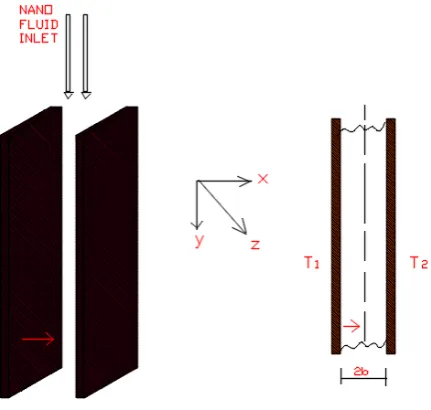
A non-Newtonian sodium alginate flows steadily under natural convection between two plates placed at a distance 2b vertically against each other. The walls are held at constant temperature but opposite in magnitude as illustrated in the problems model, Fig. 1. This is such that temperature difference causes a rise and fall of fluid near the wall. The formulation of the model development of the two component mix is developed following the assumptions that the fluid is incompressible, nanoparticles and fluid are in thermal equilibrium to each other and constant wall temperature. As illustrated from the boundary condition, plates and nanofluid are at equal velocity connoting the no slip condition. While constant temperature but magnitude difference leads to nanofluid rise near the left plate and fall near the right. Following the model proposed by [8,11] introducing the squeezing flow and nanofluid parameters.

The governing equation based on the assumption above can be reduced to ordinary pairs of differential equation. This is presented as:

(

)

(

)

(

)

(

)

2 2 2 3 2 2

2 4 2

3 2

2 3 0

1 2 3

2 2 0 1 2 1 2 2 2. 1 2 0 2 6 2

6 _{, , , ,}

( ) ,Pr , ( ) ( ) 0 0 , 1 , 2 6 f m p

nf nf nf

f f f _{p f}

f p f f

c

p f f f

m

d v dv d v _{T T g}

dx dx dx

dv dv _k d

dx dx dx

C

v A A A

G C

C v

E

C T T k

T T S T T

d V _{S A}

dX

b _V v

V µ β ρ γ θ µ β ρ β ρ µ δ µ ρ µ ρ µ ρ ρ ρ ρ θ δ α υ φ   + _{ } + −     ₊   ₊         = = = = = = − − = − + = − = = =

(

)

(

)

(

)

(

)

2 2 2 5 2 2 2 2 2 2.5 2 2 2 3 4 3 2.5 1

. rS 1

1

2 . .Pr. 0

1

(1 )( ) ( )

(1 )

2 2 ( )

2 ( )

0,

nf f s

p _nf p f p s

f nf

s f f s

nf

f s f f s

d V d V

dX dX

A

d _{Ec P} d V

dX A dX

dV Ec

A dX

C C C

k k k k

k A

k k k k k

v θ θ _φ δ ρ φ ρ φρ ρ φ ρ φ ρ µ µ φ φ φ θ −    +           + _{ } − _{ }      _  + _{  } =     = − + = − + = − + − − = = + − − = 2 2 2.5 1 2 0.5 0, 0.5

(v) 6 (1 )

xx

v

dv d v

L SA dx dx θ δ φ θ = = = −   = − − _{ } +   (1)

(

)

(

)

(

)

(

)

2 2 2 3 2 2

2 4 2

3 2

2 3 0

1 2 3

2 2 0 1 2 1 2 2 2. 1 2 0 2 6 2

6 _{, , , ,}

( ) ,Pr , ( ) ( ) 0 0 , 1 , 2 6 f m p

nf nf nf

f f f _{p f}

f p f f

c

p f f f

m

d v dv d v _{T T g}

dx dx dx

dv dv _k d

dx dx dx

C

v A A A

G C

C v

E

C T T k

T T S T T

d V _{S A}

dX

b _V v

V µ β ρ γ θ µ β ρ β ρ µ δ µ ρ µ ρ µ ρ ρ ρ ρ θ δ α υ φ   + _{ } + −     ₊   ₊         = = = = = = − − = − + = − = = =

(

)

(

)

(

)

(

)

2 2 2 5 2 2 2 2 2 2.5 2 2 2 3 4 3 2.5 1

. rS 1

1

2 . .Pr. 0

1

(1 )( ) ( )

(1 )

2 2 ( )

2 ( )

0,

nf f s

p _nf p f p s

f nf

s f f s

nf

f s f f s

d V d V

dX dX

A

d _{Ec P} d V

dX A dX

dV Ec

A dX

C C C

k k k k

k A

k k k k k

v θ θ _φ δ ρ φ ρ φρ ρ φ ρ φ ρ µ µ φ φ φ θ −    +           + _{ } − _{ }      _  + _{  } =     = − + = − + = − + − − = = + − − = 2 ₂ 2.5 1 2 0.5 0, 0.5

(v) 6 (1 )

xx

v

dv d v

L SA dx dx θ δ φ θ = = = −   = − − _{ } +   (2)

where the dimensionless parameters take the forms:

(

)

(

)

(

)

(

)

2 2 2 3 2 2

2 4 2

3 2

2 3 0

1 2 3

2 2 0 1 2 1 2 2 2. 1 2 0 2 6 2

6 _{, , , ,}

( ) ,Pr , ( ) ( ) 0 0 , 1 , 2 6 f m p

nf nf nf

f f f _{p f}

f p f

f c

p f f f

m

d v dv d v _{T T g}

dx dx dx

dv dv _kd

dx dx dx

C

v A A A

G C

C v

E

C T T k

T T S T T

d V _{S A}

dX

b _V v

V µ β ρ γ θ µ β ρ β ρ µ δ µ ρ µ ρ µ ρ ρ ρ ρ θ δ α υ φ   + _{ } + −     ₊   ₊         = = = = = = − − = − + = − = = =

(

)

(

)

(

)

(

)

2 2 2 5 2 2 2 2 2 2.5 2 2 2 3 4 3 2.5 1

. rS 1

1

2 . .Pr. 0

1

(1 )( ) ( )

(1 )

2 2 ( )

2 ( )

0,

nf f s

p _nf p f p s

f nf

s f f s

nf

f s f f s

d V d V

dX dX

A

d _{Ec P} d V

dX A dX

dV Ec

A dX

C C C

k k k k

k A

k k k k k

v θ θ _φ δ ρ φ ρ φρ ρ φ ρ φ ρ µ µ φ φ φ θ −    +           + _{ } − _{ }      _  + _{  } =     = − + = − + = − + − − = = + − − = 2 2 2.5 1 2 0.5 0, 0.5

(v) 6 (1 )

xx

v

dv d v

L SA dx dx θ δ φ θ = = = −   = − − _{ } +   (3)

With the aid of non-dimensional parameter Eq. (3). The Eqs. (1) and (2) are expressed as:

(

)

(

)

(

)

(

)

2 2 2 3 2 2

2 4 2

3 2

2 3 0

1 2 3

2 2 0 1 2 1 2 2 2. 1 2 0 2 6 2

6 _{, , , ,}

( ) ,Pr , ( ) ( ) 0 0 , 1 , 2 6 f m p

nf nf nf

f f f _{p f}

f p f

f c

p f f f

m

d v dv d v _{T T g}

dx dx dx

dv dv _kd

dx dx dx

C

v A A A

G C

C v

E

C T T k

T T S T T

d V _{S A}

dX

b _V v

V µ β ρ γ θ µ β ρ β ρ µ δ µ ρ µ ρ µ ρ ρ ρ ρ θ δ α υ φ   + _{ } + −     ₊   ₊         = = = = = = − − = − + = − = = =

(

)

(

)

(

)

(

)

2 2 2 5 2 2 2 2 2 2.5 2 2 2 3 4 3 2.5 1

. rS 1

1

2 . .Pr. 0

1

(1 )( ) ( )

(1 )

2 2 ( )

2 ( )

0,

nf f s

p _nf p f p s

f nf

s f f s

nf

f s f f s

d V d V

dX dX

A

d _{Ec P} d V

dX A dX

dV Ec

A dX

C C C

k k k k

k A

k k k k k

v θ θ _φ δ ρ φ ρ φρ ρ φ ρ φ ρ µ µ φ φ φ θ −    +           + _{ } − _{ }      _  + _{  } =     = − + = − + = − + − − = = + − − = 2 2 2.5 1 2 0.5 0, 0.5

(v) 6 (1 )

xx

v

dv d v

L SA dx dx θ δ φ θ = = = −   = − − _{ } +   (4)

(

)

(

)

(

)

(

)

2 2 2 3 2 2

2 4 2

3 2

2 3 0

1 2 3

2 2 0 1 2 1 2 2 2. 1 2 0 2 6 2

6 _{, , , ,}

( ) ,Pr , ( ) ( ) 0 0 , 1 , 2 6 f m p

nf nf nf

f f f _{p f}

f p f

f c

p f f f

m

d v dv d v _{T T g}

dx dx dx

dv dv _kd

dx dx dx

C

v A A A

G C

C v

E

C T T k

T T S T T

d V _{S A}

dX

b _V v

V µ β ρ γ θ µ β ρ β ρ µ δ µ ρ µ ρ µ ρ ρ ρ ρ θ δ α υ φ   + _{ } + −     ₊   ₊         = = = = = = − − = − + = − = = =

(

)

(

)

(

)

(

)

2 2 2 5 2 2 2 2 2 2.5 2 2 2 3 4 3 2.5 1

. rS 1

1

2 . .Pr. 0

1

(1 )( ) ( )

(1 )

2 2 ( )

2 ( )

0,

nf f s

p _nf p f p s

f nf

s f f s

nf

f s f f s

d V d V

dX dX

A

d _{Ec P} d V

dX A dX

dV Ec

A dX

C C C

k k k k

k A

k k k k k

v θ θ _φ δ ρ φ ρ φρ ρ φ ρ φ ρ µ µ φ φ φ θ −    +           + _{ } − _{ }      _  + _{  } =     = − + = − + = − + − − = = + − − = 2 2 2.5 1 2 0.5 0, 0.5

(v) 6 (1 )

xx

v

dv d v

L SA dx dx θ δ φ θ = = = −   = − − _{ } +   (5)

where the effective density ρ_nf, effective dynamic viscosity

μ_nf, heat capacitance(ρC_p)_nf and thermal conductivity k_nf of the nanofluid are defined as follows [40]:

(

)

(

)

(

)

(

)

2 2 2 3 2 2

2 4 2

3 2

2 3 0

1 2 3

2 2 0 1 2 1 2 2 2. 1 2 0 2 6 2

6 _{, , , ,}

( ) ,Pr , ( ) ( ) 0 0 , 1 , 2 6 f m p

nf nf nf

f f f _{p f}

f p f

f c

p f f f

m

d v dv d v _{T T g}

dx dx dx

dv dv _kd

dx dx dx

C

v A A A

G C

C v

E

C T T k

T T S T T

d V _{S A}

dX

b _V v

V µ β ρ γ θ µ β ρ β ρ µ δ µ ρ µ ρ µ ρ ρ ρ ρ θ δ α υ φ   + _{ } + −     ₊   ₊         = = = = = = − − = − + = − = = =

(

)

(

)

(

)

(

)

2 2 2 5 2 2 2 2 2 2.5 2 2 2 3 4 3 2.5 1

. rS 1

1

2 . .Pr. 0

1

(1 )( ) ( )

(1 )

2 2 ( )

2 ( )

0,

nf f s

p _nf p f p s

f nf

s f f s

nf

f s f f s

d V d V

dX dX

A

d _{Ec P} d V

dX A dX

dV Ec

A dX

C C C

k k k k

k A

k k k k k

v θ θ _φ δ ρ φ ρ φρ ρ φ ρ φ ρ µ µ φ φ φ θ −    +           + _{ } − _{ }      _  + _{  } =     = − + = − + = − + − − = = + − − = 2 2 2.5 1 2 0.5 0, 0.5

(v) 6 (1 )

xx

v

dv d v

L SA dx dx θ δ φ θ = = = −   = − − _{ } +   (6)

(

)

(

)

(

)

(

)

2 2 2 3 2 2

2 4 2

3 2

2 3 0

1 2 3

2 2 0 1 2 1 2 2 2. 1 2 0 2 6 2

6 _{, , , ,}

( ) ,Pr , ( ) ( ) 0 0 , 1 , 2 6 f m p

nf nf nf

f f f _{p f}

f p f

f c

p f f f

m

d v dv d v _{T T g}

dx dx dx

dv dv _kd

dx dx dx

C

v A A A

G C

C v

E

C T T k

T T S T T

d V _{S A}

dX

b _V v

V µ β ρ γ θ µ β ρ β ρ µ δ µ ρ µ ρ µ ρ ρ ρ ρ θ δ α υ φ   + _{ } + −     ₊   ₊         = = = = = = − − = − + = − = = =

(

)

(

)

(

)

(

)

2 2 2 5 2 2 2 2 2 2.5 2 2 2 3 4 3 2.5 1

. rS 1

1

2 . .Pr. 0

1

(1 )( ) ( )

(1 )

2 2 ( )

2 ( )

0,

nf f s

p _nf p f p s

f nf

s f f s

nf

f s f f s

d V d V

dX dX

A

d _{Ec P} d V

dX A dX

dV Ec

A dX

C C C

k k k k

k A

k k k k k

v θ θ _φ δ ρ φ ρ φρ ρ φ ρ φ ρ µ µ φ φ φ θ −    +           + _{ } − _{ }      _  + _{  } =     = − + = − + = − + − − = = + − − = 2 2 2.5 1 2 0.5 0, 0.5

(v) 6 (1 )

xx

v

dv d v

L SA dx dx θ δ φ θ = = = −   = − − _{ } +   (7)

(

)

(

)

(

)

(

)

2 2 2 3 2 2

2 4 ₂

3 2

2 3 0

1 2 3

2 2 0 1 2 1 2 2 2. 1 2 0 2 6 2

6 _{, , , ,}

( ) ,Pr , ( ) ( ) 0 0 , 1 , 2 6 f m p

nf nf nf

f f f _{p f}

f p f

f c

p f f f

m

d v dv d v _{T T g}

dx dx dx

dv dv _kd

dx dx dx

C

v A A A

G C

C v

E

C T T k

T T S T T

d V _{S A}

dX

b _V v

V µ β ρ γ θ µ β ρ β ρ µ δ µ ρ µ ρ µ ρ ρ ρ ρ θ δ α υ φ   + _{ } + −     ₊   ₊         = = = = = = − − = − + = − = = =

(

)

(

)

(

)

(

)

2 2 2 5 2 2 2 2 2 2.5 2 2 2 3 4 3 2.5 1

. rS 1

1

2 . .Pr. 0

1

(1 )( ) ( )

(1 )

2 2 ( )

2 ( )

0,

nf f s

p _nf p f p s

f nf

s f f s

nf

f s f f s

d V d V

dX dX

A

d _{Ec P} d V

dX A dX

dV Ec

A dX

C C C

k k k k

k A

k k k k k

v θ θ _φ δ ρ φ ρ φρ ρ φ ρ φ ρ µ µ φ φ φ θ −    +           + _{ } − _{ }      _  + _{  } =     = − + = − + = − + − − = = + − − = 2 ₂ 2.5 1 2 0.5 0, 0.5

(v) 6 (1 )

xx

v

dv d v

L SA dx dx θ δ φ θ = = = −   = − − _{ } +   (8)

(

)

(

)

(

)

(

)

2 2 2 3 2 2

2 4 ₂

3 2

2 3 0

1 2 3

2 2 0 1 2 1 2 2 2. 1 2 0 2 6 2

6 _{, , , ,}

( ) ,Pr , ( ) ( ) 0 0 , 1 , 2 6 f m p

nf nf nf

f f f _{p f}

f p f

f c

p f f f

m

d v dv d v _{T T g}

dx dx dx

dv dv _kd

dx dx dx

C

v A A A

G C

C v

E

C T T k

T T S T T

d V _{S A}

dX

b _V v

V µ β ρ γ θ µ β ρ β ρ µ δ µ ρ µ ρ µ ρ ρ ρ ρ θ δ α υ φ   + _{ } + −     ₊   ₊         = = = = = = − − = − + = − = = =

(

)

(

)

(

)

(

)

2 2 2 5 2 2 2 2 2 2.5 2 2 2 3 4 3 2.5 1

. rS 1

1

2 . .Pr. 0

1

(1 )( ) ( )

(1 )

2 2 ( )

2 ( )

0,

nf f s

p _nf p f p s

f nf

s f f s

nf

f s f f s

d V d V

dX dX

A

d _{Ec P} d V

dX A dX

dV Ec

A dX

C C C

k k k k

k A

k k k k k

v θ θ _φ δ ρ φ ρ φρ ρ φ ρ φ ρ µ µ φ φ φ θ −    +           + _{ } − _{ }      _  + _{  } =     = − + = − + = − + − − = = + − − = 2 ₂ 2.5 1 2 0.5 0, 0.5

(v) 6 (1 )

xx

v

dv d v

L SA dx dx θ δ φ θ = = = −   = − − _{ } +   (9)

Taking the boundary condition as

(

)

(

)

(

)

(

)

2 2 2 3 2 2

2 4 ₂

3 2

2 3 0

1 2 3

2 2 0 1 2 1 2 2 2. 1 2 0 2 6 2

6 _{, , , ,}

( ) ,Pr , ( ) ( ) 0 0 , 1 , 2 6 f m p

nf nf nf

f f f _{p f}

f p f

f c

p f f f

m

d v dv d v _{T T g}

dx dx dx

dv dv _kd

dx dx dx

C

v A A A

G C

C v

E

C T T k

T T S T T

d V _{S A}

dX

b _V v

V µ β ρ γ θ µ β ρ β ρ µ δ µ ρ µ ρ µ ρ ρ ρ ρ θ δ α υ φ   + _{ } + −     ₊   ₊         = = = = = = − − = − + = − = = =

(

)

(

)

(

)

(

)

2 2 2 5 2 2 2 2 2 2.5 2 2 2 3 4 3 2.5 1

. rS 1

1

2 . .Pr. 0

1

(1 )( ) ( )

(1 )

2 2 ( )

2 ( )

0,

nf f s

p _nf p f p s

f nf

s f f s

nf

f s f f s

d V d V

dX dX

A

d _{Ec P} d V

dX A dX

dV Ec

A dX

C C C

k k k k

k A

k k k k k

v θ θ _φ δ ρ φ ρ φρ ρ φ ρ φ ρ µ µ φ φ φ θ −    +           + _{ } − _{ }      _{ } + _{  } =     = − + = − + = − + − − = = + − − = 2 2 2.5 1 2 0.5 0, 0.5

(v) 6 (1 )

xx

v

dv d v

L SA dx dx θ δ φ θ = = = −   = − − _{ } +   (10)

The preferred analytical scheme, which is the ADM. Is adopted for providing approximate solutions to the ordinary differential, nonlinear, second order equations. Upon the application of the ADM to the Eqs. (3) and (4), the governing Fig. 1. Physical model of the problem

Density (kg/m3₎

Specific heat capacity (J/kg.K) Thermal conductivity (W/m.K)

Sodium Alginate (SA) 989 4175 0.637

Silver (Ag) 10500 235 429

Alumina (Al₂O₃) 3970 765 40 Table 1. Thermo physical properties of sodium alginate, silver