https://doi.org/10.5194/gmd-11-5085-2018 © Author(s) 2018. This work is distributed under the Creative Commons Attribution 4.0 License.
OLYMPUS v1.0: development of an integrated air pollutant and
GHG urban emissions model – methodology and calibration
over greater Paris
Arthur Elessa Etuman and Isabelle Coll
Laboratoire Interuniversitaire des Systèmes Atmosphériques (LISA), UMR CNRS 7583, Université Paris Est Créteil et Université Paris Diderot, Institut Pierre Simon Laplace (IPSL), Créteil, France
Correspondence:Arthur Elessa Etuman ([email protected]) Received: 22 June 2018 – Discussion started: 30 July 2018
Revised: 24 October 2018 – Accepted: 10 November 2018 – Published: 12 December 2018
Abstract.Air pollutants and greenhouse gases have many ef-fects on health, the economy, urban climate and atmospheric environment. At the city level, the transport and heating sec-tors contribute significantly to air pollution. In order to quan-tify the impact of urban policies on anthropogenic air pol-lutants, the main processes leading to emissions need to be understood: they principally include mobility for work and leisure as well as household behavior, themselves impacted by a variety of social parameters.
In this context, the OLYMPUS modeling platform has been designed for environmental decision support. It gen-erates a synthetic population of individuals and defines the mobility of each individual in the city through an activity-based approach of travel demand. The model then spatial-izes road traffic by taking into account congestion on the road network. It also includes a module that estimates the energy demand of the territory by calculating the unit energy consumption of households and the commercial–institutional sector. Finally, the emissions associated with all the modeled activities are calculated using the COPERT emission factors for traffic and the European Environmental Agency (EEA) methodology for heating-related combustion. The compari-son of emissions with AIRPARIF’s regional inventory shows discrepancies that are consistent with differences in assump-tions and input data, mainly in the sense of underestima-tion. The methodological choices and the potential ways of improvement, including the refinement of traffic congestion modeling and of the transport of goods, are discussed.
1 Introduction
As the world’s population grows, the share of the popula-tion living in urban areas also increases (United Napopula-tions, 2014). These areas can be described as hubs of activity with a substantial density of individuals, buildings, transport net-works and employment centers. All the human activities as-sociated with these metropolises induce a large local con-sumption of fossil energy and natural resources, favoring the concentration of a great variety of nuisances (noise, stress, pollution). Among the most emitting activities induced by the city, one can find – according to the IPCC nomenclature (IPCC, 1996) – energy consumption, industrial processes, the use of solvents and agriculture. However, at the city level, anthropogenic emissions are mainly the result of the com-bustion of road transportation fuels and residential, commer-cial and institutional heating and boiling, which account for more than half of total urban emissions (International En-ergy Agency, 2016). In Europe in particular, some cities are associated with the massive use of passenger cars (and some-times even diesel fuel), which further increases their poten-tial for the emission of air pollutants. In these areas, road transport and the production of electricity and heat represent more than 60 % of anthropogenic emissions of nitrogen ox-ides (NOx), particles smaller than 2.5 µm (PM2.5) and non-methane volatile organic compounds (NMVOCs) (Interna-tional Energy Agency, 2016). Quantitatively, although sulfur oxide (SOx) emissions have declined since the 1990s, NOx
result, even though exposure to short-lived peaks is decreas-ing, the exposure of the population to chronic pollution is still high in European urban areas (EEA, 2015), and 94 % of ex-ceedances of the short-term limit value for PM10have been observed in urban or suburban areas (EEA, 2016). Air pollu-tion has serious consequences for human health. Recent esti-mates confirm the considerable burden of diseases associated with air pollution in urban areas, which results in pulmonary and cardiovascular diseases, cancer, certain types of diabetes in adults, and attacks on the neuronal development of very young populations (World Health Organization, 2013). From an economic perspective, it leads to high health care costs and to a significant drop in productivity for businesses. At the same time, societal questions related to the degradation of air quality arise. According to a survey carried out between 2007 and 2015 on behalf of the European Commission (European Commission, 2010), there are nine European Union capitals among the 20 cities with the lowest rate of people satisfied with the quality of the urban air, with the greatest decrease in the satisfaction index being observed in greater Paris.
Given the systemic nature of urban areas, it became clear that we could no longer ignore the links between urban morphology, individuals, energy consumption and pollutant emissions when dealing with environmental urban issues (Le Néchet, 2010) – urban morphology (or urban form) is de-fined here as the patterns of space occupation by a metropo-lis measured by the density and degree of hierarchization of the different urban cores. Indeed, the IPCC has recently rec-ognized the impact of four variables linked with urban mor-phology (density, mixed land use, connectivity and accessi-bility) on energy consumption, climate and air quality issues. The effects of these four variables are expressed through the elasticity of the number of kilometers traveled, a parameter called “vehicle km traveled – VKT” (Seto et al., 2014). First, urban density, which reflects the spatial distribution of popu-lation, employment, housing or transport structures, impacts mobility choices through the deployment and sustainabil-ity of the local transport supply. Mixed land use (estimated by local employment-to-household ratios or household-to-services ratios, for example) also determines the morphology of the city, since a reduction in land use diversity reinforces the centrality of activities and shapes the population mobility for all trip purposes. Connectivity corresponds to the spatial structure and density of roads and pedestrian paths: in partic-ular, it has been shown to promote walking. Finally, acces-sibility – defined as access to jobs, housing and services – can help reduce VKT, particularly for professional mobility (commuting). The way in which the urban form, the distri-bution of employment areas and the transport supply impose spatial interactions between individuals can be identified as the urban organization (Bretagnolle et al., 2010). Such an or-ganization appears clearly dependent on the cost of energy. And when the relations between urban form and daily mo-bility are questioned, they invariably lead to classic issues in the literature (Melia et al., 2011; Le Néchet, 2010; Schindler
and Caruso, 2014): spread urban forms would be the most energy-consuming structures, while a strong hierarchy be-tween urban centers with an increase in central compactness would help reduce the distance to jobs and the use of a car. Moreover, dense urban forms, unlike spread urban forms, al-low for a more efficient use of energy through the use of dense networks (heating, electricity, gas). However, it seems that dense urban structures also tend to reduce the share of local trips undertaken by sustainable modes due to increased metropolitan integration.
There are still few research projects in the literature that have included a large number of urban components into emission scenarios dedicated to AQMs (Manins, 1995; Mar-quez and Smith, 1999; Martins, 2012; De Ridder et al., 2008). Prospective modeling research in the 2000s has re-vealed the determining role of mobility and city configura-tion (considered as the spatial organizaconfigura-tion of buildings, ser-vices and networks) in the exposure of individuals, but the study focused on academic situations (Borrego et al., 2006). However, over the last decade, social components have pro-gressively been integrated into urban emissions models, such as TASHA-MATSIM-MOBILE6.2C (Hao et al., 2010) and TRANUS-TREM (Bandeira et al., 2011), which are now able to quantify the impact of urban policies on road traffic emis-sions through carpooling, transportation fleet technology and individual modal choice. The strength of these models is linked to the implementation of a microsimulation approach based on individual choice, which depends on economic pa-rameters. However, most of the applications focused on road traffic emissions only (Hatzopoulou et al., 2008; Hülsmann et al., 2014), whereas in the current context that places partic-ular emphasis on the emerging concept of sustainable cities, it is necessary to take into account all air pollutant emissions related to energy consumption, insofar as they interact with air quality and climate change. In particular, there is a need to also take into account small combustion emissions (both residential and commercial) and their related policies to go further in the realism of the urban scenarios and to address the issue of air quality levers in a more holistic manner.
OLYMPUS is an emission model designed to produce a new generation of emission scenarios for air quality models (AQMs) at the scale of an urban area. It aims to meet the need described above to produce emission scenarios that in-tegrate the interactions between the geographical aspects of the city, its population, the organization of buildings and ur-ban networks, in order to produce a more comprehensive en-vironmental decision support. It has been developed to inte-grate into a platform of disciplinary urban models connected in series. The platform provides data on urban morphology, the localization of activity centers and the organization of transport networks corresponding to an urban planning sce-nario or more broadly to public policies. OLYMPUS uses these data to produce a transport and energy demand diag-nosis in the study area, which takes into account the main parameters influencing the urban organization (urban mor-phology, population density, services and networks) based on the simulation of individual behaviors related to mobility and energy consumption. Finally, these diagnoses are used to produce a pollutant and greenhouse gas emission inven-tory corresponding to the simulated scenario and resulting from a systemic representation of urban areas that highlights the role of urban configuration, urban planning, individual choices and political forcing in the sustainability of cities. The use of this new-generation inventory in the CHIMERE air quality model (Menut et al., 2013), located at the end of
the chain in our modeling platform, will make it possible to predict the air quality associated with the emission scenario produced by OLYMPUS and to provide a new form of deci-sion support on the relationship between urban forms, popu-lation and air quality. In addition, OLYMPUS simulates the individual mobility data that will be needed to improve the calculation of population exposure to pollutants in the final stages of the modeling platform. After the air quality simu-lation, individual urban travels provided by OLYMPUS will be processed with the AQM-simulated concentration fields in order to create a space–time exposure budget for all in-dividuals. Although this is beyond the scope of this article, improvement of exposure in our modeling platform is one of the great innovations brought by the development of the OLYMPUS model.
In this paper, the operation and main features of the OLYMPUS model are described. The different modules will be presented individually. An application to greater Paris will be presented in the last section. The model results for this case study will be presented, evaluated and discussed.
2 OLYMPUS model overview
The main objective of the OLYMPUS model is to estimate the pollutant emissions resulting from energy-consuming ac-tivities at the scale of an urban system, considered as the area that groups the daily activities of its inhabitants and the build-ings hosting them (Bretagnolle et al., 2010), to produce inno-vative emission scenarios for AQMs as part of environmental decision support. The first specific contribution of OLYM-PUS is to process data from multiple disciplines, but dedi-cated to serving air quality modeling. The second specificity of OLYMPUS is to provide new forms of decision-making support for the environment, thanks to an emissions calcu-lation approach that integrates individual behaviors. Indeed, OLYMPUS relies mainly on the decision of each agent of a synthetic population to estimate the modal share. It is thus able to take into account the possible “changes of practices” related to mobility. The same can be considered for domes-tic heating pracdomes-tices. Finally, the emission data produced by OLYMPUS allow us to build much more advanced emission scenarios than the air quality models have simulated so far (taking into account only a regulatory factor for emission abatement). From this point of view, OLYMPUS is a fairly comprehensive and innovative tool.
pro-vided by the outputs of the NEDUM-2D model (http://www. rgte.centre-cired.fr/Rubrique-de-services/Archive-Equipe/ Vincent-Viguie/article/NEDUM-2D-model, last access: 24 October 2018) included in the platform and simulating an urban organization corresponding to an economic, envi-ronmental and urban planning scenario on a horizon given time. The first step in OLYMPUS is to simulate a synthetic population, its properties (such as age, type of household) and its spatial distribution in order to describe, count and then spatialize individual activities within the area. Then, OLYMPUS uses activity-based emission factors to produce a spatially based emission inventory for non-methane volatile organic compounds (NMVOCs), nitrogen oxides (NOx),
carbon oxides (CO and CO2), SO2 and primary particles. The general structure of OLYMPUS is detailed below. At each stage of operation, the calculation methods will be precisely described.
2.1 Main characteristics
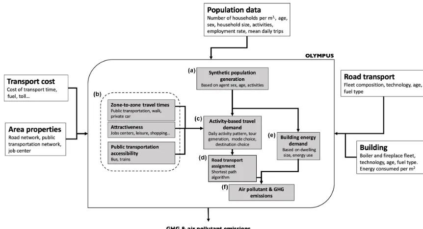
In its current version, OLYMPUS models the main pollu-tant emissions linked with energy consumption, namely road transport and combustion processes from domestic activities and building heating in the tertiary sector. This last sector is composed of activities related to trade and services, but also to information and communication as well as finance. It also includes public administration, education, human health and social action. It will also be referred to as the commercial– institutional sector. As shown in Fig. 1, OLYMPUS is com-posed of six calculation modules supporting four main tasks. The first task of the model is to create a synthetic pop-ulation to which a set of properties will be assigned. This synthetic population is designed to be representative of the population living in the territory concerned and is character-ized by the age, gender and main activity of the agent as well as his or her belonging to a household. The creation of this synthetic population is based on the reconstitution of surveys in the GAIA module (panel a of the flowchart in Fig. 1).
The second task of OLYMPUS is to provide a transporta-tion database built by taking into account the lifestyles of individuals. This database is obtained from successive diag-noses on the generation of individual trips – zonal attractive-ness, spatial and temporal distribution of activities, transport supply, and choice of routes. In the OLYMPUS modeling process, this task is based on three modules.
– A first module, THEMIS (b), defines the accessibility andattractivenessof the different administrative units of the city, as well as the average time travels between them.
– An activity-based travel demand (ABTD) module called MOIRAI (c) computes the daily activity patterns of all agents. It also describes their daily mobility in time and space.
– An assignment module called HERMES (d) provides spatialized daily trips by computing the shortest path between the origin and the destination of a trip (OD ma-trices).
In parallel, OLYMPUS is leading the third task of calcu-lating the energy demand of buildings. To this end, the HES-TIA (e) module calculates the average household energy con-sumption per square meter, the size of dwellings and the city energy mix in order to produce a spatialized energy demand for buildings, including a specific climatic correction on the simulated period.
In the fourth task, OLYMPUS generates emissions from both road transport and small combustion heating systems. These emissions are calculated using reference methodolo-gies such as COPERT IV for road traffic, whose development was ensured by the European Environment Agency (EEA) in the framework of institutional and research activities on air quality and climate. For buildings, emission calculation methodologies are also taken from the EEA guidebook (Eu-ropean Environment Agency, 2013). The computation of pol-lutant emissions is carried out by the VULCAN module (f).
All running OLYMPUS scripts are shell based, Python 2.7 programmed, and C compiled for faster execution speed. For network graphs and spatialized data analysis, NetworkX (Hagberg et al., 2008), as well as GeoPandas and NetCDF, libraries were included in the Python interpreter. Due to the large number of computation loops, the model applies data parallelism that consists of partitioning the data with a multi-threading approach.
3 The synthetic population generator (GAIA)
The GAIA synthetic population generator is the first OLYM-PUS module to be run. It allows for the generation of a syn-thetic population representative of a given urban area. The synthetic population generator uses mainly urban census data to assign each agent in this population an age, gender and main activity, as well as socioeconomic parameters such as possession of a driver’s license. The module distributes this synthetic population over the modeled territory through an urban zoning based on household densities in the urban area – an exogenous variable provided to the model. In the end, we obtain a synthetic population based on census data or demographic scenarios, with an individual description of its agents as the specific contribution of GAIA.
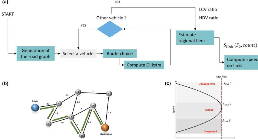
Figure 1.Flowchart showing the OLYMPUS emissions operating system, as well as its main modules.(a)The synthetic population genera-tion module (GAIA).(b)The generator of the transport time matrix, transportation accessibility indices and attractiveness of areas (THEMIS). (c)The transport demand module based on the activity of the synthetic population, and the modal choice in terms of transport (MOIRAI). (d)The module for assigning the travel demand on the road network (HERMES).(e)The module for the generation of energy demand at the regional level.(f)The module for the calculation of greenhouse gas and air pollutant emissions based on emission factors.
must be fed with the total population data and with subto-tals for each of the property types using both aggregated and disaggregated data. Conditional probabilities are also part of the methodologies used to create a synthetic population. This approach is based on Bayesian statistics and relies on a representative sample of population, in which the discrete conditional probabilities governing every characteristic (e.g., age) are identified. Then, a unique value of this characteris-tic is assigned to each agent in the population using a ran-dom distribution that follows the identified probability law. This approach makes it possible to create (on the basis of a representative sample) a database that distinguishes each in-dividual (disaggregated data) as well as each household and dwelling by assigning their own characteristics. These two methods differ in how to generate a built-in population but the results are recognized as quite comparable, although one of the main interests of the IPF procedure is its ability to generate greater variability than conditional probabilities in the population. Despite this, the use of the IPFP in a region such as the Île-de-France would require considerable work to structure the input data. For this reason, we decided to use the conditional probability approach, which has been widely used in the field of transport demand modeling (Antoni et al., 2010; Banos et al., 2010; Mathis et al., 2008). In order to mitigate a possible lack of variability, we implemented a spatial component in the distribution of the socioeconomic characteristics of agents.
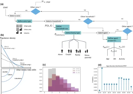
The implementation of GAIA takes place in two main stages and is referenced in Fig. 2.
– The determination of the urban structure is based on an urban density index (UDI) and divided into three classes: the urban pole (CENTER), the urban areas (URBAN) and the suburbs (SUBURBAN) (Fig. 2b).
– For each household in the urban area, the module gener-ates the synthetic population by defining the household size and the properties of the agent using conditional probabilities (Fig. 2).
3.1 Urban structure and population properties
The prerequisites for population generation are the definition of the domain and the classification of urban areas on the ba-sis of an urban density index (UDI). GAIA discretizes the type of urban area on a scale of 1 to 3 (SUBURBAN – UR-BAN – CENTER) according to the population density.
ac-Figure 2. (a)Synthetic population generator GAIA model operating flowchart.(b)Schematic representation of the urban density index (IDU). (c)Example of the household size probability distribution according to a truncated Poisson distribution.(d)Example of a representation of the distribution of the probability of mass function (PMF) of the age of an agent living alone.
cording to the logarithm of population density.
UDI(z)=
CENTER,if log1+nhh
A
>∝2 URBAN, if∝1 <log1+nhh
A
<∝2 SUBURB, if log1+nhh
A
<∝1
, (1)
where ∝1 and ∝2 are key classification values depending on the logarithm of household density,nhhis the number of households,zis a specific area of the domain and Ais the surface area.
Figure 2b shows a schematic representation of the UDI as well as the population-specific attributes for each UDI value. Such discrimination of the properties is necessary for the re-alism of our output data because population density affects the urban landscape (buildings and houses), the location of activities and the structure of households. It is assumed here that the distribution of household types is different between urban centers, surrounding urban areas and suburbs (Pisman et al., 2011; Thomas et al., 2015) and that the distribution of buildings and single-family houses will vary between these different areas. Finally, we have added a variation in house-hold structure with distance from the urban center according to Hulchanski (2010). These hypotheses offer greater
vari-ability in the spatial distribution of agents than a simple con-ditional probability distribution.
3.2 Generation of a synthetic population
The generation of the population depends on probability mass functions (PMFs) that rely on census data, as shown in Fig. 2d, which represent the age-specific PMF of an agent liv-ing alone. In each zone and for each household, GAIA uses a discrete probability distribution to
a. define the number of agents in the household, b. characterize the type of family, and
c. define the gender, age and main activity of agents. Equation (2) predicts the number of agents in the house-hold according to the type of zone (CENTER, URBAN, SUBURBAN), which differ in the density of population and in the distribution of the types of housing. The probability of havingnagents in the household is based on conditional probabilities and defined by a truncated Poisson distribution:
Phhs(n|λ,UDI)=e−λ λn
whereλ is the average household size, nis the number of agents in the household andn∈A, withA=[1, 7] andA∈
N. Figure 2c is an example of a household size probability distribution based on a truncated Poisson’s law.
Equation (3) is used to define the type of household among the four family classes, which are as follows: single (male or female); couple – no children; couple with children; and single-parent family (male or female). The selection of the family type is also based on conditional probabilities (PFAM) and follows
PFAM(n)=
single,ifn=1
P1F(n) ,ifn=2 and ∈R1F
P2F(n) ,ifn≥3 and ∈R2F
, (3)
whereRnFis the family type defined for thenpersons in the household
R1F= {couple,single-parent family}
R2F= {family,single-parent family},
and P1F(n) andP2F(n) correspond to weighted functions based on survey data.
Equation (4) allows us to estimate the attributes of the agents (age, gender, main activity). The gender of each agent is defined by a conditional probability (while the gender of the partner is opposite), such as
Pgdr(η)=
Psex(), if householder and ∈Rgdr
Psex(), if child and ∈Rgdr
Psex2(), if partner and ∈Rgdr
, (4)
whereη represents the situation of the agent in the house-hold,Rgdris the sample space and consists of two elements {male, female},Psex1()corresponds to a weighted function based on the census data and Psex2() is conditioned by the gender of the householder.
The age of an agent depends on the type of household, which is still based on conditional probabilities, and is linked to specific sample spaces: for householders, for couples (age difference less than 20 years) and for children. There are 20 age classes with a 5-year division.
PAGE(η)=
(
PA_1(n) ,if householder and ∈Rhouseholder
PA_2(n) ,if child and ∈Rchild
PA_3(n) ,if partner and ∈Rhouseholder ,
(5) wherePA_1(n),PA_2(n) andPA_3(n) are probability mass functions based on census data. Rhouseholder, Rchild and
Rpartner are age types defined fornpeople in the household with
Rhead= [20;70]andRhead∈N
Rchild= [0;20]andRchild∈N
Rpartner= [20;70]andRpartner∈N.
The principal activity of the agent depends on age and the un-employment rate. Agents under 18 are educated and agents
over 65 are retired. Other agents may be employed, unem-ployed or studying.
PACT(age)=
Pact1(age) ,if 20<age<30 and ∈Ract1
Pact2(age) ,if 30<age<65 and ∈Ract2 school,iffage<18
retired,if age>65
, (6)
wherePact1(age)andPact2(age)represent the mass proba-bility functions giving the probaproba-bility of having as a main activity one of the activities defined inRact1orRact2.
Ract1= {active,school}
Ract2= {active,unemployed}
4 Road transportation generation
To simulate the transportation demand according to the activ-ities of the population, OLYMPUS requires a large number of external data. The spatial distribution of employment centers is a first key parameter: the calculation is based on a spatial-ized file containing the number of jobs per zone, usually in a geographic information system (GIS) format. To simulate ABTD, OLYMPUS uses socioeconomic data at a disaggre-gated level for each area, which this time can be provided by the GAIA synthetic population generator.
Transport networks are a second external parameter needed to calculate mobility. The road network includes ur-ban and nonurur-ban highways as well as major traffic lanes and information on no-load speeds. The public transport network includes all related stations, also in GIS format. All of these data will be analyzed at the finest accessible spatial scale, called the transport analysis zone (TAZ), which can be a dis-trict, a subdisdis-trict, a municipality or any other division of the city. The resolution of the data foreshadows the refinement of the mobility of the population.
The modeling of urban road transport is organized in three stages:
1. determination of the attractiveness and accessibility of the different zones that make up the domain;
2. restitution of the agent travels on the basis of the real-ization of the programmed activities; and
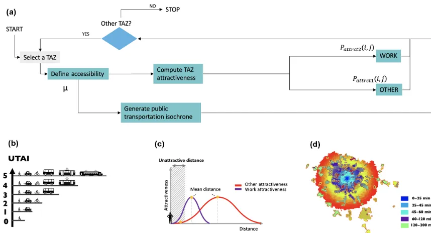
3. assignment of motorized trips on the road network. 4.1 TAZ accessibility and attractiveness (THEMIS) The operating diagram of THEMIS is presented in Fig. 3a. The main steps are
– definition of accessibility and – computation of attractiveness.
mobility choices. Accessibility is calculated from all the ac-tivities considered useful for the agents within a given radius, its value also taking into account the public transport service in this area. For this purpose, THEMIS analyzes the popu-lation density, road network and public transport network of the TAZ. The result is an index with five levels of accessibil-ity accounting for public and individual transport to the area and called the urban transport accessibility index (UTAI).
This flag is used to set the access mode shares. As shown in Fig. 3b, an area with a UTAIMIN will only be accessi-ble by walking (WALK), while an area characterized by a UTAIMAXwill be well serviced with a wide choice of trans-port infrastructure. The definition of the five UTAI classes depends on the value ofµ, defined by the following equa-tion:
UTAI(zone)=
1, ifµ <∝1 2, if∝1< µ <∝2 3, if∝1< µ <∝3 4, if∝1< µ <∝4 5, ifµ >∝4
, (7)
with
µ=log
1+nhh×nst
A
,
where ∝1,∝2,∝3 and∝4 are key classification values de-pending on the logarithm of household density and public transport density.nhhis the number of households per TAZ,
nstis the number of public transportation stations in the TAZ andAis the area of the TAZ. The UTAI (see correspondence in Fig. 3b) thus helps to design the use of the city from its transport infrastructure and to define a realistic travel time for public transport, as represented on the isochronous curve of public transport in Paris (Fig. 3c).
The attractiveness of activities is an important parameter that shapes the agenda of agents. It can be defined as the ability of a zone to get an agent to carry out a given activity on the site, respecting the average length of the trip associ-ated with this type of activity, as illustrassoci-ated in Fig. 3c. The model assumes that there are two types of activities: WORK and OTHER. The complete list of OTHER activities taken into account in the ABTD model are the following.
– HOME – SCHOOL – SHOPPING – SECONDARY – ACCOMPANYING – VISIT – LEISURE
The main parameter that differentiates our two types of activities is the average duration of the journey, which varies considerably, with the average distance traveled for commut-ing (home–work) becommut-ing longer than that of other types of ac-tivities. The distance to the TAZ is an important variable in the estimation of its attractiveness for an agent. The attrac-tion potential of WORK depends on the number of jobs in the TAZ. For OTHER activities, their attractiveness depends on the population density of TAZ. However, some activities like visiting a friend or going on vacation are still underestimated by the ABTD model. The computation of attractiveness is based on Huff’s theory of the gravity model (Huff, 1964). It is based on the definition of an activity weight and works by analogy with Newton’s law of gravity. The probability of conducting any activity at a specific location is therefore de-fined as follows:
P(i,j)=
(i, j, d)
P
j(i, j, d)
, (8)
where the attractivenessis defined by
(i, j, d)=X iAct×
X
jAct×
1
σ
√ 2πe
−1 2(
|x−d|
σ )
(9)
andσ=d 2.
In this equation, dmean represents the average distance to reach the activity, whilei andj are the indexes of the ori-gin and destination zones, respectively.
In the end, the attractiveness parameter is highly depen-dent on the city’s structure and the travel practices of the inhabitants. Kwan and Weber (2003) found that few people act to minimize their commute to work by relocating their home or workplaces. Given this, mobility surveys provided by some countries can be used to force average travel dis-tances and make them more realistic.
4.2 Activity-based travel demand (MOIRAI)
Figure 3. (a)The transport time matrix generator, transportation accessibility indices in common and attractiveness of zones of displacements (THEMIS) flow diagram.(b)Schematic representation of UTAI.(c)Schematic representation of the attractiveness of an activity towards an individual as a function of distance.(d)Example of isochronous transit curves from the center of Paris.
hypothesis on which the choice is based is that the maximiza-tion of utility influences the decisions of the agent. MOIRAI relies on the use of the multinomial logit (MNL) model (Mc-Fadden, 1973) in which the random components of utility are considered independent, identically distributed (IID) and follow a Gumbel distribution:
Pmode,i=
e−Utilitymode,i Pn
i=0e
−Utilitymode,i, (10)
where Utilitymode,i represents the utility function of a
trans-portation modei.
MOIRAI is implemented in three main stages common to many ABTD models (Castiglione et al., 2015):
2.1 generate the daily activities of the agent (number of trips and tour sequence),
2.2 agent schedule management (duration of activities), and 2.3 identify the type of transportation used for each trip
(lo-cation and modal choice).
These steps are described in the MOIRAI operating dia-gram in Fig. 4a.
4.2.1 Generation of daily activities
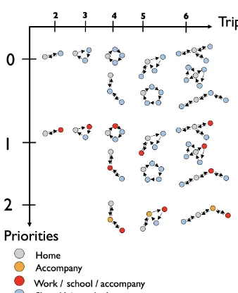
An important step in modeling an agent’s schedule is the es-timation of the number of trips the agent makes during the day, as shown in Fig. 4b. A first step in the simulation of the agent’s agenda is therefore to define priorities. The obligation
to conduct an activity – such as going to work or accompa-nying children for care or education – defines the priority of an officer. Once these priorities are set, an agent can perform optional activities such as shopping, visiting a friend or going to the movies. There are three priorities in the model: work – school – accompanying (bring a child under 10 to school). The model can combine the priorities of the work and ac-companying activities. The number of trips per day (p) per-formed by an agent depends on priorities (x) and is based on the following discrete probability distribution:
Ptrips(x)=
Ptrips act1(x) ,if priorities=1
Ptrips act2(x) ,if priorities=2
Ptrips other(x) ,if priorities=0
Ptrips retired(x) , if agent age>65
, (11)
where Ptrips act1(x), Ptrips act2(x), Ptrips other(x) and
Ptrips retired(x) represent the probability of performing
p daily trips according to thex priorities of the agent and withx, p∈N.
Figure 4. (a)The transport demand module MOIRAI operating flow diagram.(b)Representation of a circuit of activities of an agent of the synthetic population.(c)Representation of the timetable of an agent of the synthetic population.(d)Representation of the probability of favoring a mode of transport according to the cost of transport time.
Figure 5.The transport demand module MOIRAI activities circuit based on agent priorities and daily number of trips (p).
home-based sequence, MHBS) or be fully performed without returning home (nonhome-based sequence, NHABS). Fig-ure 5 shows the different types of sequencing modeled in OLYMPUS. Depending on the number of trips, it is possible to create a single home circuit or several circuits, one cen-tered on the place of residence and others on the activities. The probability of making one or more circuits depends on the number of daily trips.
After generating the agent schedule, the module locates each activity. Depending on the TAZ in which the agent is located, the model estimates where the agent will have the highest probability of carrying out the planned activities. This is done according to the attractiveness of the TAZ cal-culated by THEMIS and by using Huff’s random probability approach for choosing the place of activity. For the location of the WORK activity, we use theP(i,j)probability of attractiveness of the employment center. For OTHER activ-ities, theP(i,j)probability of attractiveness is based on population density.
The last step in the generation of daily activities is the insertion of the time of realization of the activities, which requires the attribution of a duration to each of the actions carried out by the agent. As shown in Fig. 4c. MOIRAI cal-culates this parameter using conditional probabilities with a time step of 1 h. The module assigns a random value to the start time based on the agent’s priorities. If the sum of the activities exceeds 24 h, the simulation is restarted.
For the first activity, the start time is calculated as follows:
ACTst1(act)=
stescort(x) ,if act=escort stschool(x) , if Act=school stwork(x) ,if act=work stother(x) ,if act=other
, (12)
where
itime(i)=Xi−1
0 DurAct(j )+ACT st
1(Act) (14)
and Dur represent the duration of activities, defined as a ran-dom variable in a truncated interval over a time range. The distribution of start time and duration of activities in OLYM-PUS is presented in Fig. 6.
4.2.2 Modal split
The modal choice is clearly a critical parameter for calculat-ing pollutant emissions from urban mobility. In OLYMPUS, travel modes include WALK (walking and cycling), PC (pas-senger car and two-wheeled car) and PT (public transport in-cluding metro, bus, tram and train). The objective is to define the probability of using a specific mode of transport accord-ing to their utility for a given route and agent. The modal choice is obtained from the expression of the utility function for each transportation mode (Umod,i). The value of utility
comes from a cost calculation including the generalized cost of transport (including the time budget (tbudget), the percep-tionaof modeiand the monetary cost (mcost)). In this calcu-lation, the travel time can be penalized by different elements of the trip such as tolls, congestion and parking problems in-cluded in the variablePmod:
Umod,i=mcost+a·tbudget+Pmod. (15) The utility function of the WALK mode mainly depends on the time cost of the trip. The WALK mode average speed, SpeedWALK mean, is defined to be 3.6 km h−1. Thus,
Umod,WALK=
ODdistance
SpeedWALK mean+PWALK, (16) wherePWALKrepresents walk penalties, and the distance be-tween the origin and the destination activity, ODdistance, is based on the great-circle distance calculation,
ODd=Arccos(sinϕA×sinϕB+cosϕA×cosϕB×dλ), (17) where A and B respectively denote the origin and destina-tion points,ϕA,ϕB,λA andλBrepresent their latitudes and longitudes, and dλ=λB–λA.
For the individual passenger car mode (PC), the utility function is defined as follows:
Umod,PC=
ODdistance
SpeedPC mean +CostCAR+PPC. (18) By default, the average speed of PC mode, SpeedPC mean, is set to 22.6 km h−1 in urban areas. This value is based on Hickman et al. (1999) and represents the average driving speed in urban areas recorded during the MEET project. The ODdistanceis also based on the great-circle distance equation (Eq. 17).
The CostCAR variable represents the average kilometric cost of the use of a private car. All penalties are coded as additional monetary costs: these include tolls, parking tick-ets, congestion and taxes as well as additional penalties for short-distance trips. All of them can be summed in the cal-culation of PC mode utility. The time cost for the agent is calculated from the shortest path. This step of OLYMPUS requires considerable computation time because of the large number of agents.
With regard to the utility function of public transport (PT) from one TAZ to another, we use the following equation:
Umod,PT=tPT+CostPT+PPT. (19) In this equation, the travel time with PT mode is TimePT. It depends both on the accessibility of the destination area and the average distance between origin and destination points. The average travel time from one TAZ to another includes the duration of walking, waiting and traveling. It is calculated using a linear regression based on time zone transport survey data and is therefore based on realistic values.
tPT(d, z)=αi,j×a×d+b+WTime(UTAI), (20) whereαi,j represents the average transit time between two
zones and a and b are the linear regression coefficients.
WTimeis the UTAI-dependent waiting time.
ThetPTparameter is usually calculated using general tran-sit feed specification (GTFS) data, if available for the city, and computed using either the connection scan algorithm (Dibbelt et al., 2013) or the RAPTOR algorithm (Delling et al., 2012). The limitation of these methods is the huge com-puting time required. As a consequence, they were not cho-sen here. Since public transport time is an escho-sential variable for the estimation of the general cost of public transport, we have developed a methodology based on a zonal approach and using the UTAI. This method has limitations with respect to CSA or RAPTOR algorithms. However, we consider that a realistic simulation of the UTAI matrix and an appropriate calibration of the module with real transport times can lead to satisfactory results. The CostPTvariable represents the daily cost of transit. Transit penalties may be well represented by the frequency of transit service.
4.3 Assignment
The transport demand previously generated by the ABTD module MOIRAI generates travel matrices providing infor-mation only about the origins and destinations of the flows. The next step is to project on our modeling grid the paths taken by the agents in order to provide spatialized pollutant emissions from transport. For this purpose, we only take into account flows related to private vehicle use.
Figure 6.Distribution of activity start times and individual time spent on an activity.
VISSIM (Gomes and May, 2004), AIMSUN (Barcelo et al., 1989) and PARAMICS (Cameron et al., 1994). A second ap-proach is that of mesoscopic models, which are interested in the evolution of sets of vehicles, like the models CON-TRAM (Taylor, 2003) and DYNASMART (Mahmassani et al., 2005). Both approaches are not very compatible with the scale of the city, on which we focus. Indeed, although the use of instant-emission models like PHEM (Rexeis et al., 2013) and MOVES (U.S. Environmental Protection Agency, 2013) can provide added value, obtaining input traffic data describ-ing each cycle of acceleration and deceleration of the vehicle is quite difficult, and their consideration requires high com-putational time. These constraints make the microscopic ap-proach somewhat precarious. We must therefore rely on a macroscopic description of the traffic in the form of a vehi-cle flow and using global variables such as the average speed on each section of a traffic axis, as in the DAVISUM (Bro-quereau, 1999) and TransCAD (Caliper Corporation, 2010) models. As most of these transport models are not open source, we opted for the development of our own traffic as-signment model within the OLYMPUS ensemble: HERMES. HERMES is a macroscopic traffic module that works with average speed values for vehicle flows, ignoring the dynam-ics of traffic on a road. This approach is compatible with our simulation scale. It is also compatible with the most common methods of estimating traffic-related combustion emissions,
which rely on emission factors per driving cycle, each cycle being characterized by an environment (city, highway, etc.) and by a mean speed per strand.
The HERMES module consists of four main stages in the assignment of agents to the road network (See Fig. 7a).
3.1 Definition of the road graph. The road network is ex-tracted from GIS road data and transformed into a graph that records the connections between different road sec-tions, thus creating a set of edges and nodes (intersec-tions) using the graph theory (Bondy and Murty, 1982). The speed limit is the main attribute of edges.
3.2 OD shortest path. HERMES computes the shortest path for each trip by solving Dijkstra’s algorithm (Dijkstra, 1959). For each trip, the module identifies the nodes of the graph closest to the georeferenced O and D points. To choose the shortest path among the algorithm out-puts, HERMES uses the time spent on a link as weight-ing.
vehi-Figure 7. (a)Operating diagram of the assignment of transport demand on a road network (HERMES).(b)Representation of the calculation of the shortest path based on the speeds of road sections.(c)Speed flow curve of the MOIRAI module based on three levels of road saturation.
cles (HDVs) and light commercial vehicles (LCVs) are therefore not taken into account. This is why we devel-oped an approach that extrapolates the transportation of goods and interregional transportation trips based on a reference ratio of passenger cars to total fleet and us-ing ratios between HDV and LCV in urban areas. In-deed, fleet composition surveys are available for many cities. They are often based on transport organizations like TFL in London.
3.4 Speed on link computation. Finally, HERMES inte-grates network congestion in its assessment of mobil-ity. Road congestion alters speed on the road network as shown in Fig. 7c. The approach is based on the UK Department of Transport (1997) and can be represented as follows:
Slink=
S0,ifFi<50
S0−
S0−Sc
Fc−F0
×(Fi−F0) ,ifF0< Fi< Fc
Sc
h
1+ Sc
8×d
×Fi
Fc−1
i,ifFi> Fc
, (21)
where the speed on the road link Slink depends on the flowFiand lengthd.S0is the free-flow speed,Scis the congested speed, andFcis the road link flow capacity. This is one of the approaches suggested by Ortuzar and Willumsen (2011) to attempt to represent empirical conges-tion. One of the limitations of this methodology is the con-sideration of the impact of signaling. Other congestion func-tions such as that presented by Akçelik (1991) make it possi-ble to better manage delays at junctions. On the other hand,
this method requires knowledge of the location of the traf-fic lights. For street-level studies, the Akçelik (1991) method adds a certain realism to traffic modeling. However, it has been shown that the approach we have chosen produces a satisfactory estimate of traffic flows and road network satu-ration on the main roads.
5 Building energy demand
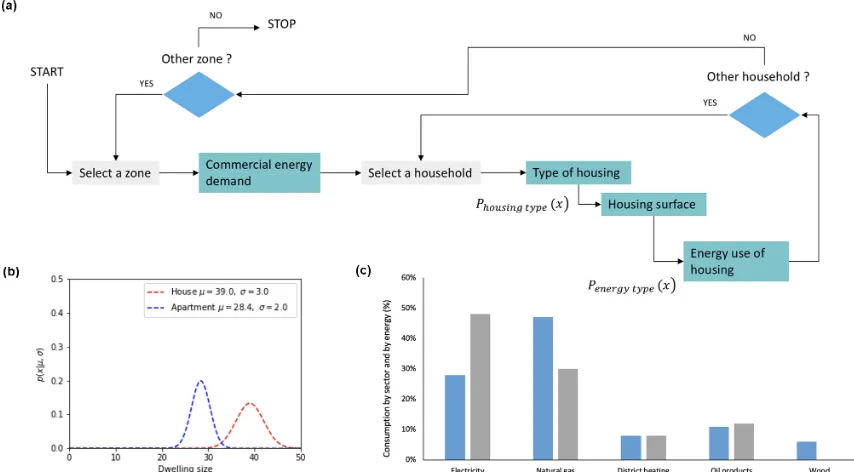
Figure 8 shows the organizational chart of HESTIA, the OLYMPUS module responsible for simulating the energy de-mand of a building. HESTIA uses the type of dwelling, the living space of the household and its average annual energy consumption as input parameters. The main task of this mod-ule is to spatialize the energy demand in the territory.
mod-Figure 8. (a)Energy demand in the regional level generator (HESTIA) flow diagram,(b)example of dwelling size distribution and(c) prob-ability mass function of the type of energy consumed for different types of dwellings.
ule. It lists combustion activities for residential, institutional and commercial heating, as well as domestic hot water and cooking. The process is similar to top-down approaches, but the implementation of bottom-up factors related to energy efficiency or household characteristics makes it possible to consider the implementation of energy scenarios.
The generation of energy demand in the residential sector is achieved by modeling the energy demand of each house-hold. It depends on the size of the household, the size of the dwelling, the type of housing, the age of the dwelling and a coefficient of thermal efficiency. To generate the energy de-mand of the residential sector, HESTIA uses population den-sity. The first step is to determine the ratio of collective hous-ing to individual houshous-ing accordhous-ing to the population density and type of area using GAIA outputs. This ratio is clearly dependent on the country and local data such as building heights or urban density. The calculation must therefore be specific to the area of interest. In HESTIA, the distribution of household dwellings (house or apartment) is formulated as follows:
PDW type(x)=
PDW urb(x) , if zone=urban
PDW sub(x) ,if zone=suburban
PDW rur(x) , if zone=rural
. (22)
We assume that the CENTER and URBAN areas com-prise a majority of buildings, while the SUBURBAN areas are where most of the individual houses are built. First of all, HESTIA starts by calculating the size of the dwelling (DWzone) according to a reference size value for different type of dwellings (SurfHT), which depends on each specific
zone (γUDI) and takes into account the number of agents (n) living in the dwelling:
DWzone=SurfHT×γUDI×n. (23)
The energy used to heat and boil water is defined by the dis-tribution of the energy mix, an exogenous parameter in the model:
Penergy=
P energy1, if house
P energy2, if apartment. (24) Then, HESTIA calculates the energy consumption per house-hold, ENcons, taking into account the size of the dwelling, DWzone, the unit energy consumption per household (ECU) and the household size (hhsz):
ENcons(hh)=DWzone×ECU×hhsz. (25) Finally, the module applies a climatic correction to energy consumption in order to estimate the underconsumption or overconsumption of energy due to the cold or hot climate. The degree-day (DD) is the parameter allowing us to quan-tify this correction as a function of the daily temperature of the considered year compared to a reference year (Jones and Harp, 1982).
Thus, the energy demand of employees can be defined as ENWcons(employee)=ECUw×nworker. (26) A climate correction is also added to the consumption of this sector.
6 Emissions
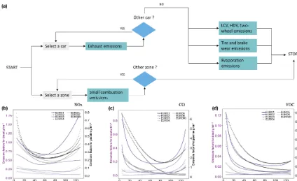
The role of the VULCAN module is to calculate pollu-tant emissions from both road transport and the energy con-sumption of buildings, which is the final step of OLYM-PUS. There, the quantification of pollutant emissions is based on methodologies recommended by the European En-vironment Agency (EEA) guidebook for air pollutants and greenhouse gas (GHG) emissions (European Environment Agency, 2013). They rely on the use of emissions factors, which may depend on the type of fuel, but also on the age and combustion technology of the engines and stoves. The organizational chart of VULCAN is shown in Fig. 9a. 6.1 Road emissions
Road transport emissions – referred to as mobile emissions in the inventory – are calculated on linear road sections where traffic properties at a given time are homogeneous (driv-ing cycle, average speed). For passenger vehicles, the traffic flows are derived from the travel matrices of the assignment module. From a quantitative point of view, emission factors based on traffic characteristics are applied to each section of road in order to obtain the quantities of pollutants emitted into the atmosphere per unit of time. In the literature, three main databases provide exhaust emission factors. These are HBEFA (Keller et al., 2017), COPERT (Ntziachristos et al., 2009) and MOBILE6 (US EPA, 2003). They differ in that some depend on instantaneous speeds, while others consider average driving speeds or apply to specific driving cycles such as standard highway traffic. The methodology we de-veloped for the VULCAN emissions module is based on the recommendations of the EEA, which use COPERT emission factors based on the average speed of a vehicle during a stan-dard driving cycle (see Fig. 9b, c, d). To be comprehensive in the counting of traffic-related emissions, we added the me-chanical emission of particles from different forms of fric-tion and abrasion during driving, as well as the evaporafric-tion of NMVOC from vehicle tanks.
A critical step in the road transport emissions modeling process is to determine the composition of the fleet, which can be inferred from the national composition data as exoge-nous data. In the assignment module, the choice of specific emission factors depends on the properties of the fleet (age, cylinder, fuel type), and the properties of the agent’s car are defined using a conditional probability law. A second impor-tant step is the addition of cold-start emissions. This makes it possible to take into account the over-emission effect re-sulting from the poor performance of a vehicle starting and
then running with a low-temperature engine. In order to ob-tain total exhaust emissions, VULCAN first calculates hot emissions factors for the stable engine regimes:
Ehot=N×M×εhot, (27) whereN is the number of cars on a road link,Mis the length of the road link andεhotis the emission factor. Then, VUL-CAN calculates cold-start emissions using an over-emission factor applied to a fraction of the distance traveled by each vehicle. This factor can be defined as
Ecold=β×N×M×εhot×
εcold hot
−1, (28)
whereβ is the average fraction of the total distance traveled with a cold engine, andεcold
hot is the cold-to-hot ratio. The cal-culation algorithm of the cold–hot emission quotient strongly depends on European technology, on the ambient tempera-ture and on the pollutant being considered (European Envi-ronment Agency, 2013).
The EEA offers several levels of refinement of calcula-tions, called Tiers, the use of which depends on the informa-tion available at the input of the calculainforma-tion. Tier 1 methods are based on a simple linear relationship between activity data and emission factors representing typical or averaged process conditions, which tend to be technology indepen-dent. More advanced Tier 2 methods are available for key categories, allowing us in particular to apply country-specific emission factors that depend on processing conditions, fuel qualities or abatement technologies (European Environment Agency, 2013). OLYMPUS uses the highest level of acces-sible detail each time. All emissions are then computed as follows:
Etieri =N×M×εtieri, (29)
whereM is the number of traveled kilometers. For exam-ple, the calculation of emissions from LCVs, HDVs and two-wheeled vehicles is based on the EEA Tier 2 method. This methodology is used because of the excessive uncertainty of the freight fleet. HERMES generates the numberN of ve-hicles using standard fleet composition ratios. Emissions are calculated for CORINAIR pollutants (NOx, NMVOCs, PM)
and for CO2.
As mentioned above, emissions related to tire and brake wear add to exhaust emissions according to the following two equations (European Environment Agency, 2013):
Etire=N×M×εTSP×fs×Ss(V ), (30)
Ewear=N×M×εTSP×fs, (31) whereεTSPis the mass emission factor of total suspended particulate matter (TSP) for vehicles in categoryj (g km−1),
Figure 9. (a)Greenhouse gas and air pollutant emissions module (VULCAN) flow diagram;(b),(c)and(d)represent NOx, CO and NMVOC
emissions factors from diesel and gasoline passenger cars.
Finally, the VULCAN module considers the evaporation of gasoline using the following equation (European Environ-ment Agency, 2013):
Eevap= X
N×εevap×365, (32) whereεevapis the evaporative emission factor depending on the ambient temperature.
6.2 Building emissions
Emissions from buildings are based on the EEA guide-book for small combustion emissions (European Environ-ment Agency, 2013). This part of the VULCAN module takes into account emissions from residential heating (fireplace, stoves, cookers, small boilers), as well as institutional and commercial heating. Small combustion emissions from the agricultural sector are not considered.
The calculation of residential and commercial– institutional emissions is based on the EEA methodology and emissions factors derived from Pfeiffer et al. (2000) and Kubica et al. (2007):
Ebuilding= X
fuel(εfuel×ENcons(hh)). (33) There are several types of heating and boiling equipment to consider in combustion modeling for the residential, com-mercial and institutional sectors (fireplaces, stoves, cookers, small boilers, space heaters, combined heat and power on a small scale). It is important to note that the composition and
the age of the fleet are two crucial parameters affecting the emissions of a building, as emission factors vary with equip-ment and age. It has been found that improved combustion technology has a significant impact on pollutant emissions over the years. However, due to a lack of information in the literature, these parameters remain difficult to estimate ac-curately. For these reasons, when applying OLYMPUS to a territory, the hypotheses that we will be able to propose for the partition and the spatial distribution of the technologies of heating systems will be a determining point for the realism of the simulation.
7 Application to greater Paris
area, the quality of the available input data would allow for greater robustness and better reliability of the simulations.
We conducted a 1-year simulation with OLYMPUS in the Paris region. The input data selection, working assumptions and configurations selected for the OLYMPUS model are described below. The results of the emissions calculations are then analyzed. The source code can be obtained from the LISA website at http://www.lisa.u-pec.fr/~aelessa/OLP (Elessa Etuman, 2018) or upon request to the authors. 7.1 Configuration
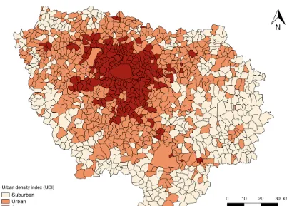
The simulations were carried out for the year 2009, for which we had a large database of input data (surveys, censuses, in-ventories). The simulation domain is the Île-de-France region (greater Paris). It is a monocentric urban area with a popula-tion density of 21 000 inhabitants km−2in the city center and a density that decreases radially to the remote suburbs, which are predominantly rural (Fig. 10).
The population in this territory is greater than 11 million inhabitants. In terms of transport infrastructure, Paris is con-sidered by the Institute for Transportation and Development Policy as the city with the most efficient network (Marks, 2016). Individual mobility is 3.87 trips per person per day on average, with 41 million trips made each day in the region. The majority of trips (70 %) do not include travel to the cen-ter of the metropolis: trips in Île-de-France are mostly short (4.4 km on average) and close to home.
In OLYMPUS, the computing space unit is TAZ. Here, it comes from the National Institute of Statistics (INSEE), which has set up a specific division of the territory called IRIS that gathers between 1800 and 5000 inhabitants. For our domain, this choice leads to the constitution of 1300 TAZs. Figure 11 illustrates the division of the region into IRIS, as used by OLYMPUS.
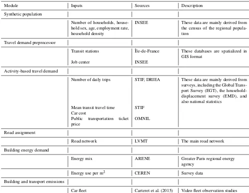
The modeling of anthropogenic combustion emissions resulting from individual activities requires a very large amount of data. The main sources of these data are shown in Table 1. To generate the synthetic population in GAIA, we used aggregated data from the census of the city, mainly derived from INSEE. They include the distribution of the population in the territory by age and gender, the number of households by IRIS, and the average distribution of house-holds by type (single, couples, family, single-parent family). Mobility calculations in MOIRAI are based on several types of data, mainly surveys or national statistical databases. First, the accessibility of the area by public transport was assessed on the basis of the density of the public transport networks provided by the STIF regional transport agency. Regarding the attractiveness of urban subareas, the creation of attractive WORK zones is based on INSEE census data, which provide the number of jobs per municipality. The average distance at which agents can be attracted to an occupational zone is then deduced from the city’s overall transport survey (STIF, 2012). The total mobility of the agents is also conditioned by
the total number of trips per day weighted according to the number of priorities of the agents. Here, the average number of daily trips was estimated from local surveys, and we as-sumed that trips other than those related to commuting were characterized by the same average distance, which is not the case in reality. For the OTHERS category, agent interest in a given activity results from two main parameters: the num-ber of households in the immediate vicinity of an activity and the estimated average distance traveled to reach this ac-tivity. Once these values are set, the determining parameter for carrying out the activity will be the estimated duration of the trip. Here, this parameter was derived from THEMIS, whose calibration had been achieved through an online ap-plication based on GTFS data from all regional transport agencies. It allows for the constitution of a matrix of average transport times between the different classes of urbanized ar-eas (UTAI). In the end, the combination of transport network data and population density makes it possible to calculate the accessibility of any area of activity.
The fleet of vehicles used in HERMES dates back to 2009 and is based on the Carteret et al. (2015) survey. It includes passenger cars, LCVs and HDVs. This study is based on the use of video observation to characterize a fleet of vehicles, then comparing to the global transport survey. The regional fleet of stoves and fireplaces was not estimated, so it was not included. We simply assumed here that individual heat-ing modes, includheat-ing wood heatheat-ing, came mainly from indi-vidual dwellings. The total energy demand in the territory was estimated from data from ARENE surveys (Regional Agency for the Environment and New Energies) providing unitary consumption of households in Île-de-France, but also from information on the average household housing area, by type of household and by place of residence, provided by CEREN (Center for Economic Research on Energy). The consumption modeling of the commercial–institutional sec-tor was carried out on the basis of annual consumption per employee in the commercial–institutional sector (CEREN, 2015).
7.2 Results and discussion
Figure 10. (a)Representation of the Île-de-France region (greater Paris) and the land use.(b)Representation of the Île-de-France subdivision.
Table 1.OLYMPUS parameterization for the greater Paris simulation.
Module Inputs Sources Description
Synthetic population
Number of households, house-hold sex, age, employment rate, household density
INSEE These data are mainly derived from the census of the regional popula-tion
Travel demand preprocessor
Transit stations Île-de-France These databases are spatialized in GIS format
Job center INSEE
Activity-based travel demand
Number of daily trips STIF, DRIEA These data are mainly derived from surveys, including the Global Trans-port Survey (EGT), the household-displacement survey (EMD), and also national statistics
Mean transit travel time STIF Car cost
Public transportation ticket price
OMNIL
Road assignment
Road network LVMT The main road network
Building energy demand
Energy mix ARENE Greater Paris regional energy
agency
Energy use per m2 CEREN Survey data
Building and transport emissions
Car fleet Carteret et al. (2015) Video fleet observation studies
the labor force, we consider the model to generate an accept-able synthetic population for transport modeling. Finally, the average attributes of the agents used as forcing in an aggre-gated form are correctly represented in the synthetic popula-tion: gender data, unemployment rate, distribution of house-hold types and average househouse-hold size. Because OLYMPUS relies on Bayesian statistics to generate a synthetic popula-tion, to obtain representative results it is necessary to ini-tially have a large database containing specific information on the distribution of agent characteristics in the population. Thus, thanks to the transcription of stochastic variables, the synthetic population has great similarities with the popula-tion studied. Nevertheless, this approach produces limited variability in socioeconomic parameters within the distribu-tion, offering a simulated population too close to the average characteristics of the actual population. In this simulation, we limited ourselves to the use of a three-level UDI and the division of the domain into 1300 TAZ. In order to define the most sensitive components of the urban system modeled with
OLYMPUS, it will be interesting to test the sensitivity of the outputs of the model to the increase in the spatial variability of the properties of the agents, to the use of a wider range of indices and to a greater number of TAZs.
Figure 12. (a)Representation of all origin–destination flows generated by MOIRAI motion request module.(b)Representation of daily road traffic in greater Paris in terms of volume over capacity (VOC),(d)nitrogen oxide emissions in Île-de-France from road transport and residential–commercial–institutional sector (OLYMPUS),(e)focus on emissions from road transport,(f)focus on emissions from the residential–commercial–institutional sector.
survey-based data on average number and length of trips per day. The simulated data are very realistic, with a difference of only 4 % for the total number of trips per day and per agent in Île-de-France and an overestimate of 6.9 % for the average trip length compared to average values of the trans-port survey. The total number of trips and the modal shares are very close to reality (less than 3 % difference with field data). If we consider differences of less than 5 % between simulated and observed values to be satisfactory and differ-ences of less than 3 % to be very satisfactory, then this first comparison work reveals that OLYMPUS simulates the main characteristics of regional transport demand satisfactorily to very satisfactorily. Only the simulated average trip length is not completely satisfactory (+6.9 %). In order to evaluate the OLYMPUS results in more detail (and to propose a compre-hensive correction of the average trip length), future works could include a map of the simulated and observed mobility. This spatialized analysis would take into account the frac-tion, length and the modal share of the trips made between the different zones (center to center, center to near suburbs, suburb to suburb). Such an evaluation requires a lot of data to be processed, but it could allow for both a more refined evaluation of OLYMPUS outputs and a diagnosis of mobil-ity levers in the model.
Figure 12c shows a map of simulated energy demand in greater Paris. The results show a fairly logical positive
de-Table 2.Comparison of mobility with global transport surveys.
OLYMPUS OMNIL RD
Average number of trips per day 4.05 3.87 4.6 % Average length of a trip (km) 4.7 4.4 6.9 % Total number of trips (millions) 41 41 1 % Motorized individual trips 40.4 % 39.5 % +0.9 % Walking, cycling 41.9 % 40.3 % +1.6% Trips by public transportation 17.7 % 20.1 % −2.4 %
pendence on the total population, with maximum demand at the center of the agglomeration. The total energy consump-tion of greater Paris (including energy demand for electricity) was 303 TWh in 2009 according to ARENE (2013). The en-ergy consumption from the residential, commercial and insti-tutional sectors represents more than 50 % of this total. The modeling of the regional energy demand (HESTIA) is con-sistent with surveys, the difference being around+9.6 %.
com-bustion processes, show very good consistency with the spa-tial emitting patterns in Île-de-France (major roads, types and density of housing by zone). The total emissions of OLYM-PUS are then compared to two reference emission invento-ries: the AIRPARIF air quality network inventory and that of the European network EMEP. To this end, we have ex-tracted for each inventory the activity sectors corresponding to the emissions calculated by OLYMPUS. The comparison is presented as histograms in Fig. 13 for NOx and for two
size sections of particulate matter: PM2.5and PM10. It should be noted that the calculation methods differ between the two “reference” inventories: AIRPARIF develops bottom-up ap-proaches from local data collection, while EMEP inventories are derived from national totals by species, which are spa-tially disaggregated using top-down approaches. In addition, the comparison with the EMEP inventory cannot be done in detail due to the lack of information on the subsectors of ac-tivity in the EMEP data.
The emissions produced by OLYMPUS, although slightly underestimated compared with the emissions of AIRPARIF, are considered here as very satisfactory. Indeed, the OLYM-PUS emissions, either total or by vehicle type, show differ-ences of less than 20 % with the AIRPARIF values for nitro-gen oxides (NOx) and particulate matter (PM2.5and PM10). The variations in the AIRPARIF emissions from one sub-group to another (PC, LCVs, HDVs) is also reproduced well by OLYMPUS. This is remarkable considering that OLYM-PUS (which constructs mobility matrices using a gravity ap-proach and relying on the choice of individuals) has very few forcing data in common with AIRPARIF (which mainly uses road count data, vehicle sales and registration, fuel con-sumption surveys). In particular, although both inventories use the COPERT methodology, other sources of differences exist, notably in the hypotheses about the fleet in circulation. An earlier study by Timmermans et al. (2013) confirms that the observed discrepancies in emissions are consistent with the fact that different approaches are used. Indeed, the au-thors indicate that the expected gap between emission inven-tories based on different modeling assumptions (choices on the cold-start fraction, fuel evaporation emissions modeling, engine fleet) is expected to be 20 % at the minimum. By con-trast, particulate matter emissions related to abrasion seem to be more severely underestimated by OLYMPUS compared with the AIRPARIF database (−30 %), but there are cur-rently very few ways to estimate real emission values. De-viations from the EMEP inventory are greater, which can be explained by the fact that the EMEP approach is coarse and strongly overestimates some emissions compared with the AIRPARIF inventory. Nevertheless, the tendency to un-derestimate emissions in OLYMPUS may reflect the lack of consideration of specific sources in the model. In particular, the model calculates the transport of goods on the basis of occupancy rates on urban roads and does not take into ac-count interregional mobility, the city being considered here as a closed system. This largely explains the underestimation
of traffic at the borders of the region and in certain rural areas (not shown here). Taking this source into account is consid-ered as a priority evolution of the model.
In addition, the issue of congestion should not be treated superficially in a model like OLYMPUS because it affects the decision of the agents along their commute and contributes to an increase in emissions. At present, congestion is man-aged by the representation of speed classes on the main axes, but more dynamic management of this process is envisaged. One of the methods identified to address this problem is the establishment of an iterative process between congestion and the choice of agents and the refinement of the representation of speed as a function of the occupancy rate of the lanes. This is also what future developments of the platform will focus on.
The activity sector that shows the highest differences be-tween the two regional inventories is residential combustion, with OLYMPUS underestimating the value of the AIRPARIF inventory for PM10 by a factor of 2. However, we men-tioned that we do not have information about local combus-tion equipment data and that equipment technology is a de-terminant factor of emissions related to heating. In particular, wood burning is responsible for more than 90 % of particu-late matter emissions in this sector. In addition, AIRPARIF has its own modeling assumptions for residential heating, in-cluding industrial heaters not based on local data, as well as an estimate of the number of chimneys and stoves. Further-more, there is no specific survey on combustion technolo-gies in the commercial and institutional sectors. This point explains the very large variability of emission estimates in the different inventories. The comparison between invento-ries can hardly overcome this lack of constraints. We should therefore consider the range of values given by OLYMPUS to be consistent with the estimates of the reference inventories, and our work contributes to the improvement of the evalua-tion of household combusevalua-tion emissions in Île-de-France.
Finally, as for the total number of trips, the structure of trips and the modal share, the results simulated by OLYM-PUS are quite close to the data used as a reference (surveys or models), which validates each of the steps in OLYMPUS: the representation of the average number of trips per agent, the division of urban areas into attractiveness classes and the use of the utility function for modal choices. As a conse-quence, our modeling approach appears relevant for analyz-ing the links between city, population, mobility, energy con-sumption and pollutant emissions. A better consideration of the effects of freight transport and congestion will make anal-yses conducted with OLYMPUS even more robust.