Variational Particle Approximations
Ardavan Saeedi* [email protected]
Computer Science & Artificial Intelligence Laboratory Massachusetts Institute of Technology
Cambridge, MA 02139, USA
Tejas D. Kulkarni* [email protected]
DeepMind, London
Vikash K. Mansinghka [email protected]
Department of Brain & Cognitive Sciences Massachusetts Institute of Technology Cambridge, MA 02139, USA
Samuel J. Gershman [email protected]
Department of Psychology and Center for Brain Science Harvard University
Cambridge, MA 02138, USA
Editor:Lawrence Carin
Abstract
Approximate inference in high-dimensional, discrete probabilistic models is a central prob-lem in computational statistics and machine learning. This paper describes discrete particle variational inference (DPVI), a new approach that combines key strengths of Monte Carlo, variational and search-based techniques. DPVI is based on a novel family of particle-based variational approximations that can be fit using simple, fast, deterministic search tech-niques. Like Monte Carlo, DPVI can handle multiple modes, and yields exact results in a well-defined limit. Like unstructured mean-field, DPVI is based on optimizing a lower bound on the partition function; when this quantity is not of intrinsic interest, it facilitates convergence assessment and debugging. Like both Monte Carlo and combinatorial search, DPVI can take advantage of factorization, sequential structure, and custom search opera-tors. This paper defines DPVI particle-based approximation family and partition function lower bounds, along with the sequential DPVI and local DPVI algorithm templates for optimizing them. DPVI is illustrated and evaluated via experiments on lattice Markov Random Fields, nonparametric Bayesian mixtures and block-models, and parametric as well as non-parametric hidden Markov models. Results include applications to real-world spike-sorting and relational modeling problems, and show that DPVI can offer appealing time/accuracy trade-offs as compared to multiple alternatives.
Keywords: Bayesian inference, variational methods, Dirichlet process mixture model, Ising model, hidden Markov model, infinite relational model
1. Introduction
Probabilistic models defined over large collections of discrete random variables have arisen in multiple fields. Examples include hidden Markov models for sequential data; Bayesian
c
networks; mixture models for tabular and relational data; and discrete Markov random field models, which have become popular in fields ranging from computer vision to informa-tion extracinforma-tion. These models are typically specified in terms of a probability distribuinforma-tion
P(x) defined over a collection of variables x = {xn} occupying points in an underlying discrete spaceX. One key approximate inference problem that arises in many applications is identifying high-probability configurations of the discrete variables.
Most approximate inference algorithms fall into two classes: Monte Carlo methods and variational methods. Monte Carlo methods generate samples from approximations to the posterior distribution that grow more accurate as the technique is given more compute time. The flexibility and simplicity of Monte Carlo methods have made them the workhorse of statistical computation (Robert and Casella, 2004). There are two basic approaches to Monte Carlo inference for discrete probabilistic models. The first, Markov chain Monte Carlo methods, work by running a Markov chain with transition operatorT whose equilib-rium distribution asymptotically approachesP(x)—that is,TkP
0(x)≈P(x) for any initial distribution on states P0(x). The second, sequential Monte Carlo methods, build up a sample from a distribution that approximates P(x) by sampling from a sequence of more tractable distributions, typically defined over subspaces of X. However, their accuracy is difficult to measure, and the amount of computation required for satisfactory accuracy can be prohibitive in practice.
Variational methods (Wainwright and Jordan, 2008) treat probabilistic inference as an optimization problem over a set of distributions. This set is typically constrained (e.g., to factorized conjugate exponential distributions), thereby attaining efficiency at the expense of bias. In particular, variational methods tend to converge quickly and supply an easily monitored objective function (unlike Monte Carlo methods). However, for complex discrete models, the bias induced by variational approximations can sometimes lead to poor predic-tive performance. For example, consider a discrete probabilistic model where two binary variables x1 and x2 are constrained to take the same value, i.e. P(x1, x2) = 0 if x1 6=x2. All the probability mass is on the states x1 = x2 = 0 and x1 = x2 = 1. In “mean-field” variational inference, this distribution might be approximated as Qθ1(x1)Qθ2(x2), with θ1 andθ2 representing coin weights that used to modelx1andx2 as independent Bernoulli dis-tributions. This family of variational approximations toP(x1, x2) cannot capture the true distribution, and in fact cannot qualitatively capture the simple constraint that x1 = x2. These limitations prompted the development of more sophisticated approximations (e.g., Bouchard-Cˆot´e and Jordan, 2009; Jaakkola and Jordan, 1998), but these incur additional computational cost and can be difficult or impossible to apply to a given problem.
ascent update for particle approximations that iteratively minimizes the Kullback-Leibler (KL) divergence between the particle approximation and the target distribution.
In DPVI, the location of the particles become the parameters of the approximating family. This simple choice has appealing consequences. Like Monte Carlo, DPVI can handle problems where the posterior has multiple modes, and yields exact results in a well-defined limit (as the number of particles goes to infinity). Like standard mean-field variational methods, DPVI is based on optimizing a lower bound on the partition function; when this quantity is not of intrinsic interest, it facilitates convergence assessment and debugging. Like both Monte Carlo and combinatorial search, DPVI can take advantage of factorization, sequential structure, and custom search operators.
The rest of the paper is organized as follows. After introducing our general framework, we describe how it can be applied to filtering and smoothing problems. We then show experimentally that variational particle approximations can overcome a number of problems that are challenging for conventional Monte Carlo methods. In particular, our approach is able to produce a diverse, high probability set of particles in situations where Monte Carlo and mean-field variational methods sometimes degenerate.
2. Background
Consider the problem of approximating a probability distributionP(x) over discrete latent variables x ={x1, . . . , xN}, xn ∈ {1, . . . , Mn}, where the target distribution is known only up to a normalizing constantZ: P(x) =f(x)/Z. We will refer tof(x)≥0 as thescore ofx
andZ as thepartition function. We further assume thatP(x) is a Markov network defined on a graph G, so thatf(x) factorizes according to:
f(x) =Y c
fc(xc), (1)
wherec⊆ {1, . . . , N} indexes the maximal cliques ofG.
2.1 Importance sampling and sequential Monte Carlo
A general way to approximateP(x) is with a weighted collection ofKparticles,{x1, . . . , xK}:
P(x)≈Q(x) = K X
k=1
wkδ[x, xk], (2)
where xk = {xk
1, . . . , xkN}, xkn ∈ {1, . . . , Mn} and δ[·,·] = 1 if its arguments are equal and 0 otherwise. Importance sampling is a Monte Carlo method that stochastically generates particles from a proposal distribution, xk ∼ φ(·), and computes the weight according to wk∝f(xk)/φ(xk). Importance sampling has the property that the particle approximation converges to the target distribution asK → ∞(Robert and Casella, 2004).
low probability particles. The downside of resampling is that it can produce degeneracy: the particles become concentrated on a small number of hypotheses, and consequently the effective number of particles is low.
2.2 Variational Inference
Variational methods (Wainwright and Jordan, 2008) define a parametrized family of prob-ability distributionsQand then chooseQ∈ Qthat maximizes thenegative variational free energy:
L[Q] =X x
Q(x) log f(x)
Q(x). (3)
The negative variational free energy is related to the partition function Z and the KL divergence through the following identity:
logZ = KL[Q||P] +L[Q], (4)
where
KL[Q||P] =X x
Q(x) logQ(x)
P(x). (5)
Since KL[Q||P]≥0, the negative variational free energy is a lower bound on the log partition function, achieving equality when the KL divergence is minimized to 0. Maximizing L[Q] with respect toQ is thus equivalent to minimizing the KL divergence betweenQ andP.
Unlike the Monte Carlo methods described in the previous section, variational methods do not in general converge to the target distribution, since typically P is not in Q. The advantage of variational methods is that they guarantee an improved bound after each iteration, and convergence is easy to monitor (unlike most Monte Carlo methods). In practice, variational methods are also often more computationally efficient.
We next consider particle approximations from the perspective of variational inference. We then turn to the application of particle approximations to inference in stochastic dy-namical systems.
3. Variational Particle Approximations
Variational inference can be connected to Monte Carlo methods by viewing the particles as a set of variational parameters parameterizing Q. For the particle approximation defined in Eq. 2, the negative variational free energy takes the following form:
L[Q] = K X
k=1
wklogf(x k)
wkVk, (6)
whereVk=PK
by defining a new functional with Lagrange multiplierλ:
˜
L[Q] =L[Q] +λ K X
k=1
wk−1 !
. (7)
Taking the functional derivative of the Lagrangian with respect towk and equating to zero, we obtain:
∂L˜[Q]
∂wk = logf(x
k)−logwk−logVk+λ−1 = 0
=⇒wk=ZQ−1f(xk)/Vk, (8)
where
ZQ= exp(λ−1)−1 = K X
k=1
f(xk)
Vk . (9)
We can plug the above result back into the definition of L[Q]:
L[Q] =ZQ−1 K X
k=1
f(xk)
Vk log
f(xk)Vk ZQ−1f(xk)Vk =ZQ−1
K X
k=1
f(xk) Vk logZQ
= logZQ. (10)
Thus,L[Q] is maximized by choosing theKvalues ofxwith the highest score. The following theorem shows that allowing Vk >1 (i.e., having replica particles) can never improve the bound.
Theorem 1 LetQ andQ0 denote two particle approximations, whereQ consists of unique particles (Vk
Q = 1 for allk) andQ
0 is identical toQexcept that particle xj
Q0 is replicated VQj0 times (displacingVQj0 other particles with cumulative score F). For any choice of particles,
L[Q]≥ L[Q0].
Proof We first apply Jensen’s inequality to obtain an upper bound on L[Q0]:
L[Q0]≤log K X
k=1
wkQ0ZQ0 = log
K X
k=1
f(xk Q0) Vk
Q0
. (11)
SinceL[Q] = logZQ, we wish to show thatZQ≥PKk=1 f(xk
Q0) Vk
Q0
. All the particles inQandQ0
are identical except for theVQj0 particles in Q that were displaced by replicas ofxjQ0 inQ0;
thus we only need to establish thatf(xjQ0) +F ≥
VQj0f(xjQ0)
VQj0
=f(xjQ0), where the left hand
of particles. Since the score f(x) can never be negative, the cumulative score F can also never be negative (F ≥0) and the inequality holds for any choice of particles.
The variational bound can be optimized by coordinate ascent, as specified in Algorithm 1, which we refer to asdiscrete particle variational inference (DPVI). This algorithm takes advantage of the fact that when optimizing the bound with respect to a single variable, only potentials local to that variable need to be computed. In particular, let ˜xkbe a replica ofxk with a single-variable modification, ˜xk
n=m. We can compute the unnormalized probability of this particle efficiently using the following equation:
f(˜xk) =f(xk)Fn(˜x k)
Fn(xk)
, (12)
where Fn(x) =Qc:n∈cfc(xc). The variational bound for the modified particle can then be computed using Eq. 10. Particles can be initialized arbitrarily. When repeatedly iterated, DPVI will converge to a local maximum of the negative variational free energy.1 Note that in principle more sophisticated methods can be used to find the topK modes (e.g., Flerova et al., 2012; Yanover and Weiss, 2003); however, we have found that this coordinate ascent algorithm is fast, easy to implement, and very effective in practice (as our experiments below demonstrate).
An important aspect of this framework is that it maintains one of the same asymptotic guarantees as importance sampling: Qconverges toP asK→ ∞, since in this limit DPVI is equivalent to exact inference. Thus, DPVI combines advantages of variational methods (monotonically decreasing KL divergence betweenQandP) with the asymptotic correctness of Monte Carlo methods. It is important to note that asymptotic correctness might be useless in practice unless something is known about the convergence rate. This issue is not unique to DPVI; it also applies to Monte Carlo and variational methods. For certain Markov chain Monte Carlo (MCMC) samplers, it can be shown that the chain converges to the posterior at a geometric rate (Mengersen et al., 1996; Meyn and Tweedie, 1993). A small amount of work has investigated convergence properties of variational methods for specific models (Hall et al., 2011; Wang et al., 2006), but in general the issue of convergence rate for variational methods is an open question.
The asymptotic complexity of DPVI in the sequential setting isO(SN K) whereS is the maximum support size of the latent variables. For the iterative update of the particles the complexity is O(T CSK), where T is the maximum number of iterations until convergence and C is the maximum clique size. In our experiments, we empirically observed that we only need a small number of iterations and particles in order to outperform our baselines.
Algorithm 1 Discrete particle variational inference
1: /*N is the number of latent variables */
2: /*xk is the set of all latent variables for thekth particle: xk={xk
1, . . . , xkN} */ 3: /*Mn is the support of latent variablexn */
4: Input: initial particle approximationQwith K particles, tolerance 5: while|L[Q]− L[Q0]|> do
6: for n= 1 toN do
7: X =∅
8: fork= 1 to K do
9: Copy particle k: ˜xk←xk
10: form= 1 toMn do
11: Modify particle: ˜xk
n←m
12: Score ˜xk using Eq. 12 13: X ← X ∪(˜xk, f(˜xk))
14: end for
15: end for
16: SelectK unique particles from X with the largest scores 17: Construct new particle approximationQ0(x) =PKk=1wkδ[x, xk] 18: Compute variational boundL[Q0] using Eq. 10
19: end for
20: end while
21: return particle approximationQ0
4. Filtering and Smoothing in Hidden Markov Models
We now describe how variational particle approximations can be applied to filtering and smoothing in hidden Markov models (HMMs). Consider a hidden Markov model with observationsy ={y1, . . . , yN}generated by the following stochastic process:
P(y, x, θ) =P(θ)Y n
P(yn|xn, θ)P(xn|xn−1, θ), (13) where θ is a set of transition and emission parameters. We are particularly interested in
marginalized HMMs where the parameters are integrated out: P(y, x) = RθP(y, x, θ)dθ. This induces dependencies between observation n and all previous observations, making inference challenging.
Filtering is the problem of computing the posterior over the latent variables at time n
given the history y1:n. To construct the variational particle approximation of the filtering distribution, we need to compute the product of potentials for variable n:
Fn(x) =P(yn|x1:n, y1:n−1)P(xn|x1:n−1). (14) Recall from the previous section that Fn(x) is the joint probability of the maximal cliques to which xn belongs. We can then apply the coordinate ascent update described in the previous section. This update is simplified in the filtering context due to the underlying Markov structure. Specifically, Eq. 12 is given by:
At each time step, the algorithm selects theK continuations (new variable assignments of the current particle set) that maximize the negative variational free energy.
Smoothing is the problem of computing the posterior over the latent variables at timen
given data from both the past and the future,y1:N. The product of potentials is given by:
Fn(x) =P(yn|x1:n, y−n)P(xn|x−n), (16) wherex−n refers to all the latent variables exceptxn (and likewise fory−n). This potential can be plugged into the updates described in the previous section.
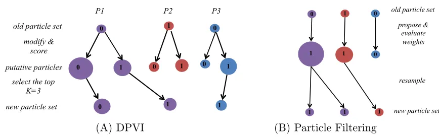
To understand DPVI applied to filtering problems, it is helpful to contemplate three possible fates for a particle at timen (illustrated in Figure 1):
• Selection: A single continuation of particlekhas non-zero weight. This can be seen as a deterministic version of particle filtering, where the sampling operation is replaced with a max operation.
• Splitting: Multiple continuations of particle k have non-zero weight. In this case, the particle is split into multiple particles at the next iteration.
• Deletion: No continuations of particle k have non-zero weight. In this case, the particle is deleted from the particle set.
Similar to particle filtering with resampling, DPVI deletes and propagates particles based on their probability. However, as we show later, DPVI is able to escape some of the problems associated with resampling.
5. Related Work
DPVI is related to several other ideas in the statistics literature:
• DPVI is a special case of a mixture mean-field variational approximation (Jaakkola and Jordan, 1998; Lawrence, 2000):
Q(x) = K X
k=1
Q(k) N Y
n=1
Q(xn|k). (17)
In DPVI, Q(k) =wk and Q(x
n|k) =δ[xn, xkn]. From the simple restriction that the component distributions must be delta functions, we derived a new algorithm that is simpler and more efficient than mixture mean-field (which requires separate updates for the mixture weights), while sacrificing some of its expressivity. Another distinct advantage of DPVI is that the variational updates do not require the additional lower bound used in general mixture mean-field, due to the intractability of the mean-field updates.
0
1 0 1 0 1
0 1 1
0
1 0
modify & score
select the top K=3 old particle set
new particle set putative particles
P1 P2 P3
1 1
1 1 1
1 0 old particle set
new particle set propose &
evaluate weights
resample 0
0
(A) DPVI (B) Particle Filtering
Figure 1: Schematic of DPVI versus particle filtering for filtering problems. Illustration of different filtering scenarios over 2 time steps in a binary state space with
K = 3 particles. The number in each circle indicates the binary value of the corresponding variable. Arrows indicate the evolution of the particles. (A) DPVI: The size of the putative particles represents the score of the particle. The K
continuations with highest score are selected for propagation to the next time step. The size of the new particle set corresponds to the normalized score. Particle
P1 is split, P2 is deleted and one putative particle from P3 is selected. (B) Particle filtering: The size of the node represents the weight of the particle for the resampling step.
such as reconstruction and segmentation of Markov random fields. However, the al-gorithm is susceptible to local optima without the aid of relaxation techniques like simulated annealing (Greig et al., 1989).
• DPVI is conceptually similar to nonparametric variational inference (Gershman et al., 2012), which approximates the posterior over a continuous state space using a set of particles convolved with a Gaussian kernel (see Miller et al., 2016, for more sophisti-cated extensions of this idea). This approach was shown to be effective for probabilis-tic models that lack the conjugate-exponential structure required for exact mean-field inference. Because nonparametric variational inference approximates continuous den-sities, it is inapplicable to the discrete problems considered here.
• Frank et al. (2009) used particle approximations within a variational message passing algorithm. The resulting approximation is “local” in the sense that the particles are used to approximate messages passed between nodes in a factor graph, in contrast to the “global” approximation produced by DPVI, which attempts to capture the distribution over the entire set of variables. It is an interesting question for future research to understand what classes of probabilistic models are better approximated using local vs. global approaches.
truncations as a function of the number of samples. This is similar (though not equivalent) to the DPVI setting where latent variables are sampled exhaustively and without replacement.
• Schniter et al. (2008) described an approximate inference algorithm, fast Bayesian matching pursuit, which can be viewed as a special case of DPVI applied to Gaussian mixture models.
• In Jones et al. (2005), ashotgun stochastic search algorithm is suggested, which pro-poses local changes to the latent variables with probability proportional to the un-normalized posterior. While this method of evaluating local changes is similar to our coordinate algorithm for the DPVI objective, it is important to note that DPVI is not a stochastic search algorithm (unless K= 1): It maintains a collection of particles in order to approximate the posterior distribution, which is important for applications that require a representation of uncertainty.
• Finally, DPVI is closely related to the problem of finding theK most probable latent variable assignments (Flerova et al., 2012; Yanover and Weiss, 2003). We view this problem through the lens of particle approximations, connecting it to both Monte Carlo and variational methods. The techniques developed for finding the K-best assignments could be fruitfully applied to optimizing the DPVI objective function.
Our experimental strategy is to compare DPVI with popular algorithms that have similar computational complexity, which is why we focus on particle filtering, Gibbs sampling and mean-field approximations. Although mixture mean-field will by definition lead to a better approximation, its computational complexity is considerably greater, which may explain why it is has never achieved the popularity of standard mean-field approaches. Some of the approaches listed above are not applicable to the discrete setting (nonparametric variational inference and fast Bayesian matching pursuit), and some are point estimators instead of true probabilistic approximations (iterated conditional modes and shotgun stochastic search).
6. Experiments
(A)
DPVI Monte Carlo Mean-Field
Q(x) =
K X k=1 wk N Y n=1
[xn, xkn] Q(x) = N Y
n=1 Q(xn)
Q(x) = 1
K K X k=1 N Y n=1
[ˆxn,xˆkn]
(B)
State Seq.
[ ] Weight
State Seq.
[ ] Mean-Field Parameters
x0,x1,x2
[0,0,0] [0,1,1] [1,1,1] [1,0,0] [1,0,1] 0.15 0.03 0.32 0.15 0.35 [1,0,1] [1,1,1] [1,1,1] [1,1,1] [1,0,1]
DPVI Monte Carlo Mean-Field
x0,x1,x2
P r(x0= 1, x1= 0, x2= 1|y)⇡0.32
P r(x0= 1, x1= 0, x2= 1|y)⇡0.35 P r(x0= 1, x1= 0, x2= 1|y)⇡0.4
x0 x1 x2
y0 y1 y2
Q(x0= 0) = 0.4
Q(x1= 0) = 0.63
Q(x2= 0) = 0.15
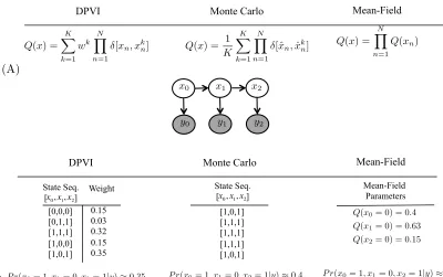
Figure 2: Comparison of approximate inference schemes. (A) Approximating families for DPVI, Monte Carlo and mean-field. (B) Approximating the posterior probability of a sequence (x0= 1, x1 = 0, x2 = 1) for the above 3 schemes on a binary HMM. Given the weights for different sequences in DPVI the posterior probability is the weight corresponding to that sequence. For Monte Carlo approximation, the posterior can be approximated from the normalized counts of sampled (x0 = 1, x1 = 0, x2 = 1) sequences. Finally, for the mean-field approximation, we have
P r(x0 = 1, x1= 0, x2 = 1|y) =Q(x0 = 1)Q(x1= 0)Q(x2= 1).
6.1 Didactic Example: Binary HMM
As a didactic example, we use a simple HMM with binary hidden states (x) and observations (y):
P(xn+1= 0|xn= 0) =α0
P(xn+1= 1|xn= 1) =α1
P(yn= 0|xn= 0) =β0
P(yn= 1|xn= 1) =β1, (18)
0.0001 0.1 1 10 50 Resampling threshold (ESS value)
16 18 20 22 24 26
Total
marginal
error
Particle filter (K=50) DPVI (K=50)
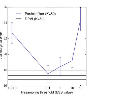
Figure 3: HMM with binary hidden states and observations. Total marginal error computed for a sequence of length 200. For particle filtering the total error for every ESS value is averaged over 5 sequences generated from the HMM; in addition, for each sequence we reran the particle filter 5 times (thus 25 runs total). Note the logarithmic scale of the x-axis. Error bars and the thin black lines correspond to standard error of the mean.
For illustration, we use the following parameters: α0 = 0.2, α1 = 0.1, β0 = 0.3, and
β1 = 0.2. Suppose you observe a sequence generated from this model. For a sufficiently long sequence, a particle filter with resampling will eventually delete most conditionally unlikely particles, due to the fact that there is some probability on each step that any given unlikely particle will be deleted. The particle filter will thus suffer from degeneracy for long sequences. On the other hand, without resampling the approximation will degrade over time because conditionally unlikely particles are never replaced by better particles. For this reason, it is sometimes suggested that resampling only be performed when the effective sample size (ESS) falls below some threshold.
The ESS is calculated as ESS = 1 PK
k=1(wk)2
. A low ESS means that most of the weight is being placed on a small number of particles, and hence the approximation may be degenerate (although in some cases this may mean that the target distribution is peaky). We evaluated particle filtering with multinomial resampling on synthetic data generated from the HMM described above. Approximation accuracy was measured by using the forward-backward algorithm to compute the hidden state posterior marginals exactly and then comparing these marginals to the particle approximation. Figure 3 shows performance as a function of ESS threshold, demonstrating that there is a fairly narrow range of thresholds for which performance is good. Thus in practice, successful applications of particle filtering may require computationally expensive tuning of this threshold.
is automatically tuned to the problem. Instead of resampling particles, DPVI deletes or propagates particles deterministically based on their relative contribution to the variational bound. We can always incrementally add particles, unlike tuning the threshold. So although
K can be viewed as a tuning parameter, we can adapt it with relatively little expense, monotonically increasing the approximation quality in a way that can be easily quantified.
6.2 Dirichlet Process Mixture Model
A DPMM generates data from the following process (Antoniak, 1974; Escobar and West, 1995):
G∼DP(α, G0), θn|G∼G, yn|θn∼F(θn),
whereα≥0 is a concentration parameter andG0 is a base distribution over the parameter
θn of the observation distribution F(yn|θn). Since the Dirichlet process induces clustering of the parameters θintoK distinct values, we can equivalently express this model in terms of a distribution over cluster assignments,xn∈ {1, . . . , C}. The distribution overxis given by the Chinese restaurant process (Aldous, 1985):
P(xn=c|x1:n−1)∝
(
tc ifk≤C+
α ifc=C++ 1,
(19)
wheretcis the number of data points prior tonassigned to clustercandC+is the number of clusters for which tc>0.
6.2.1 Synthetic Data
We first demonstrate our approach on synthetic data sets drawn from various mixtures of bivariate Gaussians (see Table 1). The model parameters for each simulated data set were chosen to create a spectrum of increasingly overlapping clusters. In particular, we constructed models out of the following building blocks:
µ1= 0.0,0.0
, µ2 = 0.5,0.5
Σ1 = 00.25.0,,00..250
, Σ2 = 00..50,,00..05
.
For the DPMM, we used a Normal likelihood with a Normal-Inverse-Gamma prior on the component parameters:
ynd|xn=k∼ N(mkd, σ2kd), mkd∼ N(0, σ2kd/τ), σ2kd ∼IG(a, b), (20) where d∈ {1,2} indexes observation dimensions and IG(a, b) denotes the Inverse Gamma distribution with shape a and scale b. We used the following hyperparameter values: τ = 25, a= 1, b= 1, α= 0.5.
Data set PF (K= 20) MF DPVI (K= 1) DPVI (K= 20) D1: [µ1,4µ2,8µ2],Σ1 0.97±0.03 0.80±0.10 0.93±0.05 0.99±0.02 D2: [µ1,4µ2,8µ2],Σ2 0.89±0.05 0.63±0.02 0.86±0.07 0.90±0.03 D3: [µ1,2µ2,4µ2],Σ1 0.58±0.12 0.53±0.05 0.51±0.03 0.74±0.16 D4: [µ1,2µ2,4µ2],Σ2 0.50±0.06 0.29±0.05 0.46±0.05 0.55±0.07 D5: [µ1, µ2,2µ2],Σ1 0.05±0.05 0.28±0.12 0.014±0.02 0.14±0.10 D6: [µ1, µ2,2µ2],Σ2 0.15±0.08 0.12±0.03 0.11±0.06 0.19±0.07 Table 1: Clustering accuracy (V-Measure) for DPMM. Each data set consisted of 200 points
drawn from a mixture of 3 Gaussians. For each data set, we repeated the experi-ment 150 times by iterating through random seeds, reporting mean and standard error. The left column shows the ground truth mean for each cluster and the covariance matrix (shared across clusters). PF denotes particle filtering and MF denotes mean-field.
Number of particles DPVI Particle Filtering
K = 10 15.20s 14.71s
K = 50 153.75s 184.17s
K = 100 567.84s 699.43s
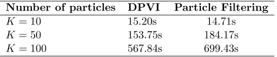
Table 2: Run time comparison for DPMM with synthetic data using data set from Table 1. The run time of DPVI is slightly better than particle filtering for a single pass through the data set.
shown in Table 1, we observe only marginal improvements when the means are farthest from each other and variances are small, as these parameters leads to well-separated clusters in the training set. However, the relative accuracy of DPVI increases considerably when the clusters are overlapping, either due to the fact that the means are close to each other or the variances are high. One factor contributing to greater performance of DPVI might be the diversity term in the variational formulation.
An interesting special case is whenK= 1. In this case, DPVI is equivalent to the greedy algorithm proposed by Daume (2007) and later extended by Wang and Dunson (2011). In fact, this algorithm was independently proposed in cognitive psychology by Anderson (1991). As shown in Table 1, DPVI with 20 particles outperforms the greedy algorithm, as well as particle filtering with 20 particles. We also demonstrate the run-time performance of DPVI compared to particle filtering in Table 2. It can be seen in our experiments that DPVI tends to be comparable to particle filtering or sometimes more efficient in terms of run-time for the same task, although the theoretical complexity is the same.
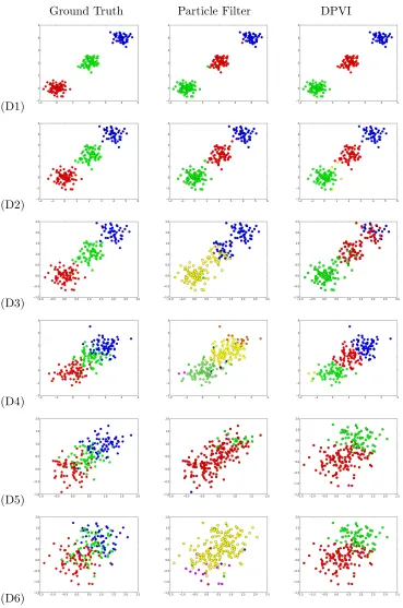
6.2.2 Spike Sorting
Ground Truth Particle Filter DPVI
(D1)
(D2)
(D3)
(D4)
(D5)
(D6)
The goal is to extract from noisy spike recordings attributes such as the number of neurons, and cluster spikes belonging to the same neuron. This problem naturally motivates the use of DPMM, since the number of neurons recorded by a single tetrode is unknown. Previ-ously, Wood and Black (2008) applied the DPMM to spike sorting using particle filtering and Gibbs sampling. Here we show that DPVI can outperform particle filtering, achieving high accuracy even with a small number of particles.
We used data collected from a multiunit recording from a human epileptic patient (Quiroga et al., 2004). The raw spike recordings were preprocessed following the proce-dure proposed by Quiroga et al. (2004), though we note that our inference algorithm is agnostic to the choice of preprocessing. The original data consist of an input vector with
D = 10 dimensions and 9196 data points. Following Wood and Black (2008), we used a Normal likelihood with a Normal-Inverse-Wishart prior on the component parameters:
yn|xn=k∼ N(mk,Λk), mk∼ N(0,Λk/τ), Λk∼IW(Λ0, ν), (21) where IW(Λ0, ν) denotes the Inverse Wishart distribution with degrees of freedom ν and scale matrix Λ0. We used the following hyperparameter values: ν = D+ 1,Λ0 = I, τ = 0.01, α= 0.1.
We compared our algorithm to the current best particle filtering baseline, which uses stratified resampling (Wood and Black, 2008; Fearnhead, 2004). The same model param-eters were used for all comparisons. Qualitative results, shown in Figure 5B, demonstrate that DPVI is better able to separate the spike waveforms into distinct clusters, despite running DPVI with 10 particles and particle filtering with 100 particles. We also provide quantitative results by calculating the held-out log-likelihood on an independent test set of spike waveforms. The quantitative results (summarized in Table 5C) demonstrate that even with only 10 particles DPVI can outperform particle filtering with 1000 particles.
6.3 Infinite HMM
An iHMM generates data from the following process (Teh et al., 2006):
G0 ∼DP(γ, H), Gk|G0∼DP(α, G0),
xn|xn−1 ∼Gxn−1, θk ∼H, yn|xn∼F(θxn).
Like the DPMM, the iHMM induces a sequence of cluster assignments. The distribution over cluster assignments is given by the Chinese restaurant franchise (Teh et al., 2006). Letting tjc denote the number of times cluster j transitioned to cluster c, xn is assigned to cluster c with probability proportional totxn−1c, or to a cluster never visited from xn−1 (txn−1c = 0) with probability proportional to α. If an unvisited cluster is selected, xn is assigned to cluster c with probability proportional toPjtjc, or to a new cluster (i.e., one never visited from any state,Pjtjc= 0) with probability proportional to γ.
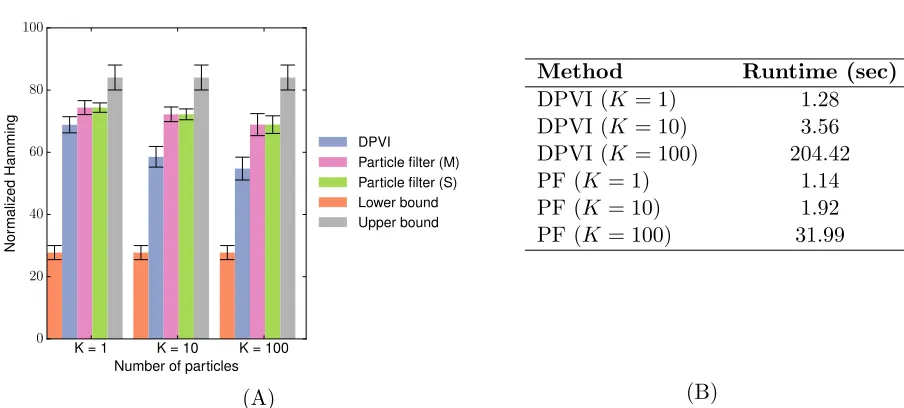
6.3.1 Synthetic Data
(A)
(B)
Method Predictive LL
DPVI (K= 10) -3.2474×10⁵ ( ˆC = 3) DPVI (K= 100) -1.3888×10⁵ (Cˆ =3) PF (K= 10) -1.4771±0.21×10⁶ ( ˆC= 37) PF (K= 100) -5.6757±1.14×10⁵ ( ˆC= 13) PF (K= 1000) -3.2965×10⁵ ( ˆC = 5)
(C)
Method Run time
DPVI (K= 10) 36.20s
DPVI (K= 50) 144.6s
DPVI (K= 100) 313.8s
PF (K= 10) 124s
PF (K= 50) 334.2s
PF (K= 100) 454.2s
(D)
K = 1 K = 10 K = 100 Number of particles
0 20 40 60 80 100
Nor
maliz
ed
Hamming
DPVI
Particle filter (M) Particle filter (S) Lower bound Upper bound
(A)
Method Runtime (sec)
DPVI (K = 1) 1.28
DPVI (K = 10) 3.56
DPVI (K = 100) 204.42
PF (K = 1) 1.14
PF (K = 10) 1.92
PF (K = 100) 31.99
(B)
HMMs we used a symmetric Dirichlet prior with concentration parameter 0.1; for the emis-sion probability matrix, we used a symmetric Dirichlet prior with concentration parameter 10.
Figure 6A illustrates the performance of DPVI and particle filtering (with multinomial and stratified resampling) for varying numbers of particles (K = 1,10,100). Performance error was quantified by computing the Hamming distance between the true hidden sequence and the sampled sequence. The Munkres algorithm was used to maximize the overlap between the two sequences. The results show that DPVI outperforms particle filtering in all three cases.
When the data consist of long sequences, resampling at every step will produce degen-eracy in particle filtering; this tends to result in a smaller number of clusters relative to DPVI. The superior accuracy of DPVI suggests that a larger number of clusters is necessary to capture the latent structure of the data. Not surprisingly, this leads to longer run times (Figurets 6B), but it is important to note that particle filtering and DPVI have comparable per-cluster time complexity.
1 10 50 100
Number of particles
−1.20
−1.15
−1.10
−1.05
−1.00
−0.95
Predictiv
e
log-lik
elihood
×104
DPVI Particle filter Beam sampler
(A)
Method Runtime (sec)
DPVI (K = 1) 4.73
DPVI (K = 10) 41.62
DPVI (K = 100) 1685
PF (K = 1) 1.64
PF (K = 10) 28.08
PF (K = 100) 211.66
Beam sampler 260
(B)
Figure 7: Infinite HMM for the text analysis task. (A) Predictive log-likelihood for the Alice in Wonderland data set. (B) Results using the “Alice in Wonderland” data set. The maximum number of inferred clusters is ˆC = 147 for DPVI (K = 100) and ˆC= 21 for particle filter (K = 100). As expected, the per cluster runtime of the two methods are comparable.
6.3.2 Text Analysis
and the subsequent 4000 characters for test. Performance was measured by calculating the predictive log-likelihood. We fixed the hyperparameters α and γ to 1 for both DPVI and the particle filtering.
We ran one pass of DPVI (filtering) and particle filtering over the training sequence. We then sampled 50 data sets from the distribution over the sequences. We truncated the number of states and used the learned transition and emission matrices to compute the predictive log-likelihood of the test sequence. To handle the unobserved emissions in the test sequence we used “add-δ” smoothing with δ = 1. Finally, we averaged over all the 50 data sets.
We also compared DPVI to the beam sampler (Van Gael et al., 2008), a combination of dynamic programming and slice sampling, which was previously applied to this data set. For the beam sampler, we followed the setting of Van Gael et al. (2008). We run the sampler for 10000 iterations and collect a sample of hidden state sequence every 200 iterations. Figure 6B shows the predictive log-likelihood for varying numbers of particles. Even with a small number of particles, DPVI can outperform both particle filtering and the beam sampler.
6.3.3 User Behavior Analysis
We analyzed a data set of user behavior in a photo editing software application. The data set contains sequences of edits applied by users to different photos. An iHMM can be utilized for better understanding the high-level tasks of the users. That is, a sequence of multiple edits may be required to perform a high-level task such as cropping or masking a photo. Our data set contains 30000 edits from which we use 1000 data points as a held-out set. There are 23 possible observations (edits) in the data set. We compare DPVI with 1, 5 and 10 particles with particle filtering, Gibbs sampling and mean field inference schemes. For all the inference schemes, we set the hyperparametersαandγ to 1. In every iteration of DPVI and particle filtering, we do a forward filtering-backward smoothing pass over all the sequences of the data set. Our results, shown in Figure 8(B), demonstrate that DPVI with 5 and 10 particles can converge in fewer iterations compared to other reasonable baselines. We illustrate the lower bound (Eq. 10) convergence in Figure 9. The results are computed over 20 runs and for 1, 5 and 10 particles.
It is important to note here that we do not expect DPVI to outperform Gibbs sampling in all scenarios; when computation time is not strongly limited, we expect DPVI and Gibbs to perform similarly. This point applies here as well as to the experiments reported in the sections below. We see DPVI as a useful alternative to Gibbs when the computational budget is low and the required fidelity of the approximation can be satisfied by capturing a few of the posterior modes.
6.4 Infinite Relational Model (IRM)
0 500 1000 1500 2000 2500 3000 Iteration
−3400
−3200
−3000
−2800
−2600
−2400
−2200
−2000
−1800
Predictiv
e
log-lik
elihood
DPVI 1 DPVI 5 DPVI 10
PF 1 PF 5 PF 10
Gibbs MF
(A)
Method Predictive LL
DPVI (K= 1) −2983.24±93.77 DPVI (K= 5) −2018.02±9.23 DPVI (K= 10) −2058.75±33.62 PF (K= 1) −2743.60±28.49 PF (K= 5) −2503.95±40.46 PF (K= 10) −2424.01±72.72 Mean field −3158.69±52.67 Gibbs −2030.50±56.55
(B)
0 500 1000 1500 2000 2500 3000 Iteration
−2.6
−2.4
−2.2
−2.0
−1.8
−1.6
−1.4
L
[
Q
]
×104
DPVI 1 DPVI 5 DPVI 10
Figure 9: Infinite HMM results for the user behavior analysis task. Lower bound vs iteration for the user behavior data set. The error bars correspond to the standard error and are computed over 20 runs. In every iteration of DPVI, we do a forward filtering-backward smoothing pass over all the sequences of the data set.
Given a relation R involving J types of entities, the goal is to infer a vector of cluster assignments xj for all the entities of each type j = 1, . . . , J.2 Assuming the cluster as-signments for each type are independent, the joint density of the relation and the cluster assignment vectors can be written as:
P(R, x1, . . . , xJ) =P(R|x1, . . . , xJ) J Y
j=1
P(xj). (22)
The cluster assignment vectors are drawn from a CRP(α) prior. Given the cluster assign-ment vectors, the relations are drawn from a Bernoulli distribution with a parameter η
that depends on the clusters involved in that relation. For instance, in a single two-place relation, η(a, b) is the probability of having a link between any given pair (i, j) where i is in cluster aand j is in clusterb.
More formally, let us define an M dimensional relationR:Td1×. . . TdM 7→ {0,1}, over J different types. Each relational value is generated according to:
R(i1, . . . , iM)|x1, . . . , xJ ∼Bernoulli(η(xdi11, . . . , x
dM
iM )), (23)
wheredmdenotes the label of the type (i.e.,dm ∈ {1,· · ·, J}) andim is the entity occupying position m in the relation. Each entry of parameter matrix η is drawn from a Beta(β, β) distribution. By using a conjugate Beta-Bernoulli model, we can analytically marginalize the parameters η (see Kemp et al., 2006), allowing us to directly compute the likelihood of the relational matrix given the cluster assignments,P(R|x1, . . . , xJ).
We compared the performance of DPVI with Gibbs sampling, using predictive log-likelihood on held-out data as a performance metric. The “animals” data set analyzed in
Sample animal clusters:
A1: Hippopotamus, Elephant, Rhinoceros A2: Seal, Walrus, Dolphins, Blue Whale,
Killer Whale, Humpback Whale A3: Beaver, Otter, Polar Bear
Sample feature clusters: F1: Hooves, Long neck, Horns
F2: Inactive, Slow, Bulbous Body, Tough Skin F3: Lives in Fields, Lives in Plains, Grazer F4: Walks, Quadrupedal, Ground
F5: Fast, Agility, Active, Tail
Figure 10: Co-clustering of animals (rows) and features (columns) after 50 iterations of DPVI with 10 particles in the infinite relational model.
Kemp et al. (2006), was used for this task. This data set (Osherson et al., 1991) is a two type data set R : T1 ×T2 → {0,1} with animals and features as it types; it contains 50 animals and 85 features.
We removed 20% of the relations from the data set and computed the predictive log-likelihood for the held-out data. We ran DPVI with 1, 10 and 20 particles for 1000 iterations. Given the weights of the particles, we computed the weighted log-likelihood. We also ran 20 independent runs of the Gibbs sampler and DPVI for 1000 iterations and computed the average predictive log-likelihood. Every iteration scans all the data points in all the types sequentially. We set the hyperparameters α and β to 1. Figure 10 illustrates the co-clustering discovered by DPVI for the data set, demonstrating intuitively reasonable animal and feature clusters.
The results after 1000 iterations are presented in Table 11B. The best performance is achieved by DPVI with 20 particles. Figure 11A shows the predictive log-likelihood for every iteration of DPVI and Gibbs sampling. DPVI with 10 and 20 particles converge in 11 and 18 iterations, respectively. In terms of computation time per iteration of DPVI versus Gibbs, the only difference for DPVI with one particle and Gibbs is the sorting cost. Hence, for the multiple particle versus multiple runs of Gibbs sampling, the only additional cost is the sorting cost for multiple particles (e.g. 10 or 20). However, this insignificant additional cost is compensated for by a faster convergence rate in our experiments.
6.5 Ising Model
So far, we have been studying inference in directed graphical models, but DPVI can also be applied to undirected graphical models. We illustrate this using the Ising model for binary vectors x∈ {−1,+1}N:
f(x) = exp
1 2xW x
>+θx>
0 200 400 600 800 1000 Iteration
−480
−460
−440
−420
−400
−380
−360
Predictiv
e
log-lik
elihood
DPVI 1 DPVI 10 DPVI 20 Gibbs
(A)
Method Predictive LL
DPVI (K= 1) −418.49±4.24 DPVI (K= 10) −382.46±7.34 DPVI (K= 20) −370.67±6.23 Gibbs (avg. of 20 runs) −371.74±5.07
(B)
Figure 11: Infinite relational model results for the animals data set. (A) Predictive log-likelihood vs iteration for the animals data set. The error bars correspond to the standard error and for both methods are computed over 20 runs. (B) Pre-dictive log-likelihood after 1000 iterations of DPVI and Gibbs (with 50 burnin iterations) for the animals data set (with 20 % held-out). DPVI with 20 particles performs in par with the Gibbs sampler.
where W ∈ RN×N and θ ∈ RN are fixed parameters. In particular, we study a square
lattice ferromagnet, where Wij =β for neighboring nodes (0 otherwise) and θi = 0 for all nodes. We refer to β as the coupling strength. This model has two global modes: when all the nodes are set to 1, and when all the nodes are set to 0. As the coupling strength increases, the probability mass becomes increasingly concentrated at the two modes.
We applied DPVI to this model, varying the number of particles and the coupling strength. At each iteration, we evaluated the change in log probability that would result from setting ˜xk
n= 1:
akn= X n0∈c n
Wn,n0xkn0+θn, (25)
and likewise the change for setting ˜xk
n= 1 can be computing by simply flipping the sign of ak
1 2 3 4 60.6
60.8 61 61.2 61.4 61.6 61.8 62
Coupling strength: 0.01
Number of particles
log Z
Q
− log Z
MF
1 2 3 4
1400.2 1400.3 1400.4 1400.5 1400.6 1400.7 1400.8 1400.9 1401
Coupling strength: 100
Number of particles
log Z
Q
− log Z
MF
Figure 12: Ising model results. Difference between DPVI and mean-field lower bounds on the partition function. Positive values indicates superior DPVI performance. (A) Low coupling strength; (B) high coupling strength.
To illustrate the performance of DPVI further, we compared several posterior approxi-mations for the Ising model in Figure 13. In addition to the mean-field approximation, we also compared DPVI with two other standard approximations: the Swendsen-Wang Monte Carlo sampler (Swendsen and Wang, 1987) and loopy belief propagation (Murphy et al., 1999). The sampler tended to produce noisy results, whereas mean-field and BP both failed to capture the multimodal structure of the posterior. In contrast, DPVI with two particles perfectly captured the two modes.
7. Conclusions
This paper introduced a particle-based variational method that applies to a broad class of inference problems in discrete models. We described a practical algorithm for optimizing the particle approximation, and showed empirically that it can outperform widely-used Monte Carlo and variational algorithms. The key to the success of this approach is an intentional selection of particles: rather than generating them randomly (as in Monte Carlo algorithms), we deterministically choose a set of unique particles that optimizes the KL divergence between the approximation and the target distribution.
This approach leads to an interesting view on the problem of resampling in sequential Monte Carlo. Resampling is necessary to remove conditionally unlikely particles, but the resulting loss of particle diversity can lead to degeneracy. As we showed in our experiments, tuning an ESS threshold for resampling can improve performance, but requires finding a relatively narrow sweet spot for the threshold. DPVI achieves comparable performance to the best particle filter by using a deterministic strategy for deleting and replacing particles and does not require tuning thresholds. Each particle is guaranteed to be unique and have high probability among all states discovered so far.
Samples
Samples
DPVI
DPVI
Mean field
BP
Figure 13: Ising model simulations. Examples of posteriors for the ferromagnetic lattice at low coupling strength. (Top) Two configurations from a Swendsen-Wang sampler. (Middle) Two DPVI particles. (Bottom left) Mean-field expected value. (Bottom right) Loopy belief propagation expected value.
we may need to know the output probability density of the particle extension mechanism. However, if we use the results in DPVI, we just need to be able to score the results under the joint probability distribution. No proposal distribution is needed. This could make it possible to use proposal mechanisms that can be seen to work well empirically but that are difficult to analyze a priori.
Although our empirical results are promising, much more empirical and theoretical work is needed to understand the fundamental tradeoffs between variational and Monte Carlo inference. However, the results for DPVI on several problems are promising, and the approach to defining variational approximations may be more broadly applicable. We hope this work encourages others to develop different hybrids of Monte Carlo and variational inference that overcome the limitations of each approach when used in isolation.
Acknowledgments
TDK was generously supported by the Leventhal Fellowship. VKM is supported by the
Army Research Office Contract Number 0010363131, Office of Naval Research Award N000141310333, and the DARPA PPAML program. The views and conclusions contained herein are those of
authorized to reproduce and distribute reprints for Governmental purposes notwithstanding any copyright annotation thereon.
References
David Aldous. Exchangeability and related topics. Ecole d’ ´´ Et´e de Probabilit´es de Saint-Flour XIII1983, pages 1–198, 1985.
John R Anderson. The adaptive nature of human categorization. Psychological Review, 98: 409–429, 1991.
Charles E Antoniak. Mixtures of Dirichlet processes with applications to Bayesian non-parametric problems. The Annals of Statistics, pages 1152–1174, 1974.
Matthew J Beal, Zoubin Ghahramani, and Carl E Rasmussen. The infinite hidden Markov model. In Advances in Neural Information Processing Systems, pages 577–584, 2002.
Julian Besag. On the statistical analysis of dirty pictures. Journal of the Royal Statistical Society. Series B (Methodological), 48:259–302, 1986.
Alexandre Bouchard-Cˆot´e and Michael I Jordan. Optimization of structured mean field objectives. In Proceedings of the Twenty-Fifth Conference on Uncertainty in Artificial Intelligence, pages 67–74. AUAI Press, 2009.
Hal Daume. Fast search for Dirichlet process mixture models. InInternational Conference on Artificial Intelligence and Statistics, pages 83–90, 2007.
Arnaud Doucet, Nando De Freitas, Neil Gordon, et al. Sequential Monte Carlo Methods in Practice. Springer New York, 2001.
Michael D Escobar and Mike West. Bayesian density estimation and inference using mix-tures. Journal of the American Statistical Association, 90:577–588, 1995.
Paul Fearnhead. Particle filters for mixture models with an unknown number of components.
Statistics and Computing, 14:11–21, 2004.
Natalia Flerova, Emma Rollon, and Rina Dechter. Bucket and mini-bucket schemes for m best solutions over graphical models. In Graph Structures for Knowledge Representation and Reasoning, pages 91–118. Springer, 2012.
Andrew Frank, Padhraic Smyth, and Alexander T Ihler. Particle-based variational inference for continuous systems. In Advances in Neural Information Processing Systems, 2009.
Samuel Gershman, Matt Hoffman, and David Blei. Nonparametric variational inference.
Proceedings of the 29th International Conference on Machine Learning, 2012.
Peter Hall, John T Ormerod, and MP Wand. Theory of Gaussian variational approximation for a Poisson mixed model. Statistica Sinica, 21:369–389, 2011.
Edward L Ionides. Truncated importance sampling. Journal of Computational and Graph-ical Statistics, 17:295–311, 2008.
Tommi S Jaakkola and Michael I Jordan. Improving the mean field approximation via the use of mixture distributions. In MI Jordan, editor, Learning in Graphical Models, pages 163–173. Springer, 1998.
Beatrix Jones, Carlos Carvalho, Adrian Dobra, Chris Hans, Chris Carter, and Mike West. Experiments in stochastic computation for high-dimensional graphical models. Statistical Science, 20:388–400, 2005.
Charles Kemp, Joshua B Tenenbaum, Thomas L Griffiths, Takeshi Yamada, and Naonori Ueda. Learning systems of concepts with an infinite relational model. InAAAI, volume 3, page 5, 2006.
Neil D Lawrence. Variational inference in probabilistic models. PhD thesis, University of Cambridge, 2000.
Kerrie L Mengersen, Richard L Tweedie, et al. Rates of convergence of the Hastings and Metropolis algorithms. The Annals of Statistics, 24:101–121, 1996.
Sean P Meyn and Richard L Tweedie. Markov Chains and Stochastic Stability. Springer-Verlag, 1993.
Andrew C Miller, Nicholas Foti, and Ryan P Adams. Variational boosting: Iteratively refining posterior approximations. arXiv preprint arXiv:1611.06585, 2016.
Kevin P Murphy, Yair Weiss, and Michael I Jordan. Loopy belief propagation for ap-proximate inference: An empirical study. In Proceedings of the Fifteenth conference on Uncertainty in artificial intelligence, pages 467–475. Morgan Kaufmann Publishers Inc., 1999.
Daniel N Osherson, Joshua Stern, Ormond Wilkie, Michael Stob, and Edward E Smith. Default probability. Cognitive Science, 15:251–269, 1991.
Rodrigo Quian Quiroga, Zoltan Nadasdy, and Yoram Ben-Shaul. Unsupervised spike detec-tion and sorting with wavelets and superparamagnetic clustering. Neural computation, 16:1661–1687, 2004.
Christian P Robert and George Casella. Monte Carlo Statistical Methods. Springer, 2004.
Andrew Rosenberg and Julia Hirschberg. V-measure: A conditional entropy-based external cluster evaluation measure. InEMNLP-CoNLL, volume 7, pages 410–420, 2007.
Philip Schniter, Lee C Potter, and Justin Ziniel. Fast Bayesian matching pursuit. In
Robert H Swendsen and Jian-Sheng Wang. Nonuniversal critical dynamics in Monte Carlo simulations. Physical Review Letters, 58:86–88, 1987.
Yee Whye Teh, Michael I Jordan, Matthew J Beal, and David M Blei. Hierarchical Dirichlet processes. Journal of the American Statistical Association, 101:1566–1581, 2006.
Jurgen Van Gael, Yunus Saatci, Yee Whye Teh, and Zoubin Ghahramani. Beam sampling for the infinite hidden Markov model. InProceedings of the 25th international conference on Machine learning, pages 1088–1095. ACM, 2008.
Martin J Wainwright and Michael I Jordan. Graphical models, exponential families, and variational inference. Foundations and Trends in Machine Learning, 1:1–305, 2008.
Bo Wang, DM Titterington, et al. Convergence properties of a general algorithm for calcu-lating variational bayesian estimates for a normal mixture model. Bayesian Analysis, 1: 625–650, 2006.
Lianming Wang and David B Dunson. Fast Bayesian inference in Dirichlet process mixture models. Journal of Computational and Graphical Statistics, 20, 2011.
Frank Wood and Michael J Black. A nonparametric Bayesian alternative to spike sorting.
Journal of Neuroscience Methods, 173:1–12, 2008.