772
Copyright © 2011-15. Vandana Publications. All Rights Reserved.
Volume-5, Issue-2, April-2015
International Journal of Engineering and Management Research
Page Number: 772-779
Evaluation of Material Removal Rate and Surface Roughness in Turning
Using Response Surface Methodology
B. Naga Raju1, M.Raja Roy2, A.Rohit3
1
Associate Professor, Department of Mechanical Engineering, ANITS, Visakhapatnam, Andhra Pradesh, INDIA
2
Sr. Assistant Professor, Department of Mechanical Engineering, ANITS, Visakhapatnam, Andhra Pradesh, INDIA
3
Department of Mechanical Engineering, ANITS, Visakhapatnam, Andhra Pradesh, INDIA
ABSTRACT
The Quality and productivity plays a significant role in today’s manufacturing market. Therefore, every manufacturing or production unit concerns about the quality of the product. Apart from quality, there exists another criterion, called productivity which is directly related to the profit level and also goodwill of the organization. This invites optimization technique which seeks identification of the best process condition or parametric combination for the said manufacturing process. In order to tackle multi-objective optimization problems, the authors have made an attempt to present Full Factorial Method in straight turning of Mild Steel bar using HSS tool. Experiments were conducted in a series of tests called runs, in which changes are made in the input variables in order to identify the reasons for changes in the output response using Response Surface Methodology (RSM). The predicted optimal setting ensured the minimization of Surface Roughness and maximization of Material Removal Rate (MRR).
Keywords—Material Removal Rate, Surface Roughness,
Design of Experiments, Response Surface Methodology
I.
INTRODUCTION
1.1 Lathe Machine
Lathe removes undesired material from a rotating work piece in the form of chips with the help of tool which is traversed across the work and can be fed deep into the work. The tool material should be harder than the work piece and latter held securely and rigidly on the machine as shown in the Fig: 1.1. The tool may be given linear motion in any direction.
Tool
Support Support
Job
Fig: 1.1
1.2 Cutting Parameters in Turning
The three primary factors in any basic turning operation are speed, feed, and depth of cut. Other factors such as kind of material and type of tool have a large influence, of course, but these three are the ones the operator can change by adjusting the controls, right at the machine.
1.2.1 Speed
Speed always refers to the spindle and the work piece. When it is stated in revolutions per minute (rpm) it tells their rotating speed. But the important feature for a particular turning operation is the speed at which the work piece material is moving past the cutting tool. It is simply the product of the rotating speed times the circumference of the work piece before the cut is started. It is expressed in meter per minute (m/min), and it refers only to the work piece. Every different diameter on a work piece will have a different cutting speed, even though the rotating speed remains the same.
V = π DN/1000 m/min
Here, Vis the cutting speed
773
Copyright © 2011-15. Vandana Publications. All Rights Reserved.
and N is the spindle speed in RPM. 1.2.2 Feed
Feed always refers to the cutting tool, and it is the rate at which the tool advances along its cutting path. On most power-fed lathes, the feed rate is directly related to the spindle speed and is expressed in mm (of tool advance) per r evolution (of the spindle), mm/rev.
Fm = f N mm /min
Here, Fm is the feed in mm per minute,
f is the feed in mm/rev and N is the spindle speed in RPM.
1.2.3 Depth of Cut
Depth of cut is practically self explanatory. It is the thickness of the layer being removed (in a single pass) from the work piece or the distance from the uncut surface of the work to the cut surface, expressed in mm. It is important to note, though, that the diameter of the work piece is reduced by two times the depth of cut because this layer is being removed from both sides of the work.
Dcut= (D – d) /2 mm
Here, Dcut represents the depth of cut
D and d represent initial and final diameter (in mm) of the job respectively.
1.3 Metal Removal Rate
The Material Removal Rate (MRR) in turning operations is the volume of material/metal that is removed per unit time in mm3/min. For each revolution of the work piece, a ring shaped layer of material is removed as shown in Fig:1.2.
Fig: 1.2 Metal Removal Rate
1.4 Surface Roughness
Surface roughness is an important measure of product quality since it greatly influences the performance of mechanical parts as well as production cost. Surface roughness has an impact on the mechanical properties like fatigue behaviour, corrosion resistance, creep life, etc. It also affects other functional attributes of parts like friction, wear, light reflection, heat transmission, lubrication, electrical conductivity, etc. Before surface roughness, it is
also necessary to discuss about surface structure and properties, as they are closely related.
Upon close examination of the surface of a piece of metal, it can be found that it generally consists of several layers as shown in Fig: 1.3. The characteristics of these layers are briefly outlined here:
Fig: 1.3: Schematic representation of cross-section of the surface structure of metals
1.5 Mild Steel
Mild Steel is a type of steel that only contains a small amount of carbon and other elements. It is softer and more easily shaped than higher carbon steels. It also bends a long way instead of breaking because it is ductile. It is used in nails and some types of wire, it can be used to make bottle openers, chairs, staplers, staples, railings and most common metal products. Its name comes from the fact it only has less carbon than steel.
Some mild steel properties and uses:
• Mild Steel has a maximum limit of 0.2% carbon. The proportions of manganese (1.65%), copper (0.6%) and silicon (0.6%) are approximately fixed, while the proportions of cobalt, chromium, niobium, molybdenum, titanium, nickel, tungsten, vanadium and zirconium are not.
• A higher amount of carbon makes steels different from low carbon mild-type steels. A greater amount of carbon makes steel stronger, harder and very slightly stiffer than a low carbon steel. However, the strength and hardness comes at the price of a decrease in the ductility of this alloy. Carbon atoms get trapped in the interstitial sites of the iron lattice and make it stronger.
1.6 High speed steels (HSS)
HSS tools are so named because they were developed to cut at higher speeds. Developed around 1900 HSS are the most highly alloyed tool steels. The tungsten (T series) was developed first and typically contains 12 - 18% tungsten, plus about 4% chromium and 17- 5% vanadium. Most grades contain about 0.5% molybdenum and most grades contain 4 - 12% cobalt.
II.
LITERATURE REVIEW
774
Copyright © 2011-15. Vandana Publications. All Rights Reserved.
Life On Conventional Dry Turning. The surface quality and metal removal rate of the work piece were analyzed and the potential effects of variables such as cutting speed, feed and depth of cut with two different work pieces aluminium alloy and resin on these dependent variables were investigated.
Naga Phani Sastry et al [2] investigated about the “ Analysis and Optimization of Machining Process Parameters using Design of Experiments”. They reported that the surface roughness and MRR parameters greatly depend on work piece materials. A response surface optimization is attempted using DESIGN EXPERT software for output responses in turning. The same idea is implemented in this project by implementation of Minitab software for design of experiments.
Suresh Babu et al [3] presented a paper on “Optimization of cutting parameters for CNC turned parts
using Taguchi’s technique”. Experimentation was
conducted using Taguchi’s technique with an aluminium shaft on a CNC lathe with cutting speed, feed rate and depth of cut as process parameters. The data were analyzed and appropriate process parameters were selected for minimum energy consumption.
Ganesan [4] studied on “Optimization of Machining Parameters in Turning Process Using Genetic Algorithm and Particle Swarm Optimization with Experimental Verification”. He reported that the optimal machining parameters for continuous profile machining are determined with respect to the minimum production time, subject to a set of practical constraints, cutting force, power dimensional accuracy and surface finish. Due to complexity of this machining optimization problem, a genetic algorithm (GA) and Particle Swarm Optimization (PSO) are applied to resolve the problem.
Buragohain [5] presented a paper on “Full Factorial Method” which is used in the design of experiments. Nuran Bradley [6] presented a paper on “Response Surface Methodology” which is used in the optimization of properties of a metal.
III. EXPERIMENTATION
3.1 Design of Experiments
Design of Experiments is an experimental or analytical method that is commonly used to statistically signify the relationship between input parameters to output responses. DOE has wide applications especially in the field of science and engineering for the purpose of process optimization and development, process management and validation tests. DOE is essentially an experimental based modeling and is a designed experimental approach which is far superior to unplanned approach whereby a systematic way will be used to plan the experiment, collect the data and analyze the data. A mathematical model has been developed by Response Surface Methodology.
Optimization and Desirability functions helps to optimize the quality characteristics considered in a DOE under a cost effective process.
3.2 Process Variables
The Process variables and their limits along with code values which are used for conducting the experimentation on mild steel specimens are reported in Table3.1.
3.3 Minitab Software
Minitab is a statistics package. It was developed at the Pennsylvania State University by researchers Barbara F. Ryan, Thomas A. Ryan, Jr., and Brian L. Joiner in 1972. Minitab began as a light version of MNITAB, a statistical analysis program by NIST. Minitab is distributed by Minitab Inc, a privately owned company headquartered in State College. Pennsylvania, with subsidiaries in Coventry, England, Paris, France and Sydney, Australia Today, Minitab is often used in conjunction with the implementation of Six sigma, CMMI and other statistics-based process improvement methods.
3.4 Full Factorial Method
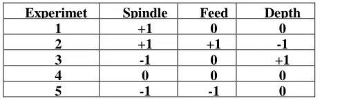
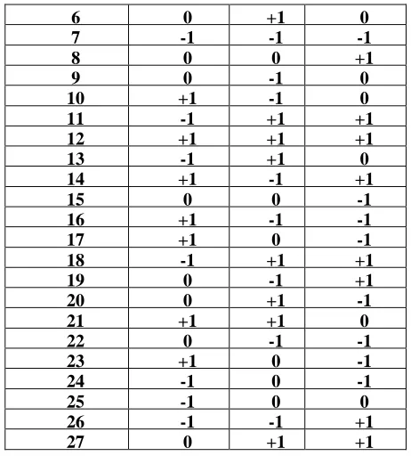
Experiments have been carried out using full factorial method. Experimental design which consists of 27 combinations of spindle speed, longitudinal feed rate and depth of cut. According to the design catalogue prepared by factorial design of experiment has been found suitable in the present work. It considers three process parameters (without interaction) to be varied in three discrete levels. The experimental design has been shown in Table 3.2 (all factors are in coded form). Factorial design is used for conducting experiments as it allows study of interactions between factors. Interactions are the driving force in many processes.
Table 3.2 DOE in Coded form
Experimet Spindle Feed Depth
1 +1 0 0
2 +1 +1 -1
3 -1 0 +1
4 0 0 0
775
Copyright © 2011-15. Vandana Publications. All Rights Reserved.
6 0 +1 0
7 -1 -1 -1
8 0 0 +1
9 0 -1 0
10 +1 -1 0
11 -1 +1 +1
12 +1 +1 +1
13 -1 +1 0
14 +1 -1 +1
15 0 0 -1
16 +1 -1 -1
17 +1 0 -1
18 -1 +1 +1
19 0 -1 +1
20 0 +1 -1
21 +1 +1 0
22 0 -1 -1
23 +1 0 -1
24 -1 0 -1
25 -1 0 0
26 -1 -1 +1
27 0 +1 +1
3.5 Calculation of Material Removal Rate
Material Removal Rate (MRR) has been calculated from the difference of weight of work piece before and after experiment. MS bars of diameter 25.4mm and length 40mm each is required for conducting the experiment has been prepared first. Twenty seven number of samples of same material and same dimensions have been made. After that, the weight of each samples have been measured accurately with the help of a high precision digital balance meter. Metal removal rate is calculated experimentally for each piece using the formula
MRR= ( Wi-Wf ) /Rs*t
Where, Wi & Wf are initial and final weights of the work piece respectively.
Rs is the density of the mild steel work piece (7.8 x10
-3
g/mm3).
t is the time taken for machining
The weight of the work piece has been measured in a high precision digital balance meter (Model: DHD – 200 Macro single pan DIGITAL reading electrically operated analytical balance made by Dhona Instruments), which can measure up to the accuracy of 10-4 g and thus eliminates the possibility of large error while calculating Material Removal Rate (MRR) in straight turning operation.
3.6 Surface Roughness
Surface Roughness is measured using Surface Roughness Tester which directly shows the reading when placed on the metal surface. It consists of a stylus which moves on to the surface of the metal, on pressing the power button. This directly shows the surface value in terms of any desired units. Fig 3.1 shows the surface roughness tester.
Fig 3.1 Surface Roughness Tester.
IV.
RESUTS AND DISCUSSIONS
4.1 Response Surface Methodology
Response surface methodology uses statistical models, and therefore practitioners need to be aware that even the best statistical model is an approximation to reality. In practice, both the models and the parameter values are unknown, and subject to uncertainty on top of ignorance. Of course, an estimated optimum point need not be optimum in reality, because of the errors of the estimates and of the inadequacies of the model. Nonetheless, response surface methodology has an effective track-record of helping researchers improve products and services: For example, Box's original response-surface modeling enabled chemical engineers to improve a process that had been stuck at a saddle-point for years. The engineers had not been able to afford to fit a cubic three-level design to estimate a quadratic model, and their biased linear-models estimated the gradient to be zero. Box's design reduced the costs of experimentation so that a quadratic model could be fit, which led to a (long-sought) ascent direction.
4.2 Mathematical model of Response Surface Methodology
The Response Surface is described by an second order polynomial equation of the form
Y is the corresponding response (1,2, . . . , S) are coded levels of S quantitative process variables,
The terms are the second order regression coefficients, Second term is attributable to linear effect,
776
Copyright © 2011-15. Vandana Publications. All Rights Reserved.
4.3 Mathematical Relationship between the Input Parameters and Metal Removal Rate
The mathematical relationship for correlating the Metal removal rate and the considered process variables has been obtained as follows
MRR = 63.661-0.0537×A-107.35×B-205.06×C+2.259×A2
+54.124×B2+163.11×C2+0.035704×AB+0.38373×AC+13
7.23×BC
Where, A is Spindle Speed B is Feed
C is Depth of Cut
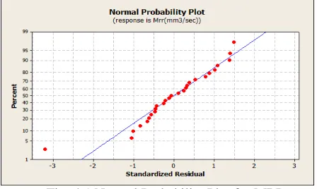
4.3.1 Normal Probability Plot For MRR
The normal probability plotin the Fig:4.1 shows
a clear pattern (as the points are almost in a straight line) indicating that all the factors and their interaction given in are affecting the MRR. In addition, the errors are normally distributed and the regression model is well fitted with the observed values.
Fig: 4.1 Normal Probability Plot for MRR
4.3.2 Standardized Residual Vs Fitted Value for MRR
Fig: 4.2 indicate that the maximum variation
which shows the high correlation that exists between fitted values and observed values.
Fig: 4.2 Residual Vs Fitted Value For MRR
4.3.3 Effect of Input Parameters
450 350 250 30
25
20
15
10
1.00 0.75
0.50 0.1 0.2 0.3
Speed
M
ea
n
of
M
RR
Feed DOC
Main Effects Plot for MRR
Fitted Means
All displayed terms are in the model.
Fig: 4.3 Main Effects plot for MRR
4.3.4 Interaction Effects
40 30 20 10
500 400 300 200 40 30 20 10
1.00 0.75
0.50 Speed * Feed
Speed * DOC
Speed
Feed * DOC
Feed
0.5 0.75 1 Feed
0.1 0.2 0.3 DOC
M
ea
n
of
M
RR
Interaction Plot for MRR
Fitted Means
All displayed terms are in the model.
Fig: 4.4 Interaction Effects plot for MRR
Table 4.1 Comparison of calculated and predicted values of MRR S.
no Spee
d (rpm
)
Feed (mm/r ev)
Depth of cut (mm)
MRR (mm3
MRR (mm / sec) (Expt)
3
% Error /se
c) (Predict
d)
1 500 0.75 0.2 11.3 10.98 2.831
2 500 1 0.1 13.9 12.75 8.273
3 200 0.75 0.3 14.5 14.12 2.62
4 300 0.75 0.2 14.3 13.87 3
5 200 0.5 0.2 8.7 9.18 -5.51
6 300 1 0.2 22.5 21.45 4.66
7 200 0.5 0.1 8.37 8.52 -1.79
8 300 0.75 0.3 22.3 24.35 -9.19
9 300 0.5 0.2 13.2 11.98 9.24
10 500 0.5 0.2 29.4 31.02 -5.05
11 200 1 0.3 22.7 21.45 5.5
777
Copyright © 2011-15. Vandana Publications. All Rights Reserved.
13 200 1 0.2 17.4 15.99 8.1
14 500 0.5 0.3 35.2 33.96 3.52
15 300 0.75 0.1 14.6 15.83 -8.42
16 500 0.5 0.1 14.6 16.32 -11.78
17 500 0.75 0.3 46.4 44.53 4.03
18 200 1 0.1 5.6 5.02 1.03
19 300 0.5 0.3 20.2 18.11 10.34
20 300 1 0.1 12.9 13.78 -6.82
21 500 1 0.2 36.5 34.93 4.3
22 300 0.5 0.1 12.9 13.76 -6.66
23 500 0.75 0.1 12.3 11.55 6.09
24 200 0.75 0.1 7.09 6.81 3.94
25 200 0.75 0.2 16.2 17.66 -9.01
26 200 0.5 0.3 17.2 15.89 7.61
27 300 1 0.3 30.7 33.45 -8.95
4.4 Mathematical Relationship between the Input Parameters and Surface Roughness
The mathematical relationship for correlating the Metal removal rate and the considered process variables has been obtained as follows
Surface roughness =
5.85319-0.47389×A-0.09089×B-0.25012×C+0.411958×A2+0.19167×B2-0.38833×C2
-0.17304×AB-0.17607×AC+0.31500×BC
Where, A is Spindle Speed B is Feed
C is Depth of Cut
4.4.1 Normal Probability Plot For Ra
The normal probability plot as shown in
Fig:4.5 represents a clear pattern (as the points
are almost in a straight line) indicating that all
the factors and their interaction given in are
affecting the Ra. In addition, the errors are normally distributed and the regression model is well fitted with the observed values
Fig: 4.5 Normal Probability Plot For Ra
4.3.2 Standardized Residual Vs Fitted Value for Surface Roughness
Fig:4.6 indicates that the maximum variation
which shows the high correlation that, exists between fitted values and observed values.
Fig: 4.6 Residual Vs Fitted Value for Surface Roughness
4.3.3 Effect of Input Parameters
450 350 250 6.8 6.6 6.4 6.2 6.0 5.8 5.6 5.4 5.2 5.0
1.00 0.75
0.50 0.1 0.2 0.3
Speed
M
ea
n
of
R
a
Feed DOC
Main Effects Plot for Ra
Fitted Means
All displayed terms are in the model.
Fig: 4.7 Main Effects plot for Surface Roughness
4.3.4 Interaction Effects
7.0 6.5 6.0 5.5 5.0
500 400 300 200 7.0 6.5 6.0 5.5 5.0
1.00 0.75
0.50 Speed * Feed
Speed * DOC
Speed
Feed * DOC
Feed
0.5 0.75 1 Feed
0.1 0.2 0.3 DOC
M
ea
n
of
R
a
Interaction Plot for Ra
Fitted Means
All displayed terms are in the model.
778
Copyright © 2011-15. Vandana Publications. All Rights Reserved.
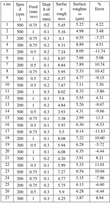
Table 5.8 Comparison of calculated and predicted values
of Surface roughness
4.4 Optimization Plot:
A Minitab Response Optimizer tool shows how different experimental settings affect the predicted responses for factorial, response surface, and mixture designs. Minitab calculates an optimal solution and draws the plot as shown in Fig:4.9. The optimal solution serves as the starting point for the plot. This allows to interactively changing the input variable settings to perform sensitivity analyses and possibly improve the initial solution.
Fig: 4.9 Optimisation plot for MRR and Surface Roughness
The optimization plot as shown in Fig: 4.6 signifies the affect of each factor (columns) on the responses or composite desirability (rows). The vertical red lines on the graph represent the current factor settings. The numbers displayed at the top of a column show the current factor level settings (in red). The horizontal blue lines and numbers represent the responses for the current factor level. Minitab calculates the maximum metal removal rate and minimum surface roughn ess.
From the optimization plot it can be said that the maximum metal removal rate is 53.8838 mm3
This paper produces a direct equation with the combination of controlled parameters which can be used
/sec and the minimum surface roughness is 5.2271µm obtained when spindle speed=500 rpm, feed=1.0mm/rev, and depth of cut=0.3mm.
V. CONCLUSION
In the present work, Multi-Response Optimization problem has been solved by using an optimal parametric combination of input parameters such as Spindle speed, Feed and Depth of Cut. These optimal parameters ensures in producing high surface quality turned product.
Response Surface Methodology is successfully implemented for optimizing the input parameters.
s.no Spee
d (rpm
)
Feed (mm /rev)
Dept h of cut( mm)
Surfac e rough
ness
Surface roughne
ss
(μm)
% Error
1 500 0.75 0.2 5.45 5.22 4.22
2 500 1 0.1 5.16 4.98 3.48
3 200 0.75 0.3 6.1 6.55 -7.37
4 300 0.75 0.2 9.31 8.89 4.51
5 200 0.5 0.2 7.24 8.09 -11.74
6 300 1 0.2 8.07 7.66 5.08
7 200 0.5 0.1 8.84 7.89 10.74
8 300 0.75 0.3 5.95 5.33 10.42
9 300 0.5 0.2 4.37 4.77 -9.15
10 500 0.5 0.2 7.67 7.11 7.30
11 200 1 0.3 8.02 8.33 -3.86
12 500 1 0.3 5.8 5.55 4.31
13 200 1 0.2 4.84 5.26 -8.67
14 500 0.5 0.3 3.93 4.31 -9.66
15 300 0.75 0.1 3.38 2.99 11.5
16 500 0.5 0.1 5.97 6.36 -6.53
17 500 0.75 0.3 5.5 6.14 -11.63
18 200 1 0.1 8.08 7.22 10.60
19 300 0.5 0.3 5.94 6.28 -5.72
20 300 1 0.1 6.08 6.35 -4.44
21 500 1 0.2 4.26 3.91 8.21
22 300 0.5 0.1 5.99 5.33 11.01
23 500 0.75 0.1 7.27 6.54 10.04
24 200 0.75 0.1 4.77 5.15 -7.96
25 200 0.75 0.2 5.75 6.13 -6.60
26 200 0.5 0.3 5.9 6.28 -6.44
779
Copyright © 2011-15. Vandana Publications. All Rights Reserved.
in industries to know the Values of MRR and Surface Roughness instead of machining.
Hence the optimal solution for Metal Removal Rate and Surface Roughness were obtained as 53.8838 mm3/sec and 5.2271µm respectively when spindle speed=500rpm,Feed=1.0mm/rev and depth of cut=0.3mm.
From the graphs it was inferred that the Surface Roughness is effected by speed and depth of cut. Similarly Metal removal Rate is effected by speed, feed, depth of cut.
REFERENCES
[1] H. Yanda, J.A. Ghani, M.N.A.M. Rodzi, K. Othman and C.H.C. Haron, Optimization Of Material Removal Rate, Surface Roughness And Tool Life On Conventional Dry Turning Of Fcd700, International Journal of Mechanical and Materials Engineering (IJMME), Vol.5 (2010), No.2, 182-190.
[2] Dr. M. Naga Phani Sastry, K. Devaki Devi, Dr, K. Madhava Reddy, Analysis and Optimization of Machining Process Parameters Using Design of Experiments, Industrial Engineering Letters, ISSN 2224-6096 (Paper) ISSN 2225-0581 (online) Vol 2, No.9, 2012
[3] D.Martin Suresh Babu, M.Senthilkumar, J.Vishnu, Optimization of cutting parameters for CNC turned parts using Taguchi's technique, International Journal of Engineering, 10(3), 2012, pp.493-496. [ISSN: 1584-2673]
[4] H.Ganesan, Optimization Of Machining Parameters In Turning Process Using Genetic Algorithm And Particle Swarm Optimization With Experimental Verification, International Journal of Engineering Science & Technology;2011, Vol. 3 Issue 2, p1091
[5] Buragohain, M. and Mahanta, C. ‘A novel approach for ANFIS modeling based on full factorial design’, Applied Soft Computing, Vol. 8,2008, pp.609–625.