Analysis of the M
/
M
/
1 queue with single working vacation and vacation
interruption
Shakir Majid∗, P.Manoharan
Department of Mathematics Annamalai University, Annamalainagar-608002, Tamil Nadu, India.
Abstract
In this work, a vacation interruption in M/M/1 queue with single working vacation is considered. Using the matrix analytic method, we obtain the distributions for the mean queue length and the mean sojourn time and their stochastic decomposition structures. Finally, we demonstrate the effects of system parameters on the performance measures and present some special cases.
Key words: M/M/1 queue, Vacation, Working vacation, Stochastic decomposition, Matrix-geometric solution. AMS classification: 60K25, 68M20
1. Introduction
Queuing systems with vacations have been studied extensively by various researchers for their profound appli-cations in many real life situations such as telecommunication, computer networks, production systems, and so on. The details have been reported in the survey of Doshi (1986), the monographs of Takagi (1991) and Tian and Zhang (2006). In these studies, it is assumed that the customers service is completely stopped during a vacation. However, there are numerous examples, where the server serves the customers at a lower rate during a vacation, rather than being completely inactive. This type of semi vacation policy was first introduced by Servi and Finn (2002). This type of vacation policy is called a working vacation (WV). Servi and Finn (2002) analyzed M/M/1 queue with multiple working vacation policy and derived the PGF of the queue length and LST of the waiting time, and utilized their results to analyze the system performance of gateway router in fiber communication networks. Later M/M/1 with multiple working vacation model was also studied by Liu, Xu and Tian (2007) to obtain explicit expressions of the performance measures and their stochastic decomposition by using the matrix-geometric method. Subsequently, by applying the same method, M/M/1 queue with single working vacation was analyzed by Tian and Zhao (2008) and obtained various steady state indicators. Kim, Choi and Chae (2003), Wu and Takagi (2006) and Li et al. (2011) ex-tended the study in Servi and Finn (2002) to an M/G/1/WV queue. Baba (2005) applied the matrix-geometric solution method to generalize the work of Servi and Finn (2002) to a GI/M/1 queue with general arrival process and multiple working vacations. Later, Li and Tian (2011) investigated the GI/M/1 queue with single working vacation.
Situations often arise where the server must stop the vacation and come back to normal working level, once some system indices, such as the number of customers, attain a certain value during a vacation. In many real life scenarios, important events happen during a vacation and the server rather than continuing to take residual vacation must return to normal work. For example, when the number of waiting customers in the system exceeds a certain value during a vacation and server continues to be in vacation, it leads to a large cost of waiting customers. Hence the server vacation interruption is more effective and reasonable to vacation queues. Li and Tian (2007) first studied the vacation interruptions in an M/M/1 queuing model with working vacation and derived the steady state distributions of the expected queue length and expected waiting time along with stochastic decomposition structures in terms of
matrix-IThis research did not receive any specific grant from funding agencies in the public, commercial, or not-for-profit sectors.
∗corresponding author
geometric method. Later, Li and Tian (2007) and Li et al. (2008) generalized this work to GI/Geo/1 and GI/M/1 queue by using matrix-analytic method. Zhang and Hou (2010) analyzed the vacation interruptions in M/G/1 queue with working vacation by utilizing the method of supplementary variable. They obtained the queue length distribution and LST of the stationary waiting time. Zhang and Hou (2011) extended the work of Zhang and Hou (2010) to an MAP/G/1/WV queue and computed the system size distribution and the Laplace-Stieltjes transform (LST) of waiting time. Later, Gao et al. (2014) analyzed the M/G/1/MWV queue with retrials. Laxmi and Jyothsna (2015) studied the impatient customer in M/M/1 queue under Bernoulli schedule vacation interruption and obtained various performance measures by adopting the PGF method.
In this paper, we consider an M/M/1 queuing system with two vacation policies. The working vacation and vacation interruption are connected and the server takes a working vacation as soon as the system becomes empty and customers are served at the lower rate during the working vacation period. If the system is non empty at the service completion instant during the vacation period, the server will return to the normal busy period no matter whether or not the vacation ends. Otherwise, he continues the vacation until there are customers after a service or a vacation ends. The purpose of our work is to develop a set of stationary performance measures such as the mean queue length and waiting time. With these performance measures, we illustrate the effects of system parameters on the performance indices of the system.
The rest of the paper is organized as follows. In section 2, we describe the model as a quasi-birth death process. In section 3, we obtain the steady state distribution of the queue length and the state probabilities of the server. Section 4 discusses the stochastic decomposition structures of the queue length and sojourn time, and obtains the distributions of the additional queue length and additional delay.Finally the numerical examples are presented in section 5.
2. Model description
Consider a classical M/M/1 queuing system with Poisson arrival rateλand a service rateµ. The server begins a working vacation as soon as the system becomes empty and the vacation period V follows an exponential distribution with the parameterφ. During a vacation period, the arriving customers are served at an exponential rateη, where
η < µ. The server is assumed to interrupt the vacation if there are customers in the system at a service completion instant during a working vacation period and changes its service rate fromη toµ, thereby giving rise to a normal working level. Otherwise, the server continues the working vacation until the system is non empty after the service or a vacation ends. Meanwhile, if the server finds no customer in the system after returning from the working vacation, he does not take another vacation but stays idle until the next arrival. In this service discipline, the server may return from the vacation without completing it and can stay in the vacation period if the system is empty at the instant of a service completion. Meanwhile, the vacation service rate is applicable only to the first customer arrived during a vacation period. The inter-arrival times, the service times, and the working vacation times all are taken to be mutually independent. In addition, the service order is first in first out (FIFO).
Let L(t) be the number of customers in the system at time t and J(t) be the status of the server, which is defined as follows:
J(t)=
0 When the server is in WV period at time t,,
1 When the server is in normal working period at time t,
Then{(L(t),J(t)),t≥0}defines a continuous time Markov chain with state space
S ={(k,j) :k=0,1,2, ...,j=0,1}
Using the lexicographical order for the states, the infinitesimal generator is given by
Q=
A0 C
B1 A C
B A C B A C
.. . ... ...
Where A0= −(λ0+φ) −λφ
!
, C= λ 0
0 λ
!
, B1 = ηµ 00
! ,
A= −(λ+0φ+η) −(λφ+µ) !
, B= 00 µη !
,
The matrix structure of Q indicates that the Markov Chain{(L(t),J(t)),t≥0}is a quasi birth and death process. To analysis the QBD process, we first need to get the rate matrix, denoted by R, which is the minimal non-negative solution of the matrix quadratic equation
R2B+RA+C=0 (1)
The following lemma presents the explicit solution of R. Lemma 1.Ifλ
η <1, the minimal non-negative solution of matrix quadratic equation (1) has the following expression:
R= r ρ
λ+φ λ+φ+η
0 ρ
!
(2)
r= λ
λ+φ+η (3)
Proof.Since A, B and C in (1) are all upper triangular matrices, therefore we can consider that the solution matrix R has the same structure as
R= r11 r12 0 r22
!
Substituting the matrix value R into (1) leads to
−(λ+φ+η)r11+λ=0
µr222 −(λ+µ)r22+λ=0 (4)
ηr2
11+µr12(r11+r22)+φr11−(λ+µ)r12=0
We can obtain the minimal non-negative solution of (1) from the above set of equations, by using the fact thatµz2− (λ+µ)z+λ=0 has a unique rootr22 =ρin interval (0,1).Substitutingr11 =randr22 =ρinto the last equation of (4), we getr12=ρλλ++φφ+η, then the proof is complete.
According to the expression of R in Neuts (1981, Theorem 3.1.1) and lemma 1, it is easy to prove that the QBD process{(L(t),J(t)),t≥0}is positive recurrent if and only ifρ <1.
3. Stationary distribution of queue length
Ifρ <1, let (L,J) be the stationary limit of the QBD process{(L(t),J(t)),t≥0}and define
πk=(πk0, πk1), k≥0
πk j=P{L=k,J= j,t≥0}=lim
t→∞{(L(t)=k,J(t)= j}, (k,j)∈S,
Theoem 1.Ifρ <1, the Stationary probability distribution of (L,J) is
πk0=Krk, k≥0,
π01 =Kφ
λ (5)
πk1=K
λρ(+λφ++φ)η k−1
X
j=0
ρjrk−1−j+φ
µρ
K−1
, k≥1
Where
K=(1−r)(1−ρ) "
(1−ρ)+φ
λ(1−r)(1−ρ)+
ρ(λ+φ)
λ+φ+η + φ µ(1−r)
#−1
(6)
Proof.Using the matrix geometric solution method by Neuts (1981), we get
πk=(πk0, πk1)=(π10, π11)Rk−1, k≥1 (7)
and (π00, π01, π10, π11) satisfies the following set of equations
(π00, π01, π10, π11)B[R]=0 (8)
Where
B[R]= AB0 C
1 RB+A
! =
−(λ+φ) φ λ 0
0 −λ 0 λ
η 0 −(λ+φ+µ) (λ+φ)
µ 0 0 −µ
Substituting B[R] into (8), we obtain the set of equations as follows
−(λ+φ)π00+ηπ10+µπ11=0
φπ00−λπ01=0
λπ00−(λ+φ+η)π10=0 (9)
λπ01−(λ+φ)π10−µπ11 =0 Takingπ00 =Kand solving the above equations in terms of K, we obtain
π10 =Kr, π01=kφλ, π11=K
hρ(λ+φ)
λ+φ+η + φ µ
i
From (2), we obtain
Rk=
rk ρ(λ+φ) λ+φ+ηρ
kP−1 j=0ρ
jrk−1−j
0 ρk
, k≥1 (10)
Substituting (π10, π11) and the matrix expressionRk−1into (7), we obtain (5) and noting that constant factor K can be determined by utilizing the normalization condition.
From theorem 1, the probabilities that the system is in working vacation period, idle period and regular busy period are obtained as follows,respectively:
P{J=0}=
∞
X
k=0
πk0=K0(1−ρ)
P{the server is in idle period}=Kφ
λ (11)
P{J=1}=
∞
X
k=1
πk1=K0(1−r)
"
ρ(λ+φ) (λ+φ+η)(1−r)+
φ µ
#
Where
K0 =
"
(1−ρ)+φ
λ(1−r)(1−ρ)+
ρ(λ+φ)
λ+φ+η+ φ µ(1−r)
#−1
(12)
4. Stochastic decompositions
To achieve a better comparison with the queuing models already existing, we often attempt to decompose the quantities of interest into various factors. In vacation queuing models, the stochastic decomposition structures plays a significant role and underlines the influence of system vacation on system performance indices such as mean queue length and mean sojourn times. For the system under investigation, we strive to do a similar decomposition.
Theoem 2. If ρ < 1 andη > µ, the stationary queue length L in system can be decomposed into sum of two independent random variables: L = L0+Ld, whereL0 is the stationary queue length of the classical M/M/1 queue
without vacation and follows a geometric distribution with parameter 1-ρand the additional queue lengthLd has a modified geometric distribution
P{Ld=K}=
K∗λ+φ
λ (1−r), K=0
K∗r−ρ+rλ+φ µ
(1−r)rK, K≥1 (13)
Where K∗= K
(1−r)(1−ρ) = "
λ+φ
λ (1−r)+r−ρ+r λ+φ
µ
#−1
(14)
Proof.By theorem 1, the PGF of L can be expressed as follows
L(z)=
∞
X
k=0 πk0zk+
∞
X
k=0
πk1zk=K
"
φ λ+
1 1−rz+
ρ(λ+φ)
λ+φ+η
z
(1−rz)(1−ρz)+
φ µ
z 1−ρz
#
= 1−ρ
1−ρzK
∗
"
φ
λ(1−r)(1−ρz)+
1−r
1−rz(1−ρz)+
ρ(λ+φ)
λ+φ+η
z(1−r) (1−rz)+
φ µ(1−r)z
#
Note that
φ λρ=
φ µ,
1−r
1−rz(1−ρz)=(1−r)+(r−ρ) z(1−r)
1−rz HenceL(z) can be rewritten as
L(z)= 1−ρ 1−ρzK
∗
"
λ+φ
λ (1−r)+ r−ρ+
r(λ+φ)
µ
! z(1−r)
1−rz #
=L0(z)Ld(z) (15)
where
K∗=
"
(1−ρ)+φ
λ(1−r)(1−ρ)+
ρ(λ+φ)
λ+φ+η+ φ µ(1−r)
#−1
= "
1−r+φ
λ(1−r)(1−ρ)+r−ρ+
ρ(λ+φ)
λ+φ+η+ φ µ(1−r)
#−1
= "
λ+φ
λ (1−r)+r−ρ+r λ+φ
µ
#−1
ExpandingLd(z) in power series of z, we get (13).
Theorem 2 shows that the additional queue lengthLd(z) is a mixture of two random variables
i.e Ld=K∗(λ+φ)(1−r)
λ X0+K
∗(r−ρ+r(λ+φ)
µ )X1 (16)
WhereX0=0 andX1follows the geometric distribution with parameter 1-r. Based on stochastic decomposition in theorem 2, we obtain
E(Ld)=K∗
"
r−ρ+rλ+φ
µ
# 1
1−r (17)
E(L)= ρ 1−ρ+K
∗
"
r−ρ+rλ+φ
µ
# 1
1−r (18)
Theoem 3. Ifρ < 1 andµ > η, the stationary sojourn time S of an arrival can be decomposed into the sum of two independent variables: S =S0+Sd, whereS0is the sojourn time of an arrival in a corresponding classical M/M/1 queue and is exponentially distributed with parameterµ−λandSdis the additional delay with the LST given by
S∗
d(s)=K∗
(λ+φ
λ )(1−ρ)−
r−ρ
r
(1−r)+ "
r−ρ
r +
λ+φ µ
# λ r −λ λ r −λ+s
Where
K∗="(λ+φ
λ )(1−ρ)−
r−ρ
r
(1−r)+r−ρ r +
λ+φ µ
#−1
Proof.The classical relation between the PGF of a queue length L and the LST of sojourn time S by Keilson and Sevi (1988) is given as follows
L(z)=S∗(λ(1−z))
From theorem 2, we get
L(z)= 1−ρ 1−ρzK
∗
" (λ+φ
λ )(1−r)+ r−ρ+
r(λ+φ)
µ
! z(1−r)
1−rz #
(20)
Takingz=1− s
λin (20) and noting that
1−ρ
1−ρz =
µ(1−ρ)
µ(1−ρ)+s,
1−r 1−rz =
λ r −λ λ r −λ+s We obtain
S∗(s)= µ(1−ρ)
µ(1−ρ)+sK
∗
(λ+φ
λ )(1−r)+(r−ρ+
r(λ+φ)
µ )(1−
1 r +
1 r
λ r −λ λ r −λ+s
)
= µ(1−ρ)
µ(1−ρ)+sK
∗
(λ+φ
λ −
λ+φ
µ −
r−ρ
r )(1−r)+( r−ρ
r + (λ+φ)
µ )( λ r −λ λ r −λ+s
)
= µ(1−ρ)
µ(1−ρ)+sK
∗
(λ+φ
λ )(1−ρ)−
r−ρ
r
(1−r)+ "
r−ρ
r +
λ+φ µ
# λ r −λ λ r −λ+s
= µ(1−ρ)
µ(1−ρ)+sS
∗
d(s) (21)
From (14), we have
K∗= "
λ+φ
λ (1−r)+r−ρ+r λ+φ
µ
#−1
= "
λ+φ
λ (1−r)+r−ρ+(r+1−1) λ+φ
µ
#−1
(22)
= "
(λ+φ
λ )(1−ρ)−
r−ρ
r
(1−r)+r−ρ r +
λ+φ µ
#−1
(23)
Hence, this verifies thatS∗
d(s) is a LST.
Similarly, theorem 2 indicates that the additional sojourn timeS∗
d(s) is a mixture of two random variables
S∗
d(s)=K∗ (
(λ+φ
λ )(1−ρ)−
r−ρ
r
Y0+
" r−ρ
r +
λ+φ µ
# Y1
)
(24)
WhereY0=0 andY1follows the exponential distribution with parameterλr −λ.
Based on the above stochastic decomposition structure, we get easily obtain the means as follows
E(Sd)=K∗ "
r−ρ+rλ+φ
µ
# 1
λ(1−r) = 1
λE(Ld) (25)
E(S)= 1
µ(1−ρ)+K
∗
"
r−ρ+rλ+φ
µ
# 1
λ(1−r) (26)
5. Numberical Results
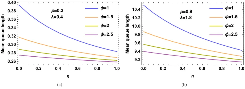
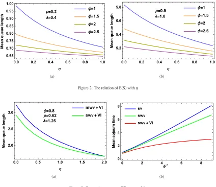
In this section, we provide some numerical examples to demonstrate the above obtained results and discuss the influence of system parameters on system performance indices. Figs 1 and 2 shows how the mean queue length and mean sojourn time respectively changes with the vacation service rateηat different values ofφ. Fig.3(a) illustrates the comparison of mean queue length in our model withM/M/1/MWV+VI(Li and Tian, 2007). Fig.3(b) demonstrates the effect of the mean vacation time on the mean sojourn time and presents the comparison of the mean sojourn time in our model with two different vacation policies i.e the single vacation (SV) and the single working vacation (SWV). The main findings in this study are itemized as
• From fig.1(a), evidently as we increase the value ofη, the mean queue length decreases. Also, we find that the mean queue length depends on the vacation rateφi.e whenη is fixed and ifφis smaller, E(L) is bigger. Meanwhile, the vacation rateφhas a small effect on the mean queue length, when the vacation rateφincreases to a certain value. Furthermore, Fig.1(b) indicates that ifρis larger, the mean queue length E(L) is also larger and this is reasonable in practice. Hence the traffic intensityρalso has some effects on E(L). Fig.2 illustrates that the mean sojourn time E(S) decreases along with the increase of theηand it also decreases ifφis bigger.
• From 3(a), our model gives significantly a better performance in terms of E(L). For example, obviously, when the vacation service rateηare the same in two situations, expected queue length in M/M/1 with SWV and VI is smaller than that in M/M/1 with MWV and VI and the later causes more jobs or customers to wait. Hence, we can achieve a better service under working vacation if we consider vacation interruption policy that utilizes the server and decreases the waiting time effectively.
• From fig.3(b), the E(S) increases with an increase of mean vacation rateφ−1and E(S) reaches to a fixed value, Whenφ−1 tends to zero i.e our system is reduced to a classical M/M/1 queue. Further, the SWV+VI policy gives a better performance as compared to the SV policy and the SWV policy. This is illustrated by the fol-lowing: higher is the probability that vacation interruption occurs if the mean vacation time is longer. In other words, the server will come back more frequently to a normal working level if the mean vacation time is longer. As a result, the server serves more customers at a normal service rate.
(a) (b)
Figure 1: The relation of E(L) withη
(a) (b)
Figure 2: The relation of E(S) withη
(a) (b)
Figure 3: Comparisons among different models .
References
Doshi,B.T., 1986. Queueing systems with vacations-A survey, Queueing Syst. 1, 29-66.
Takagi,H., 1991. Queueing Analysis: A Foundation of Performance Evaluation. Vol. 1: Vacation and Priority Systems, Part1, North-Holland Elsevier, New York.
Tian,N.,Zhang,Z.G., 2006. Vacation Queueing Models-theory and Application. Springer, New York. Servi,L.D.,Finn, S.G., 2002. M/M/1 queues with working vacation (M/M/1/WV). Perform. Eval. 50, 41-52.
Liu, W.,Xu,X.,Tian,N.,2007. Stochastic decompositions in the M/M/1 queue with working vacations. Oper. Res. Lett. 35, 595-600. Tian,N.,Zhao,X., 2008. The M/M/1 queue with single working vacation. Int. J. Inf. Manage. Sci. 19(4), 621-634.
Kim, J.D.,Choi, D.W.,Chae,K.C., 2003. Analysis of queue-length distribution of the M/G/1 queue with working vacation. Hawaii Interna-tional Conference on Statistics and Related Fields.
Wu, D.,Takagi,H., 2006. M/G/1 queue with multiple working vacations. Perform. Eval. 63, 654-681.
Li,J.,Tian, N.,Zhang,Z.G.,Luh,H.P, 2011. Analysis of the M/G/1 queue with exponentially working vacationsa matrix analytic approach. Queueing Syst. 61, 139-166.
Baba,Y., 2005. Analysis of a GI/M/1 queue with multiple working vacations. Oper. Res. Lett. 33, 201-209.
Li,J.,Tian, N., 2011. Performance analysis of an GI/M/1 queue with single working vacation. Appl. Math. Comput. 217, 4960-4971. Li, J., Tian, N., 2007. The M/M/1 queue with working vacations and vacation interruptions. Journal of System Sciences and Systems Engi-neering 16(1), 121-127.
Li, J., Tian, N., 2007. The discrete-time GI/Geo/1 queue with working vacations and vacation interruption. Applied Mathematics and Com-putation 185(1), 1-10.
Li, J., Tian, N., Ma, Z., 2008. Performance analysis of GI/M/1 queue with working vacations and vacation interruption. Applied Mathematical Modelling 32(12), 2715-30.
Zhang, M., Hou, Z., 2010. Performance analysis of M/G/1 queue with working vacations and vacation interruption. Journal of Computational and Applied Mathematics 234(10), 2977-85.
Gao, S., Wang, J., Li, WW., 2014. An M/G/1 retrial queue with general retrial times, working vacations and vacation interruption. Asia-Pacific Journal of Operational Research 31(2), article no. 1440006.
Zhang, M., Hou, Z., 2011. Performance analysis of MAP/G/1 queue with working vacations and vacation interruption. Applied Mathematical Modelling 35(4), 1551-60.
Laxmi, PV., Jyothsna, K., 2015. Impatient customer queue with Bernoulli schedule vacation interruption. Computers and Operations Research 56, 1-7.
Neuts,M., 1981. Matrix-Geometric Solution in Stochastic Model, Hopkins University Press, Baltimore. Keilson,J.,Sevi,L.D., 1988. A distribution form of Littles law, Oper. Res. Lett. 7(5), 223-227.