The Thirty-Third AAAI Conference on Artificial Intelligence (AAAI-19)
Natural Option Critic
Saket Tiwari
College of Information and Computer Sciences University of Massachusetts Amherst
Amherst, MA 01003 [email protected]
Philip S. Thomas
College of Information and Computer Sciences University of Massachusetts Amherst
Amherst, MA 01003 [email protected]
Abstract
The recently proposedoption-criticarchitecture (Bacon, Harb, and Precup 2017) provides a stochastic policy gradient ap-proach to hierarchical reinforcement learning. Specifically, it provides a way to estimate the gradient of the expected dis-counted return with respect to parameters that define a finite number of temporally extended actions, calledoptions. In this paper we show how the option-critic architecture can be extended to estimate thenaturalgradient (Amari 1998) of the expected discounted return. To this end, the central questions that we consider in this paper are: 1)what is the definition of the natural gradient in this context,2)what is the Fisher information matrix associated with an option’s parameterized policy,3)what is the Fisher information matrix associated with an option’s parameterized termination function, and4)
how can acompatible function approximationapproach be leveraged to obtain natural gradient estimates for both the pa-rameterized policy and papa-rameterized termination functions of an option with per-time-step time and space complexity linear in the total number of parameters. Based on answers to these questions we introduce the natural option critic algo-rithm. Experimental results showcase improvement over the
vanilla gradientapproach.
Introduction
Hierarchical reinforcement learning methods enable agents to tackle challenging problems by identifying reusableskills— temporally extended actions—that simplify the task. For example, a robot agent that tries to learn to play chess by reasoning solely at the level of how much current to give to its actuators every 20ms will struggle to correlate obtained re-wards with their true underlying cause. However, if this same agent first learns skills to move its arm, grasp a chess piece, and move a chess piece, then the task of learning to play chess (leveraging these skills) becomes tractable. Several mathe-matical frameworks for hierarchical reinforcement learning have been proposed, includinghierarchies of machines(Parr and Russell 1998), MAXQ (Dietterich 2000), and the options framework (Sutton, Precup, and Singh 1999). However, none of these frameworks provides a practical mechanism forskill discovery: determining what skills will be useful for an agent to learn. Although skill discovery methods have been pro-posed, they tend to beheuristicin that they find skills that
Copyright c2019, Association for the Advancement of Artificial Intelligence (www.aaai.org). All rights reserved.
have a property that intuitively might make for good skills for some problems, but which do not follow directly from the primary objective of optimizing the expected discounted return (Machado, Bellemare, and Bowling 2017; Simsek and Barto 2008; Thrun and Schwartz 1995; Konidaris and Barto 2009).
Theoption-criticarchitecture (Bacon, Harb, and Precup 2017), stands out from other attempts at developing a gen-eral framework for skill discovery in that it searches for the skills that directly optimize the expected discounted return. Specifically, the option critic uses the aforementioned options framework, wherein a skill is called anoption, and it proposes parameterizing all aspects of the option and then performing stochastic gradient descent on the expected discounted return with respect to these parameters. The key insight that enables the option-critic architecture is a set of theorems that give expressions for the gradient of the expected discounted return with respect to the different parameters of an option.
One limitation of the option critic is that it uses ordinary (stochastic) gradient descent. In this paper we show how the option critic can be extended to usenatural gradient descent (Amari 1998), which exploits the underlying structure of the option-parameter space to produce a more informed update direction. The primary contributions of this work are theo-retical: we define the natural gradients associated with the option critic, derive theFisher information matrices associ-ated with an option’s parameterized policy and termination function, and show how the natural gradients can be esti-mated with per-time-step time and space complexity linear in the total number of parameters. This is achieved by means ofcompatible function approximations. We also analyze the performance of natural gradient descent based approach on various learning tasks.
Preliminaries and Notation
Areinforcement learning(RL) agent interacts with an en-vironment, modeled as aMarkov decision process(MDP), over a sequence of time steps t ∈ N≥0. A finite MDP
is a tuple (S,A, P, R, d0, γ). S is the finite set of
possi-ble states of the environment. St is the state of the envi-ronment at time t. Ais the finite set of possible actions the agent can take. At is the action taken by the agent at timet. P :S × A × S → [0,1]is the transition function:
P(s, a, s0)the probability of transitioning to states0given the agent takes actionain states.Rtdenotes the reward at timet. Ris thereward function,R : S × A →R, where
R(s, a) =E[Rt|St=a, At=a], i.e., the expected reward the agent receives given it took actionain states. We say that a process has ended when the environment enters a termi-nal state, meaning for a terminal states,P(s, a, s0) = 0and
R(s, a) = 0for alls0∈ S \{s}anda∈ A. The process ends afterT steps and we callT thehorizon. We say the process isinfinite horizonwhen there does not exist a finiteT. d0
is the initial state distribution, i.e.,d0(s) = Pr(S0=s). The parameterγ∈[0,1]scales how the rewards are discounted over time. When a terminal state is reached, time is reset to
t= 0and consequently a new initial state is sampled using
d0.
A policy, π : S × A → [0,1], represents the agent’s decision making system: π(s, a) = Pr(At=a|St=s). Given a policy, π, and an MDP, (S,A, P, R, d0, γ), an
episode, H is a sequence of states of the environment, actions taken by the agent, and the rewards observed from the initial state, S0, to the terminal state, ST, i.e.,
H = (S0, A0, R0, S1, A1, R1, ..., ST, AT, RT). We also define the path that an agent takes to be a sequence of states and actions, i.e., a history without rewards, X = (S0, A0, S1, A1, ..., ST, AT). PathX is a random variable from the set of all possible paths,X. The return of an episode
His the discounted sum of all rewards,g(H) =PTt=0γtR t. We callvπthe value function for the policyπ,vπ:S →R, where vπ(s) = E[PTt=0γ
tRt|, S0=s, π]. We call q π the action-value function associated with policyπ,qπ:S ×A →
R, whereqπ(s, a) =E[PTt=0γ
tRt|S0=s, A0=a, π].
Policy Gradient Framework
Thepolicy gradient framework(Sutton et al. 1999; Konda and Tsitsiklis 2000) assumes the policyπ, parametrized by
θ, is differentiable. The objective function, ρ, is defined with respect to a start states0,ρ(θ) =E[PTt=0γ
tRt|d
0, θ].
The agent learns by updating the parametersθapproximately proportional to the gradient∂ρ/∂θ, i.e.,θ←α∂ρ/∂θwhere
αis thelearning rate(LR): a scalar hyper-parameter.
Option Critic framework
Theoptions framework(Sutton, Precup, and Singh 1999) formalizes the notion of temporal abstractions by introducing options. An option,o, from a set of options,O, is a gener-alization of primitive actions. The intra-option policyπo : S × A →[0,1]represents the agent’s decision making while executing an optiono: πo(s, a) = Pr(At=a|St=s, Ot=o). Like primitive actions the agent executes an option at a state
St and the option terminates at another St+τ, whereτ is the duration for which the agent is executing the option:ot. While in the optiono, from stateSttoSt+τ, the agent fol-lows the policy πo. Optiono terminates stochastically in statesaccording to a distributionβ. The framework puts restrictions on where an option can be initiated by defining an initiation state set,Io, for optiono. The optionois initi-ated in states∈ Iobased onπO(s), which is a policy over options defined asπO :S × O →[0,1]. An initiation state
setIo, an intra-option policyπoand a termination function
βo : S → [0,1]comprise an optiono. It is commonly as-sumed that all options are available everywhere and thereby we dispense with the notion of an initiation set.
Theoption critic frameworkmakes all the options available everywhere, and introduces policy-gradient theorems within the options framework. The option active at time steptisOt. The intra-option policies (πo) and termination functions (βo) are represented using differentiable functions parametrized byθandϑ, respectively. The goal is to optimize the expected discounted return starting at states0and optiono0. We
re-define the objective function,ρ, for the option critic setting:
ρ(O, θ, ϑ, s, o) =E[P∞t=0γtRt|O, θ, ϑ, S0=s, O0=o].
Equations similar to those in the policy gradient framework (Sutton et al. 1999) are manipulated to derive gradients of the objective with respect toθandϑin the option-critic frame-work. The analogous state value function isvπO :S →R,
where vπO(s) = E[
P tγ
tRt|S0=s]. v
πO(s)is the value
of a state s, within the options framework, with the op-tion set O and the policy over options πO. The option-value function isqπO : S × O → R, whereqπO(s, o) =
E[Ptγ
tRt|S0=s, O0=o]. Here, q
πO(s, o)is the value of
stateswhen optionois active with the option setO. The state-option-action value function isqU : S × O × A → R, where qU(s, o, a) = E[Ptγ
tRt|S0=s, O0=o, A0=a].
Here, qU(s, o, a)is the value of executing actionain the context of state-option pair(s, o). The option-value func-tion upon arrivalis u : O × S → R, where u(o, s0) = E[PtγtRt|S1=s0, O0=o]. Here,u(o, s0)is the value of op-tionobeing active upon the agent entering states0. Bacon, Harb, and Precup (2017) observe a consequence of the defi-nitions:
u(o, s0) = (1−βo(s0))qπO(s
0, o) +β
o(s0)vπO(s
0).
The main results presented by Bacon, Harb, and Pre-cup (2017) are theintra-option policy gradient theoremand thetermination gradient theorem. The gradient of the ex-pected discounted return with respect toθand initial condi-tion(s0, o0)is:
∂qπO(s0, o0)
∂θ =
X
s,o
µO(s, o)
X
a
∂πo(s, a, θ)
∂θ qU(s, o, a),
whereµO(s, o)is the discounted weighting of state-option pair(s, o)along trajectories starting from(s0, o0)defined by:
µO(s, o) =P∞t=0γ
tPr(S
t=s, Ot=o|s0, o0). The gradient
of the expected discounted return with respect toϑand initial condition(s1, o0)is:
∂u(o0, s1)
∂ϑ =−
X
o,s0
µO(s0, o)
∂βo(s0, ϑ)
∂ϑ aO(s 0, o),
where aO : S × O → R is the advantage function over options such that aO(s0, o) = qπO(s
0, o)−v
πO(s
0).
Here, µO(s0, o) is the discounted weighting of state op-tion pair (s0, o)from(s1, o0), i.e., according to a Markov
chain shifted by one time step, defined by: µO(s0, o) =
P∞ t=0γ
tPr(S
t+1=s0, Ot=o|s1, o0). The agent learns by
Meaning, it learns by updatingθ←αθ∂qπO(s0, o0)/∂θand
ϑ ←αϑ∂u(o0, s1)/∂ϑ, whereαθ andαϑare the learning rates forθandϑ, respectively.
Natural Actor Critic
Natural gradient descent (Amari 1998) exploits the under-lying structure of the parameter space when defining the direction of steepest descent. It does so by defining the inner producthx, yiθin the parameter space as:
hx, yiθ=xTGθy, (1) whereGθis called themetric tensor. Although the choice ofGθremains open under certain conditions (Thomas et al. 2016) we choose the Fisher information matrix, as is common practice. The fisher information matrix distribution over random variable X, parametrized by policy parametersθ, that lie on a Reimannian manifold (Rao 1945; Amari 1985):
(Gθ)i,j =E
∂ln Pr(X;θ)
∂θi
∂ln Pr(X;θ)
∂θj
,
where the expectation is over the distribution Pr(X) and
(Gθ)i,jrepresents a matrix with itsi, jthelement being the expression as defined on the right hand side — we use this notation to represent a matrix throughout the paper. Kakade (2001) makes the assumption that every policy,π, is ergodic and irreducible, therefore it has a well-defined sta-tionary distributionfor each states. Under this assumption, Kakade (2001) introduces the use of natural gradient for opti-mizing the expected reward over the parametersθof policy
π, as defined byρ(θ) =P s,ad
π(s)π(s, a, θ)R(s, a). The
natural gradientfor the objective function,ρ, is defined as:
e
∇ρ(θ) =G−θ1∂ρ(θ)
∂θ . (2)
The derivation of a closed form expression forGθ for the parameter space of policyπ, parametrized byθ, is non-trivial as demonstrated for the limiting matrix of the infinite horizon problem in reinforcement learning (Bagnell and Schneider 2003). For a weight vectorwletqˆwbe an approximation of the state action value functionq(s, a), which has the form:
ˆ
qw(s, a) =wT
∂lnπ(s, a, θ)
∂θ .
The mean squared error(w, θ), for a weight vectorwand a given policy parametrized byθ, is defined as:
(w, θ) =X
s,a
dπ(s)π(s, a, θ)(ˆqw(s, a)−qπ(s, a))2,
where dπ(s) = P∞ t=0γ
tPr(S
t=s|π) is the discounted weighting of state sin the infinite horizon problem. The weights dπ(s)normalize to the stationary distribution for statesunder policyπin the undiscounted setting where the MDP terminates at every time steptwith probability1−γ. Theorem 1 as introduced by Kakade (2001) states thatw˜
which minimizes the mean squared error,(w, θ), is equal to the natural gradient as defined in (2).
Kakade (2001) also demonstrates how natural policy gradi-ent performs under the re-scaling of parameters. In addition
to that, Kakade (2001) demonstrates how the natural gradient weights the components of∇eρ(θ)uniformly, instead of using
dπ(s). We also point out that the natural gradient is indepen-dent to local re-parametrization of the model (Pascanu and Bengio 2013) and can be used inonline learning(Degris, Pi-larski, and Sutton 2012). Natural gradients for reinforcement learning (Peters and Schaal; Bhatnagar et al. 2008; 2009; De-gris, Pilarski, and Sutton 2012), as well as more recent work in deep neural networks (Desjardins et al. 2015; Pascanu and Bengio 2013; Thomas, Dann, and Brunskill 2018; Sun and Nielsen 2017) have shown to be effective in learning.
The Option-Critic architecture uses vanilla gradient to learn temporal abstraction and internal policies, which can be less data efficient compared to the natural gradient (Amari 1998). The natural gradient also overcomes the difficulty posed by the plateau phenomena (Amari 2016). We de-rive the metric tensors for the parameters in the option-critic architecture. Computing the complete Fisher information matrix or is expensive. We use a block-diagonal estimate of the Fisher information matrix as has been applied in the past to reinforcement learning (Thomas 2011) and to neural networks (Roux, Manzagol, and Bengio 2008; Ku-rita 1992; Martens 2010; Pascanu and Bengio 2013; Martens and Grosse 2015). Specifically, we estimateGθandGϑ sepa-rately, whereθandϑare the parameters of of the intra-option policy and the option termination function. These are then combined into a(|θ|+|ϑ|)×(|θ|+|ϑ|)sized estimate of the complete Fisher information matrix of the parameter space, where|θ|,|ϑ|represent the size of vectors.
We also provide theoretical justification for the resulting algorithm inspired from the incremental natural actor critic algorithm (Bhatnagar et al. 2007) (INAC) and its extension to include eligibility traces (Morimura, Uchibe, and Kenji 2005; Thomas 2014).
Start State Fisher Information Matrix Over
Intra-Option Path Manifold
We define pathX in the options framework for the infi-nite horizon problem as the sequence of state-option-action tuples: X = (S0, O0, A0, S1, O1, A1, ...). We useX to
denote the set of all paths. We introduce the function
g : X → Rcalled theexpected return over path, where
g(x) = E[PTt=0γ
tRt|x] is the expected return given the
pathx. The goal in a reinforcement learning problem, in the context of the option-critic architecture, is to maximize the discounted return, ρ(O, θ, ϑ, s0, o0). The goal can be
re-written as maximizing J(θ, s0, o0) = PPr(x;θ)g(x).
Where the summation is over allx∈ X starting from(s0, o0)
and the intra-option policies are parametrized byθ. To opti-mize the objectiveJ, we define it over a Riemannian space
Θ, withθ∈Θ. In the Riemannian space the inner product is defined as in (1). The direction of steepest ascent ofJ(θ)in the Riemannian space,Θ, is given byG−θ1∂J(θ)/∂θ(Amari 1998), (see equation (2)).
In this section we use ∂i to denote ∂/∂θi and use hf(X)iPr(X) to indicate the expected value off with
(DeGroot 1970) (for details see appendix):
(Gθ)i,j=−h∂i∂jln Pr(X;θ)iPr(X;θ). (3)
Fisher Information Matrix Over Intra-Option Path
Manifold
In Theorem 1 we show that the Fisher information matrix over the paths,X, truncated to terminate at time stepT con-verges asT → ∞to the Fisher information matrix over the intra-option policies,πo. This gives an expression for Fisher information matrix over the set of paths,X, and simplifies computation of the natural gradient when maximizing the objective J(θ, s0, o0). We useGTθ to indicate theT-step finite horizon Fisher information matrix, meaning the Fisher information matrix if the problem were to be reduced to ter-minate at stepT. We normalize the metric by the total length of pathT (Bagnell and Schneider 2003) to get a convergent metric.
Theorem 1(Infinite Horizon Intra-Option Matrix). LetGTθ
be theT-step finite horizon Fisher information matrix and hGθiµO(s,o)be the Fisher information matrix of intra-option
policies under a stationary distribution of states, actions and options:πo(s, a, θ)µO(s, o). Then:
lim
T →∞
1
T G
T
θ =hGθiµO(s,o).
Proof. See the appendix (supplementary materials).
Compatible Function Approximation For
Intra-Option Path Manifold
We subtract the option-state value function,qπO, from the
state-option-action value function,qU, and treat it as a base-line to reduce variance in the gradient estimate of the ex-pected discounted return. The baseline can be a function of both state and action in special circumstances, but none of those apply here (Thomas and Brunskill 2017). So, we define thestate-option-action advantage functionaU :S×O×A → R. WhereaU(s, o, a) =qU(s, o, a)−qO(s, o)is the advan-tage of the agent taking action ain statesin the context of optiono. Here,aU is approximated by some compatible function approximatorfπo
η . For vectorηand parametersθ we define:
fπo
η (s, a) =η T
∂ln(πo(s, a, θ))
∂θ
. (4)
Theη˜that is a local minima of the squared error(η, θ):
(η, θ) =X
s,o,a
µO(s, o)πo(s, a, θ)(fηπo(s, a)−aU(s, o, a))2.
is equal to the natural gradient of the objective,ρ, with respect toϑ(the complete derivation is in the appendix):
e
∇θqπO(s0, o0) =G
−1
θ
∂qπO(s0, o0)
∂θ = ˜η.
Thus, for asensible(Kakade 2001) function approximation, as in (4), in the option-critic framework the natural gradient of the expected discounted return is the weights of linear function approximation.
Start State Fisher Information Matrix Over
State-Option Transition Path Manifold
We derive the Fisher information matrix for the parametersϑover the state-option transitions path manifold. We de-fineX0 as a path for state-option transitions in the option-critic architecture. More specifically, we define X0 = (O0, S1, O1, S2, O2, S3, ...)to be path tuples of state option
pairs shifted by one time step. We defineX0to be the set of all state-option transition paths. Similar to the previous section, we define theexpected return over state-option transitionsg0:
X0 →
R, whereg0(x0) =E[PTt=0γtRt|x0]is the expected
return given state-option transitions pathx0. The goal can be re-written to maximizeJ0(ϑ, s1, o0) =PPr(x0)g0(x0).
Where the summation is over allx0 ∈ X0 starting from
(s1, o0)and terminations are parametrized byϑ. To optimize
J0 we define it over a Reimannian spaceΘ0 withϑ ∈ Θ0
and the inner product defined as in (1), similar to previous section. The direction of steepest ascent in the Reimannian space,Θ0, is the natural gradient.
In this section, we use ∂i to denote ∂/∂ϑi and use hf(X0)iPr(X0)to indicate the expected value off(X0)with
respect to the distributionPr(X0). Equation (3) implies that the Fisher information matrix can be written as:
(Gϑ)i,j =−h∂i∂jln Pr(X0;ϑ)iPr(X0;ϑ).
Fisher Information Matrix Over State-Option
Transition Path Manifold
In Theorem 2 we show that the Fisher information matrix over the paths, X0, truncated to terminate at time stepT converges asT → ∞to an expression in terms of the ter-minations and the policy over options over the stationary distribution of states and options. This gives an expression for Fisher information Matrix over set of paths,X0, and sim-plifies computation of the natural gradient when maximizing the objectiveJ0(ϑ, s1, o0).
Theorem 2(Infinite Horizon State-Option Transition Matrix). LetGTϑ be theT-step finite horizon Fisher information matrix andµO(s0, o)is the stationary distribution of state-option
pairss0, o. Then:
lim
T →∞
1
TG
T
ϑ
i,j
=−h∂ilnβo(s0, ϑ)
∂jln(1−βo(s0, ϑ) +βo(s0, ϑ)πO(s0, o))iµO(s0,o).
Proof. See appendix (supplementary materials).
Compatible Function Approximation For
State-Option Transition Path Manifold
We define theadvantage function of continued optionas:a0O :
S × O →R. Wherea0O(s0, o) =u(o, s0)−qπO(s
0, o)is the
advantage of the optionobeing active while exitings0given that optionois active when the agent enterss0. We consider terminations improvement whena0Ois approximated by some compatible function approximator hβo
ϕ . For vectorϕand parametersϑwe define:
hβo
ϕ(s0) =ϕT
∂ln(1−βo(s0, ϑ) +πO(s0, o)βo(s0, ϑ)))
∂ϑ .
We define the squared error(ϕ, ϑ)associated with vectorϕ
as:
(ϕ, ϑ) =X
s0,o
µO(s0, o)L(Ot+1=o|Ot=o, St+1=s0;ϑ)
(hβo ϕ (s
0)−a0
O(s0, o))2,
whereL(Ot+1=o|Ot=o, St+1 =s0;ϑ)is the likelihood
ra-tio of opra-tionobeing active while exitings0given that option
ois active when the agent enterss0. It is defined as follows:
L(Ot+1=o|Ot=o, St+1=s0;ϑ)
=Pr(Ot+1=o|Ot=o, St+1=s
0;ϑ)
Pr(Ot+16=o|Ot=o, St+1=s0;ϑ)
= β
0
o(s0, ϑ)
1−β0
o(s0, ϑ)
.
We assume, throughout the paper, that the denominator is not
0. Theϕ˜that is a local minima of(ϕ)satisfies (the complete derivation is in the appendix):
e
∇ϑu(o0, s1) =G−ϑ1
∂u(o0, s1)
∂ϑ =−ϕ.˜
Therefore, for an approximation of the continued state-option value function, as in (5), the natural gradient of the expected discounted return is the negative weights of the linear func-tion approximafunc-tion.
Incremental Natural Option Critic Algorithm
We introduce algorithms inspired from the incremental nat-ural actor critic introduced by Degris, Pilarski, and Sut-ton (2012), who in turn built on the theoretical work of Bhatnagar et al. (2007). The algorithm learns the param-eters for approximations of state-option-action advantage function,aU, and the advantage function of continued option,a0O, incrementally by taking steps in the direction of reduc-ing the error(η, θ)and(ϕ, ϑ). It does stochastic gradient descent using the gradients∂(η, ϑ)/∂ηand∂(ϕ, ϑ)/∂ϕ. Learning the parametersηandϕleads to natural gradient based updates forθandϑ. We introduce hyper parameters
αη, αϕandλ, which are the learning rate forη, the learning rate forϕand theλthe eligibility trace parameter of bothη
andϕ, respectively. The algorithm learns the policy over op-tions,πO, using intra-option Q-learning (Sutton, Precup, and Singh 1999) as in previous work (Bacon, Harb, and Precup 2017).
The algorithm uses TD-error style updates to learn θ
and ϑ. Analogous to the consistent estimates used by Bhatnagar et al. (2007), we state that a consistent es-timate of the state-option value function, qˆπO, satisfies
E[ˆqπO(st, ot)|st, ot, πO, πot, βot] = qπO. Similarly, a
con-sistent estimate of the value function upon arrival,uˆ, satisfies E[ˆu(ot, st+1)|ot, st+1, πO, πot, βot] =u(ot, st+1). We de-fine the TD-error for the intra-option policies at time stept
to beδU
t =rt+γuˆ(ot, st+1)−qˆπO(st, ot).
A consistent estimate of the state value function, ˆvπO,
satisfiesE[ˆvπO(st)|st, πO, πot, βot] = vπO(st). We define
the TD-error at time steptfor the terminations to beδtO =
rt+γvˆπO(st+1)−ˆvπO(st). We provide Lemmas 1 and 2 to
show thatδUt andδtOare consistent estimates ofaUandaO.
Lemma 1. Given intra-option policies,πofor allo ∈ O, policy over options,πO, and terminations,βofor allo∈ O, then:
E[δtU|st, at, ot, πot, πO, βot] =aU(st, ot, at).
Lemma 2. Under the preconditionot = ot−1 and given
intra-option policies,πofor allo∈ O, policy over options,
πO, and terminations,βofor allo∈ O, then:
E[δtO|st, ot, ot=ot−1, πot, πO] =aO(st, ot−1).
The proofs are in the appendix (supplementary materials). Using these lemmas and theorems we introduce algorithm 20 (INOC). We provide details on how we arrive at the updates to parametersη andϕin the appendix. The precondition
ot=ot−1might lead to fewer updates to the parameters of
the terminations. The options evaluation part in the algorithm is the same as in previous work (Bacon, Harb, and Precup 2017).
Algorithm 1Incremental Natural Option-Critic Algorithm (INOC)
1: s0←d0and chooseousingπO. 2: whileNot in terminal statedo
3: Select actionatas perπot
4: Take actionatobservest+1, rt
5: eη←λeη+
∂lnπot(st,at,θ) ∂θ
6: δU
t ←rt+γu(ot, st+1)−qπO(st, ot)
7: temp=∂lnπot(st,at,θ) ∂θ
8: η←η+αηδUteη−αηtemp×tempT ×η
9: θ←θ+αθ||ηη||2
10: ifotis the same asot−1then
11: eϕ←λeϕ+
∂lnβot−1(st,ϑ) ∂ϑ
12: δtO←rt+γvπO(st+1)−γvπO(st)
13: temp=∂lnβot−1(st,ϑ) ∂ϑ
14: ϕ ← ϕ + αϕβot−1(st, ϑ)δ O
t eϕ + αϕtemp ×
tempT ×ϕ 15: ϑ←ϑ−αϑ||ϕϕ||2
16: end if
17: ifshould terminateotinst+1according toβot then
18: Chooseot+1 (next option) according toπO and resetη, ϕ, eη, eϕ
19: end if
20: end while
Experiments
We look at the performance of natural option critic in three different types of domains: a simple 2 state MDP, one with linear state representations and one with neural networks for state representations, and compare it to option critic. In all the cases we use sigmoid terminations and linear-softmax intra-option policies, as in previous work (Bacon, Harb, and Precup 2017).
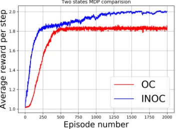
Figure 1: Simple deterministic MDP of two states and two actions
Figure 2: Average reward for INOC reaches the maxima while that of OC is stuck in a plateau. Results averaged over 200 runs of 2000 episodes.
gradient,∇θe qπO(s0, o0), as opposed to usingµO(s, o). Note
that the effectiveness of the natural policy gradient has been demonstrated sufficiently in past work (Kakade 2001; Bag-nell and Schneider 2003; Degris, Pilarski, and Sutton 2012). We define a simple 2 state MDP as in Figure 1. The initial state distribution isd0(s1) = 0.8andd0(s2) = 0.2. The transitions are deterministic. The reward for self loops into
s1ands2are 1 and 2, respectively. The episode terminates
after 30 steps. We use an-greedy policy over options,πO. We consider a scenario with two options,o1ando2, each of
which has probability 0.9 for actionsa1anda2, respectively,
regardless of the state. This gives us options as abstractions over individual actions. We initialize the terminations,βo, and option value function,qπO(s, o)such that they are biased
towards the greedy action,a1, in states1via the selection of
optiono1. Specifically, we setβo1(s1) = 0.1andβo1(s2) =
0.1, this way the setup is biased towards higher probability ofµO(s1, o1). This presents the agent with the challenge
of learning the more optimal action of transitioning to state
s2, despite the higher probabilityµ(s1, o1)and the self loop
reward ofs1. We set the learning rate for the intra-option
policies,αθ, to be negligible as our goal is to demonstrate the efficacy of the natural termination gradient.
As can be seen from Figure 2, the natural option critic converges to the optimal value, by overcoming the plateau, for average reward much faster than the option critic. The option critic is initially stuck in the greedy self-loop action, this is due to the weighting byµO(s, o). Whereas the natural option critic begins learning early on and achieves the optimal average reward.
Four Rooms: The four rooms domain (Sutton, Precup,
Figure 3: Four rooms withαθ =αϑ = 0.0025,αη = 0.5,
αϕ = 0.75,λ= 0.5and critic LR 0.5, averaged over 350 runs
and Singh 1999) is a particularly favorable case for demon-strating the use of options. We use the same number of options, 4, as in previous work (Bacon, Harb, and Precup 2017). The result (Figure 3) indicates that natural option critic converges faster.
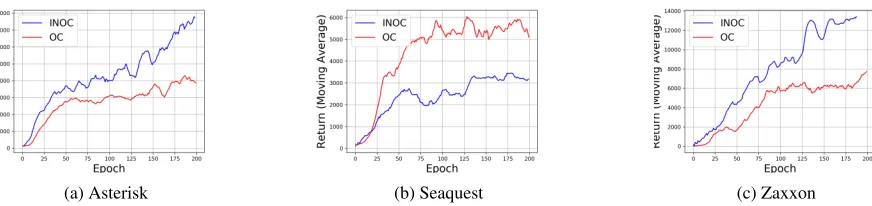
Arcade Learning Environment:
We compare natural option-critic with the option critic framework on the Arcade Learning Environment (Bellemare et al. 2013). To showcase the improvement over the option-critic architecture we use the same configuration for all the layers as in previous work (Bacon, Harb, and Precup 2017). Which in turn uses the same configuration for the first 3 convolutional layers of the network introduced by Mnih et al. (2013). The critic network was trained, similar to previous work (Bacon, Harb, and Precup 2017), using experience replay (Mnih et al. 2013) and RMSProp.
As in previous work (Bacon, Harb, and Precup 2017), we apply the regularizer prescribed by Mnih et al. (2016) to pe-nalize low entropy policies. We use an on-policy estimate of the policy over options,πO, which is used in the computa-tion of the natural gradient with respect to the terminacomputa-tion parameters.
We compare the two approaches, option critic and natu-ral option critic, by evaluating them for the gamesAsterisk, Seaquest,andZaxxon(Bacon, Harb, and Precup 2017). For comparison we run training over same number of frames per epoch as done by Bacon, Harb, and Precup (2017), running the same number of trial and use the same number of options: 8. We demonstrate the results in Figure 4. More impor-tantly, we use the same hyperparameters, for learning rates and entropy regularization, as in previous work to merit a fair comparison. We obtain improvements on the option-critic architecture (OC) for Asterisk and Zaxxon. We also note that we were unable to reproduce the results for Seaquest for op-tion critic, but having given the same set of hyperparameters we observe that option critic performs better. We explain the issue with termination updates, and it’s effect on the return, for Seaquest in the appendix.
(a) Asterisk (b) Seaquest (c) Zaxxon
Figure 4: Moving average of 10 returns for a single trial for Arcade learning Environment, with αθ = αϑ = 0.0025,
αη=αϕ= 0.75, andλ= 0.5
Discussion
We have introduced a natural gradient based approach for learning intra-option policies and terminations, within the option-critic framework, which is linear in the number of parameters. More importantly, we have furnished instructive proofs on deriving the Fisher information matrix over path manifolds and corresponding function approximations based approach while reducing mean squared errors. We have also introduced an algorithm that uses consistent estimates of the advantage functions and learn the natural gradient by learning coefficients of the corresponding linear function approxima-tors. The results showcase performance improvements on previous work. The proofs for finite horizon metrics are very similar to the ones provided by Bagnell and Schneider (2003). We also demonstrate the effectiveness of natural option critic in three distinct domains.
As discussed by Thomas (2014) we can obtain a truly unbiased estimate for our updates, but it may not be practical (Thomas 2014). The limitations that apply to the option-critic framework, except the use of vanilla gradient, apply. We use a block diagonal estimate of the Fisher information matrix. The complete Fisher information matrix for the option-critic framework over path manifolds is:
Gθ,ϑ=
Gθ h∂X∂θ∂X∂ϑi h∂X
∂ϑ ∂X
∂θi Gϑ
,
where Gθ andGϑ are the Fisher information matrices for intra-option path manifold and state-option transition man-ifold, respectively. The random variableXis the path vari-able over state-option-action tuples. The computation of the complete Fisher information matrix suffers and its inverse is expensive and needs a compatible function approximation based approach to obtain a natural gradient estimate with space complexity linear in number of parameters.
Although our approach has added benefits it is limited by fewer updates of the termination policy. Work is required to develop better estimates of the advantage functions. More experimental work, e.g. applications to other domains, can further help understand the efficacy of natural gradients in the context of the option-critic framework.
References
Amari, S. 1985. Differential-geometrical methods in statis-tics. InLecture Notes in Statistics 28. Springer-Verlag.
Amari, S.-I. 1998. Natural gradient works efficiently in learning.Neural Comput.10(2):251–276.
Amari, S.-i. 2016. Information Geometry and Its Applica-tions. Springer.
Bacon, P.-L.; Harb, J.; and Precup, D. 2017. The option-critic architecture. InAAAI.
Bagnell, J. A., and Schneider, J. 2003. Covariant policy search. IJCAI.
Bellemare, M. G.; Naddaf, Y.; Veness, J.; and Bowling, M. H. 2013. The arcade learning environment: An evaluation platform for general agents.J. Artif. Intell. Res.47:253–279.
Bhatnagar, S.; Sutton, R. S.; Ghavamzadeh, M.; and Lee, M. 2007. Incremental natural actor-critic algorithms. In Proceedings of the 20th International Conference on Neural Information Processing Systems, NIPS’07, 105–112. USA: Curran Associates Inc.
Bhatnagar, S.; Sutton, R. S.; Ghavamzadeh, M.; and Lee, M. 2009. Natural actor-critic algorithms. Automatica 45(11):2471–2482.
Degris, T.; Pilarski, P. M.; and Sutton, R. S. 2012. Model-free reinforcement learning with continuous action in practice.
DeGroot, M. 1970. Optimal Statistical Decisions. Wiley Classics Library. Wiley.
Desjardins, G.; Simonyan, K.; Pascanu, R.; et al. 2015. Natural neural networks. InAdvances in Neural Information Processing Systems, 2071–2079.
Dietterich, T. G. 2000. Hierarchical reinforcement learning with the maxq value function decomposition. J. Artif. Intell. Res.(JAIR)13(1):227–303.
Kakade, S. 2001. A natural policy gradient. In Dietterich, T. G.; Becker, S.; and Ghahramani, Z., eds.,Advances in Neu-ral Information Processing Systems 14 (NIPS 2001), 1531– 1538. MIT Press.
Konda, V. R., and Tsitsiklis, J. N. 2000. Actor-critic algo-rithms. NIPS’2000, 1008–1014.
Kurita, T. 1992. Iterative weighted least squares algorithms for neural networks classifiers.New Generation Computing 12:375–394.
Machado, M. C.; Bellemare, M. G.; and Bowling, M. 2017. A Laplacian framework for option discovery in reinforcement learning. In Precup, D., and Teh, Y. W., eds.,Proceedings of the 34th International Conference on Machine Learning, volume 70 ofProceedings of Machine Learning Research, 2295–2304. International Convention Centre, Sydney, Aus-tralia: PMLR.
Martens, J., and Grosse, R. B. 2015. Optimizing neural networks with kronecker-factored approximate curvature. In ICML.
Martens, J. 2010. Deep learning via hessian-free optimiza-tion. InProceedings of the 27th International Conference on International Conference on Machine Learning, ICML’10, 735–742. USA: Omnipress.
Mnih, V.; Kavukcuoglu, K.; Silver, D.; Graves, A.; Antonoglou, I.; Wierstra, D.; and Riedmiller, M. A. 2013. Playing atari with deep reinforcement learning. CoRR abs/1312.5602.
Mnih, V.; Badia, A. P.; Mirza, M.; Graves, A.; Lillicrap, T. P.; Harley, T.; Silver, D.; and Kavukcuoglu, K. 2016. Asynchronous methods for deep reinforcement learning. In ICML.
Morimura, T.; Uchibe, E.; and Kenji, D. 2005. Utilizing the natural gradient in temporal difference reinforcement learning with eligibility traces. 0–0.
Parr, R., and Russell, S. J. 1998. Reinforcement learning with hierarchies of machines. InAdvances in neural information processing systems, 1043–1049.
Pascanu, R., and Bengio, Y. 2013. Revisiting natural gradient for deep networks.
Peters, J., and Schaal, S. 2008. Natural actor-critic. Neuro-computing71:1180–1190.
Rao, C. R. 1945. Information and accuracy attainable in the estimation of statistical parameters. InBulletin of the Calcutta Mathematical Society. 81–91.
Roux, N. L.; Manzagol, P.; and Bengio, Y. 2008. Top-moumoute online natural gradient algorithm. In Platt, J. C.; Koller, D.; Singer, Y.; and Roweis, S. T., eds.,Advances in Neural Information Processing Systems 20. Curran Asso-ciates, Inc. 849–856.
Simsek, ¨O., and Barto, A. G. 2008. Skill characterization based on betweenness. InNIPS.
Sun, K., and Nielsen, F. 2017. Relative fisher information and natural gradient for learning large modular models. In ICML.
Sutton, R. S.; McAllester, D.; Singh, S.; and Mansour, Y. 1999. Policy gradient methods for reinforcement learning with function approximation. In Proceedings of the 12th International Conference on Neural Information Processing Systems, NIPS’99, 1057–1063.
Sutton, R. S.; Precup, D.; and Singh, S. P. 1999. Between mdps and semi-mdps: A framework for temporal abstraction in reinforcement learning.Artif. Intell.112:181–211.
Thomas, P. S., and Brunskill, E. 2017. Policy gradient meth-ods for reinforcement learning with function approximation and action-dependent baselines. CoRRabs/1706.06643. Thomas, P.; Silva, B. C.; Dann, C.; and Brunskill, E. 2016. Energetic natural gradient descent. In Balcan, M. F., and Weinberger, K. Q., eds.,Proceedings of The 33rd Interna-tional Conference on Machine Learning, volume 48 of Pro-ceedings of Machine Learning Research, 2887–2895. New York, New York, USA: PMLR.
Thomas, P. S.; Dann, C.; and Brunskill, E. 2018. Decoupling learning rules from representations. InICML.
Thomas, P. S. 2011. Policy gradient coagent networks. In Shawe-Taylor, J.; Zemel, R. S.; Bartlett, P. L.; Pereira, F.; and Weinberger, K. Q., eds.,Advances in Neural Information Processing Systems 24. Curran Associates, Inc. 1944–1952. Thomas, P. 2014. Bias in natural actor-critic algorithms. In ICML.