Multi-Dimensional Classification via kNN Feature Augmentation

(1)

The Thirty-Third AAAI Conference on Artificial Intelligence (AAAI-19)

Multi-Dimensional Classification via

k

NN Feature Augmentation

Bin-Bin Jia,

1,2,3

_{Min-Ling Zhang}

1,3,4,∗

1_{School of Computer Science and Engineering, Southeast University, Nanjing 210096, China}

2_{College of Electrical and Information Engineering, Lanzhou University of Technology, Lanzhou 730050, China} 3_{Key Laboratory of Computer Network and Information Integration (Southeast University), Ministry of Education, China}

4_{Collaborative Innovation Center of Wireless Communications Technology, China}

[email protected], [email protected]* (corresponding author)

Abstract

Multi-dimensional classification (MDC) deals with the prob-lem where one instance is associated with multiple class vari-ables, each of which specifies its class membership w.r.t. one specific class space. Existing approaches learn from MDC examples by focusing on modeling dependencies among class variables, while the potential usefulness of manipulat-ing feature space hasn’t been investigated. In this paper, a first attempt towards feature manipulation for MDC is pro-posed which enriches the original feature space withk NN-augmented features. Specifically, simple counting statistics on the class membership of neighboring MDC examples are used to generate augmented feature vector. In this way, dis-criminative information from class space is encoded into the feature space to help train the multi-dimensional classifica-tion model. To validate the effectiveness of the proposed feature augmentation techniques, extensive experiments over eleven benchmark data sets as well as four state-of-the-art MDC approaches are conducted. Experimental results clearly show that, compared to the original feature space, classifica-tion performance of existing MDC approaches can be signif-icantly improved by incorporatingkNN-augmented features.

Introduction

Multi-dimensional classification aims at modeling real-world objects with rich semantics, which assumes a number of class spaces to characterize the object’s semantics from different dimensions. Here, an MDC example is associated with multiple class variables with each of them specifying its class membership w.r.t. one specific class space. Specif-ically, the need of learning from MDC examples naturally arises in many scenarios (Theeramunkong and Lertnattee 2002; Rodr´ıguez et al. 2012; Borchani et al. 2013; Sagarna et al. 2014; Hern´andez-Gonz´alez, Inza, and Lozano 2015; Serafino et al. 2015). For example, the semantics of a natu-ral scene image can be characterized from theseason di-mension (with possible classesspring,summer,autumn, and

winter), and from thelandscapedimension (with possi-ble classesmountain,grassland,lake, etc.). For another ex-ample, the semantics of a piece of music can be character-ized from thegenredimension (with possible classesrock,

popular,classical, etc.), from theinstrumentdimension

(with possible classespiano,violin,guitar, etc.), and from the language dimension (with possible classes English,

Chinese,Spanish, etc.).

Formally, let X = Rd denote the d-dimensional input

(feature) space andY =C1×C2×· · ·×Cqdenote the output space which corresponds to the Cartesian product ofqclass spaces. Here, each class spaceCj (1 ≤j ≤q)consists of

Kjpossible classes, i.e.Cj ={cj1, c

j

2, . . . , c

j

Kj}. Given a set

of MDC training examplesD = {(xi,yi) | 1 ≤ i ≤ m}, wherexi = [xi1, xi2, . . . , xid]> ∈ X is a d-dimensional feature vector and yi = [yi1, yi2, . . . , yiq]> ∈ Y is the associated class vector with each component class variable

yij assuming one possible value inCj, the task of multi-dimensional classification is to learn a predictive function

f :X 7→ Y fromDwhich can assign a proper class vector

f(x)∈ Yfor unseen instancex.

To learn from MDC examples, an intuitive solution is to decompose the multi-dimensional classification problem into a number of independent multi-class classification prob-lems, one per class space. Nonetheless, dependencies among class spaces are ignored in this case which would impact the generalization performance of induced predictive model. Therefore, existing MDC approaches work by modeling dependencies among class variables from different dimen-sions in various ways, such as capturing pairwise inter-actions between class variables (Arias et al. 2016), spec-ifying chaining order over class variables (Zaragoza et al. 2011; Read, Martino, and Luengo 2014), assuming directed acyclic graph (DAG) structure over class variables (Bielza, Li, and Larrañaga 2011; Batal, Hong, and Hauskrecht 2013; Zhu, Liu, and Jiang 2016; Bolt and van der Gaag 2017; Benjumeda, Bielza, and Larrañaga 2018), and partitioning class variables into groups (Read, Bielza, and Larrañaga 2014), etc.

(2)

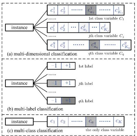
Figure 1: Relationships among multi-dimensional classifica-tion, multi-label classificaclassifica-tion, and multi-class classification.

discriminative information from class space is encoded into the feature space to facilitate subsequent induction of MDC predictive model. Extensive experiments clearly validate the effectiveness of KRAMin improving predictive performance of existing MDC approaches withkNN-augmented features. The rest of this paper is organized as follows. Firstly, re-lated works on multi-dimensional classification are briefly discussed. Secondly, technical details of the proposed ap-proach are introduced. Thirdly, experimental results of com-parative studies are reported. Finally, we conclude this paper.

Related Work

In multi-dimensional classification each instance is associ-ated with multiple class variables, whose most relassoci-ated learn-ing frameworks include traditional multi-class classification and multi-label classification (MLC) (Zhang and Zhou 2014; Gibaja and Ventura 2015).

As shown in Figure 1, MDC corresponds to a set of joint multi-class classification problems while MLC corresponds to a set of joint binary classification problems. Nonetheless, the major differences between MDC and MLC do not just lie in whether the joint problem to be solved is multi-class or binary class. Conceptually speaking, MDC usually assumes

heterogenoussemantic spaces where each class variable cor-responds to one possible class space, while MLC assumes

homogeneoussemantic space where each label specifies the relevancy of one concept in the class space. Formally speak-ing, MLC can be regarded as a degenerated version of MDC by restricting binary-valued class variable in each dimen-sion.

MDC can be decomposed into multiple traditional multi-class multi-classification problems, i.e. training an independent multi-class classifier w.r.t. each class space. However, this

intuitive strategy doesn’t consider possible dependencies among class spaces and may lead to suboptimal MDC solu-tion. Therefore, modeling dependencies among class spaces is one of the core goals when designing MDC learning ap-proaches.

Pairwise interactions between class spaces can be en-coded using a collection of base classifiers, where predic-tions from base classifiers are combined via Markov ran-dom field for subsequent multi-dimensional inference (Arias et al. 2016). Following the idea of classifier chain (CC) for MLC (Read et al. 2011), the MDC problem can be trans-formed into a chain of multi-class classification problems where the chaining order over class variables are specified in random manner (Read, Martino, and Luengo 2014) or de-terministic manner (Zaragoza et al. 2011).

Moreover, dependencies among class spaces can be ex-plicitly modeled with directed acyclic graph (DAG) with dif-ferent families of DAG structures (Bielza, Li, and Larra˜naga 2011; Batal, Hong, and Hauskrecht 2013; Zhu, Liu, and Jiang 2016; Bolt and van der Gaag 2017; Benjumeda, Bielza, and Larra˜naga 2018). Class powerset (CP) models dependencies by transforming the MDC problem into a sin-gle multi-class classification problem, where each possible combination of class variables y ∈ Y is treated as a new class in the transformed problem. In light of the huge class space (withQq

j=1Kj classes after CP transformation), it is helpful to partition MDC class variables into groups so as to expedite subsequent MDC model induction (Read, Bielza, and Larra˜naga 2014).

The K

RAM

Approach

Although modeling dependencies among class spaces plays a crucial role in learning from MDC examples, the impor-tance of manipulating feature space for model induction hasn’t been well studied for MDC researches. In this section, we present technical details of the KRAM approach which aims to improve the generalization ability of learned MDC models by enriching the original feature space with kNN techniques.

Following the same notations given in previous section, let D = {(xi,yi) | 1 ≤ i ≤ m} be the MDC train-ing set where yi = [yi1, yi2, . . . , yiq]> ∈ Y corresponds to the class vector associated withxi. For each instancex, let N(x) = {ir | 1 ≤ r ≤ k} denote the set of indices for theknearest neighbors ofxidentified inD. Then, the following counting statisticsδx

j = [δxj1, δjx2, . . . , δxjKj]

>_can

be defined for thej-th class space by considering the class membership of neighboring MDC examples:

δ_jax = X

ir∈N(x)

Jyirj =c

j

aK (1≤a≤Kj) (1)

Here,yir = [yir1, yir2, . . . , yirq]

>_{corresponds to the class}

vector of the neighboring MDC example xir for x. The

predicateJπKreturns 1 if πholds and 0 otherwise.

There-fore,δx

ja records the number ofx’s neighboring MDC ex-amples which has class value ofcj_a in thej-th class space. According to Eq.(1), it is easy to verify thatPKj

(3)

Table 1: The pseudo-code of KRAM.

Inputs:

D: MDC training set{(xi,yi)|1≤i≤m}

k: number of nearest neighbors considered L: MDC training algorithm

x∗: unseen instance

Outputs:

y∗: predicted class vector forx∗

Process:

1: fori= 1tomdo

2: Identifyknearest neighbors ofxiinDand store their indices inN(xi);

3: forj= 1toqdo

4: fora= 1toKjdo

5: Calculateδxi

ja according to Eq.(1);

6: end for

7: Setδxi

j = [δ

xi

j1, δ

xi

j2, . . . , δ

xi

jKj]

>_;

8: end for

9: Set∆xi =

δxi 1 ,δ

xi

2 , . . . ,δxqi

;

10: end for

11: Form the transformed MDC training setDe={(x_ei,yi)|

1≤i≤m}according to Eq.(3);

12: Induce MDC predictive function f based on D:e f ←_[ L(De);

13: Identifyknearest neighbors ofx∗inDand store their indices inN(x∗);

14: Generate augmented instance x˜∗ = [x∗,∆x∗] with

∆x∗being calculated according to Eq.(2) and Eq.(1);

15: Returny∗=f( ˜x∗).

Therefore, a total ofqcounting statisticsδx_j (1≤j ≤q)

each containingKjelements can be generated by traversing all class spaces. By concatenating all counting statistics, an augmented feature vector∆xforxis defined as follows:

∆x=

δx₁,δ₂x, . . . ,δ_qx

(2)

Then, the original MDC training setDis transformed into:

e

D={( ˜xi,yi)|1≤i≤m}, where ˜xi= [xi,∆xi] (3)

Here, each instancex˜i belongs to the augmented feature space Xe which is the Cartesian product betweenX and a (Pq

j=1Kj)-dimensional feature space. Thereafter, an MDC predictive functionf :X 7→ Ye can be induced fromDe by applying any MDC training algorithmL, i.e. f ←_[ L(De). For unseen instancex∗, its class vectory∗can be predicted by feeding the augmented instancex˜∗intof.

In summary, Table 1 presents the complete procedure of KRAM. Firstly, the original feature space is enriched bykNN feature augmentation based on simple counting statistics de-rived from neighboring MDC examples (steps 1-10). Af-ter that, an MDC predictive function is induced by learning from the transformed MDC training set (steps 11-12). Fi-nally, the class vector for unseen instance is predicted based on the augmented features as well (steps 13-15).

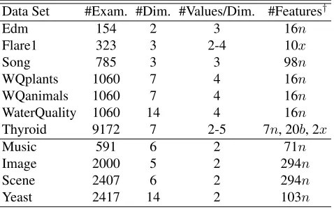
Table 2: Characteristics of the experimental data sets.

Data Set #Exam. #Dim. #Values/Dim. #Features†

Edm 154 2 3 16n

Flare1 323 3 2-4 10x

Song 785 3 3 98n

WQplants 1060 7 4 16n

WQanimals 1060 7 4 16n

WaterQuality 1060 14 4 16n

Thyroid 9172 7 2-5 7n, 20b, 2x

Music 591 6 2 71n

Image 2000 5 2 294n

Scene 2407 6 2 294n

Yeast 2417 14 2 103n

† _n_,_b_and_x_{denote numeric, binary, and nominal features}

respectively.

It is worth noting that the proposed KRAM approach should be regarded as a meta-strategy to learn from MDC examples, where any off-the-shelf MDC training algorithm L can be utilized to instantiate KRAM. Moreover, the

kNN-based techniques proposed in this paper only repre-sent as a first attempt towards MDC feature augmentation, which is not meant to be the best possible practice among other feasible choices. Nevertheless, experimental studies reported in the next section clearly validate the effectiveness of KRAM in improving the generalization performance of multi-dimensional classification.

Experiments

Experimental Setup

Data Sets To evaluate the effectiveness of KRAM in im-proving the generalization performance of MDC predictive model, a number of MDC data sets have been employed for experimental studies. Table 2 summarizes characteristics of the experimental data sets, including number of examples

(#Exam.),number of class spaces(#Dim.),number of class values per class space(#Values/Dim.), andnumber of fea-tures(#Features).

The first seven data sets in Table 2 are collected from dif-ferent real-world MDC tasks:1

• Edmdeals with the task of predicting control operations during electrical discharge machining process (Karaliˇc and Bratko 1997), where the 2 class spaces correspond to two controlling parameters gap and flow.

• Flare1deals with the task of predicting the number of times certain types of solar flare occurred within 24 hours period (Dheeru and Karra Taniskidou 2017), where the 3 class spaces correspond to common, moderate, and severe solar flares.

1

(4)

Table 3: Experimental results (mean±std. deviation) of each MDC approach and its KRAMcounterpart in terms ofhamming score. In addition,•/◦indicates whether the KRAMcounterpart is significantly superior/inferior to the MDC approach on each data set (pairwiset-test at 0.05 significance level).

(a) Multi-class classifier: SVM

Data Set BR KRAM-BR ECC KRAM-ECC ECP KRAM-ECP ESC KRAM-ESC

Edm .689±.070 .734±.083• .695±.065 .769±.087• .721±.082 .763±.107• .698±.089 .751±.102•

Flare1 .922±.034 .922±.033 .922±.034 .922±.034 .921±.036 .922±.034 .923±.033 .923±.036

Song .793±.023 .787±.023◦ .790±.024 .788±.026 .786±.029 .781±.028 .790±.029 .788±.029

WQplants .657±.016 .664±.013 .654±.016 .663±.014• .647±.015 .585±.027◦ .651±.017 .664±.016•

WQanimals .630±.014 .635±.012• .630±.014 .637±.014• .629±.013 .556±.014◦ .631±.014 .635±.014

WaterQuality .644±.013 .646±.010 .643±.013 .644±.013 .628±.015 .557±.010◦ .641±.013 .636±.013

Thyroid .965±.002 .969±.003• .965±.002 .969±.003• .965±.002 .968±.002• .965±.002 .969±.002•

Music .808±.023 .818±.022• .814±.025 .810±.022 .799±.032 .802±.025 .813±.028 .809±.029

Image .828±.010 .841±.011• .831±.012 .844±.012• .832±.012 .842±.009• .838±.009 .844±.015

Scene .895±.009 .918±.008• .905±.011 .921±.008• .914±.009 .925±.008• .910±.011 .923±.008•

Yeast .801±.006 .811±.007• .797±.007 .808±.007• .795±.007 .795±.007 .802±.006 .808±.008•

(b) Multi-class classifier: NB

Edm .677±.096 .680±.088 .690±.084 .674±.097 .731±.062 .722±.089 .674±.095 .674±.101

Flare1 .886±.061 .872±.051 .883±.059 .875±.053 .908±.045 .903±.046 .896±.059 .892±.053

Song .626±.038 .629±.034 .621±.036 .623±.034 .674±.044 .684±.042 .646±.031 .666±.037•

WQplants .397±.028 .506±.033• .353±.033 .494±.038• .607±.015 .647±.019• .442±.034 .549±.031•

WQanimals .381±.021 .419±.019• .377±.024 .416±.020• .590±.020 .625±.017• .577±.022 .598±.013•

WaterQuality .389±.017 .488±.022• .360±.020 .487±.021• .599±.018 .597±.018 .609±.017 .609±.017

Thyroid .926±.005 .925±.003 .926±.007 .929±.004 .966±.003 .963±.003◦ .958±.004 .952±.006◦

Music .743±.018 .761±.023• .745±.020 .761±.023• .770±.029 .784±.019• .738±.023 .764±.030•

Image .573±.016 .586±.018• .576±.014 .587±.014• .746±.012 .754±.011• .593±.017 .608±.015•

Scene .763±.009 .777±.009• .767±.010 .780±.010• .867±.011 .875±.013• .866±.010 .868±.013

Yeast .699±.010 .695±.014 .696±.009 .698±.013 .773±.011 .787±.008• .716±.006 .743±.006•

• Songdeals with the task of predicting properties of songs which are collected and annotated by ourselves, where the 3 class spaces correspond to the emotion, genre and sce-narios of one song.

• Water Qualitydeals with the task of predicting plant and animal species in Slovenian rivers (Dˇzeroski, Demˇsar, and Grbovi´c 2000), where the 14 class spaces correspond to relative representation of different species. By focusing on the 7 class spaces on plant or the 7 class spaces on animal, we have theWQplantsandWQanimalsdata sets respectively (Kocev et al. 2007).

• Thyroiddeals with the task of estimating types of thy-roid problems based on patient information (Dheeru and Karra Taniskidou 2017), where the 7 class spaces corre-spond to diagnosis of seven different conditions.

The last four data sets in Table 2 are collected from benchmark multi-label learning tasks including audio clas-sification:Music(Read, Bielza, and Larra˜naga 2014), im-age classification:Image,Scene(Zhang and Zhou 2007; Boutell et al. 2004), and gene functional analysis:Yeast

(Elisseeff and Weston 2002). Here, each class space

cor-responds to a binary-valued class variable which specifies whether one concept is relevant to the example or not.

Evaluation Metrics Let S = {(xi,yi) | 1 ≤ i ≤

p} be the test set with p MDC examples, where yi =

[yi1, yi2, . . . , yiq]> ∈ Y is the class vector associated with

xi. Furthermore, letf : X 7→ Y be the induced MDC pre-dictive function whereyî =f(xi) = [ˆyi1,yî2, . . . ,yîq]>is the predicted class vector forxi.

For each MDC test example (xi,yi), let r(i) =

Pq

j=1Jyij = ˆyijK denote the number of class spaces on

which f makes correct classification. Then, the following three metrics are utilized in this paper to measure the gener-alization performance of MDC approaches:

• Hamming Score:

HScoreS(f) = 1

p

p X

i=1 1

q·r

(i)

(5)

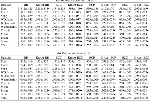
Table 4: Experimental results (mean±std. deviation) of each MDC approach and its KRAMcounterpart in terms ofexact match. In addition,•/◦indicates whether the KRAMcounterpart is significantly superior/inferior to the MDC approach on each data set (pairwiset-test at 0.05 significance level).

Edm .442±.125 .521±.141• .454±.123 .598±.169• .559±.136 .612±.170 .513±.142 .592±.165•

Flare1 .821±.073 .818±.072 .817±.078 .818±.073 .817±.078 .821±.073 .821±.073 .821±.073

Song .479±.059 .476±.050 .481±.057 .476±.051 .484±.054 .467±.059 .481±.062 .480±.057

WQplants .097±.033 .099±.034 .093±.037 .105±.037 .093±.028 .067±.029◦ .093±.037 .099±.032

WQanimals .058±.022 .063±.014 .061±.023 .064±.010 .065±.018 .029±.011◦ .064±.024 .059±.014

WaterQuality .007±.008 .008±.007 .006±.008 .009±.006 .001±.003 .004±.005 .006±.008 .010±.005

Thyroid .773±.015 .800±.018• .772±.014 .800±.016• .773±.014 .802±.015• .771±.014 .801±.015•

Music .272±.075 .331±.082• .346±.079 .343±.078 .343±.076 .341±.073 .350±.078 .345±.084

Image .394±.028 .459±.033• .479±.033 .522±.036• .513±.024 .540±.024• .499±.025 .529±.038•

Scene .530±.035 .651±.038• .649±.035 .708±.026• .700±.029 .731±.029• .665±.041 .725±.027•

Yeast .151±.017 .199±.015• .207±.014 .252±.014• .252±.012 .262±.018 .237±.017 .263±.019•

Edm .432±.166 .445±.153 .451±.145 .438±.162 .554±.112 .548±.120 .432±.166 .438±.162

Flare1 .774±.099 .756±.095 .774±.087 .771±.088 .790±.081 .777±.084 .780±.093 .768±.086

Song .238±.054 .224±.050 .228±.036 .219±.043 .311±.053 .317±.051 .274±.047 .304±.054•

WQplants .001±.003 .036±.026• .001±.003 .035±.018• .034±.021 .067±.038• .001±.003 .040±.025•

WQanimals .004±.009 .008±.010 .007±.008 .006±.007 .020±.014 .042±.016• .024±.018 .026±.023

WaterQuality .000±.000 .000±.000 .000±.000 .000±.000 .008±.009 .004±.007◦ .002±.004 .002±.004

Thyroid .580±.027 .575±.015 .593±.026 .592±.022 .793±.017 .768±.015◦ .738±.022 .703±.036◦

Music .206±.043 .218±.058 .230±.058 .221±.065 .249±.078 .281±.073• .210±.070 .242±.089•

Image .069±.016 .074±.021• .069±.019 .074±.020• .285±.022 .302±.022• .069±.021 .074±.021

Scene .177±.023 .198±.022• .181±.024 .200±.021• .550±.030 .575±.040• .541±.024 .528±.046

Yeast .095±.018 .115±.018• .102±.016 .125±.024• .203±.018 .240±.024• .110±.014 .154±.015•

• Exact Match:

EMatchS(f) = 1

p

p X

i=1 Jr

(i)₌_q K

The exact match measures the proportion of test examples on which the MDC predictor makes correct classification over all class spaces. Conceptually, exact match serves as a strict metric whose value might be rather low for MDC tasks with large number of class spaces.

• Sub-Exact Match:

SEMatchS(f) = 1

p

p X

i=1 Jr

(i)

≥q−1_K

The sub-exact match corresponds to a relaxed version of exact match, which measures the proportion of test ex-amples on which the MDC predictor makes at most one incorrect classification over all class spaces.

Comparing Approaches KRAM is a meta-strategy to learn from MDC examples, which can be coupled with any off-the-shelf MDC learning algorithm (i.e. L in Table 1)

to improve its generalization performance. In this paper, four well-established MDC approaches (Read, Bielza, and Larra˜naga 2014) are used to instantiate KRAM:

• Binary Relevance(BR): This approach decomposes the multi-dimensional classification problem into a number of independent multi-class classification problems, one per class space.

• Ensembles of Classifier Chains (ECC): This approach transforms the multi-dimensional classification problem into a chain of multi-class classification problems, where subsequent classifiers in the chain are built by treating predictions of preceding ones as extra features. Specifi-cally, an ensemble of classifier chains are built with dif-ferent random chaining orders.

(6)

Table 5: Experimental results (mean±std. deviation) of each MDC approach and its KRAMcounterpart in terms ofsub-exact match. In addition,•/◦indicates whether the KRAMcounterpart is significantly superior/inferior to the MDC approach on each data set (pairwiset-test at 0.05 significance level).

Edm .935±.061 .947±.076 .935±.069 .940±.058 .883±.074 .915±.075 .883±.074 .909±.070

Flare1 .947±.039 .951±.036 .951±.036 .951±.036 .947±.039 .947±.039 .951±.036 .951±.042

Song .903±.033 .888±.046 .891±.036 .891±.047 .878±.040 .877±.040 .892±.038 .885±.048

WQplants .287±.055 .300±.042 .283±.049 .295±.044 .281±.049 .187±.040◦ .282±.049 .294±.045

WQanimals .229±.034 .232±.030 .229±.032 .241±.040 .230±.032 .151±.030◦ .232±.032 .241±.032

WaterQuality .051±.024 .053±.017 .050±.023 .048±.018 .035±.018 .019±.016 .046±.022 .049±.024

Thyroid .982±.004 .983±.004 .981±.004 .982±.004 .981±.005 .979±.003◦ .982±.004 .981±.004

Music .674±.067 .682±.054 .676±.064 .677±.051 .640±.064 .659±.066 .662±.075 .672±.063

Image .782±.031 .783±.027 .730±.033 .745±.031 .710±.036 .727±.029• .738±.032 .740±.036

Scene .855±.018 .867±.020 .796±.030 .825±.020• .796±.028 .825±.018• .799±.032 .823±.024•

Yeast .269±.029 .307±.020• .288±.023 .316±.022• .304±.020 .317±.018 .310±.030 .324±.027•

Edm .922±.074 .916±.060 .929±.064 .909±.062 .909±.047 .896±.081 .915±.063 .909±.062

Flare1 .910±.066 .895±.055 .904±.073 .889±.060 .941±.057 .938±.057 .929±.064 .926±.060

Song .678±.071 .695±.068 .671±.068 .683±.066 .733±.079 .749±.080 .692±.066 .719±.067•

WQplants .018±.012 .113±.040• .013±.010 .123±.037• .175±.043 .258±.056• .042±.019 .133±.031•

WQanimals .041±.016 .049±.019 .039±.016 .049±.015• .143±.054 .221±.049• .139±.050 .167±.045

WaterQuality .000±.000 .003±.005 .000±.000 .001±.003 .032±.024 .033±.020 .023±.013 .025±.017

Thyroid .916±.011 .912±.009 .906±.020 .922±.008• .974±.005 .973±.005 .970±.007 .966±.006

Music .552±.057 .591±.050• .557±.051 .603±.048• .591±.071 .617±.053 .524±.039 .581±.082•

Image .255±.028 .279±.034• .261±.028 .283±.033• .597±.034 .612±.033• .289±.032 .315±.029•

Scene .561±.021 .591±.026• .569±.027 .595±.031• .693±.031 .713±.036• .703±.031 .733±.038•

Yeast .149±.020 .182±.027• .163±.020 .193±.027• .258±.022 .293±.022• .167±.019 .217±.022•

• Ensembles of Super Class classifiers (ESC): This ap-proach works by partitioning the MDC class variables into groups of super-classes, where conditional dependencies among class variables are used to fulfill the partition pro-cess. Specifically, an ensemble of super-class models are built by randomly sampling the MDC training set.

Following (Read, Bielza, and Larra˜naga 2014), a random cut of 67% examples from the original MDC training set is used to generate the base MDC model and the number of base classifiers is set to be 10 for ensemble approaches ECC, ECP and ESC. Furthermore, predictions of base MDC models are combined via majority voting.

For each MDC approachA(A ∈{BR, ECC, ECP, ESC}), we use KRAM-Ato denote the instantiation of KRAMwith A. In this paper, support vector machine (SVM) (Chang and Lin 2011) and Na¨ıve Bayes (NB) are used as the multi-class classifier to implement each MDC approach. Specifically, Libsvm with linear kernel and NB with Gaussian pdf for continuous feature are used. As shown in Table 1, the only parameterk(number of nearest neighbors considered) is set to be 8 for KRAM.

To show the effectiveness of KRAM, we aim to compare

the performance of KRAM-Aagainst A. On each data set, ten-fold cross-validation is performed where the mean met-ric value as well as standard deviation are recorded for the comparing approaches.

Experimental Results

Tables 3 to 5 report the detailed experimental results of each MDC approach and its KRAMcounterpart in terms of ham-ming score,exact match, andsub-exact matchrespectively. For each data set and multi-class classifier (SVM or NB), pairwise t-test based on ten-fold cross-validation (at 0.05 significance level) is conducted to show whether the perfor-mance of KRAMcounterpart is significantly different to the MDC approach. Accordingly, Table 6 summarizes the re-sulting win/tie/loss counts over 11 data sets and 3 evaluation metrics.

Based on the reported experimental results, it is interest-ing to observe that:

(7)

Table 6: Win/tie/loss counts of pairwiset-test (at 0.05 significance level) between each MDC approach and its KRAM counter-part in terms ofhamming score(HScore),exact match(EMatch), andsub-exact match(SEMatch).

multi-class classifier: SVM multi-class classifier: NB

HScore EMatch SEMatch HScore EMatch SEMatch In Total

KRAM-BR against BR 7/3/1 6/5/0 1/10/0 6/5/0 4/7/0 5/6/0 29/36/1

KRAM-ECC against ECC 7/4/0 5/6/0 2/9/0 6/5/0 4/7/0 7/4/0 31/35/0

KRAM-ECP against ECP 4/4/3 3/6/2 2/6/3 6/4/1 6/3/2 5/6/0 26/29/11

KRAM-ESC against ESC 5/6/0 5/6/0 2/9/0 6/4/1 4/6/1 6/5/0 28/36/2

(a)hamming score (b)exact match (c)sub-exact match

Figure 2: Performance of KRAM-BR changes askranges from 5 to 10 in terms of each evaluation metric.

configurations.

• BR learns from MDC examples by independent decompo-sition, where dependencies among class spaces have not been considered in this approach. The prominent advan-tage of KRAM-BR over BR (with only one loss on HScore with SVM) indicates that the kNN-augmented features generated by KRAMdo bring helpful discriminative infor-mation in feature space. Specifically, those discriminative information brought into feature space can be regarded as a potential source for dependency modeling when learn-ing the mapplearn-ing from feature space to output space.

• Both ECC and ESC learn from MDC examples by con-sidering dependencies among class spaces, which are fulfilled by assuming random chaining order over class spaces or partitioning the class spaces into groups. It is impressive to notice that for MDC approaches with inherent dependency modeling mechanism, KRAM can also help improve their generalization ability significantly withkNN-augmented features.

• ECP learns from MDC examples by modeling full-order dependencies, where all possible combinations of class spaces (i.e. class powerset) have been considered in the learning process. ECP generally benefits from the kNN augmented features, while there are 11 cases where the performance of KRAM-ECP is inferior to ECP. Most of the under-performing cases (8 out of 11) for KRAM-ECP occur forWaterQuality(including its two divisions WQ-plantsandWQanimals), where the possible number of CP combinations is high (i.e.414).

As shown in Table 1, the only parameter to be set for KRAMisk, which is the number of nearest neighbors

con-sidered for generating kNN-augmented features. Figure 2 illustrates how the performance of KRAM (with MDC ap-proach BR) changes as kincreases from 5 to 10. In terms of each evaluation metric, KRAMachieves relatively stable performance with varying values ofk. Parameter insensitiv-ity is a desirable property for practical use of KRAM, and the value ofkis fixed to be 8 in this paper.

Conclusion

The major contributions of our work are two-fold: 1) A new strategy aiming at manipulating feature space for multi-dimensional classification is proposed, which suggests an al-ternative solution to learn from MDC examples; 2) A simple yet effective approach based onkNN-augmented features is designed to justify the proposed strategy, whose effective-ness is thoroughly validated based on extensive comparative studies. In the future, it is interesting to explore other ways for MDC feature space manipulation. Furthermore, design-ing feature augmentation techniques customized for specific MDC approach is also worth further investigation.

Acknowledgement

(8)

References

Arias, J.; Gamez, J. A.; Nielsen, T. D.; and Puerta, J. M. 2016. A scalable pairwise class interaction framework for multidimensional classification. International Journal of Approximate Reasoning68:194–210.

Batal, I.; Hong, C.; and Hauskrecht, M. 2013. An effi-cient probabilistic framework for multi-dimensional classifi-cation. InProceedings of the 22nd ACM International Con-ference on Information & Knowledge Management, 2417– 2422.

Benjumeda, M.; Bielza, C.; and Larra˜naga, P. 2018. Tractability of most probable explanations in multidimen-sional bayesian network classifiers.International Journal of Approximate Reasoning93:74–87.

Bielza, C.; Li, G.; and Larra˜naga, P. 2011. Multi-dimensional classification with bayesian networks. Inter-national Journal of Approximate Reasoning52(6):705–727. Bolt, J. H., and van der Gaag, L. C. 2017. Balanced sensitiv-ity functions for tuning multi-dimensional bayesian network classifiers.International Journal of Approximate Reasoning

80:361–376.

Borchani, H.; Bielza, C.; Toro, C.; and Larra˜naga, P. 2013. Predicting human immunodeficiency virus inhibitors using multi-dimensional bayesian network classifiers. Artificial Intelligence in Medicine57(3):219–229.

Boutell, M. R.; Luo, J.; Shen, X.; and Brown, C. M. 2004. Learning multi-label scene classification. Pattern Recogni-tion37(9):1757–1771.

Chang, C.-C., and Lin, C.-J. 2011. LIBSVM: A library for support vector machines. ACM Transactions on Intelligent Systems and Technology2:27:1–27:27. Software available at http://www.csie.ntu.edu.tw/∼_{cjlin/libsvm.}

Dheeru, D., and Karra Taniskidou, E. 2017. UCI machine learning repository. http://archive.ics.uci.edu/ml.

Dˇzeroski, S.; Demˇsar, D.; and Grbovi´c, J. 2000. Predicting chemical parameters of river water quality from bioindicator data.Applied Intelligence13(1):7–17.

Elisseeff, A., and Weston, J. 2002. A kernel method for multi-labelled classification. InAdvances in Neural Infor-mation Processing Systems, 681–687.

Gibaja, E., and Ventura, S. 2015. A tutorial on multilabel learning.ACM Computing Surveys47(3):Article 52. Hern´andez-Gonz´alez, J.; Inza, I.; and Lozano, J. A. 2015. Multidimensional learning from crowds: Usefulness and ap-plication of expertise detection.International Journal of In-telligent Systems30(3):326–354.

Karaliˇc, A., and Bratko, I. 1997. First order regression.

Machine Learning26(2-3):147–176.

Kocev, D.; Vens, C.; Struyf, J.; and Dˇzeroski, S. 2007. En-sembles of multi-objective decision trees. InLecture Notes in Computer Science 4701. Berlin: Springer. 624–631. Ma, Z., and Chen, S. 2018. Multi-dimensional classification via a metric approach.Neurocomputing275:1121–1131. Read, J.; Pfahringer, B.; Holmes, G.; and Frank, E. 2011.

Classifier chains for multi-label classification. Machine Learning85(3):333–359.

Read, J.; Bielza, C.; and Larra˜naga, P. 2014. Multi-dimensional classification with super-classes. IEEE Trans-actions on Knowledge and Data Engineering 26(7):1720– 1733.

Read, J.; Martino, L.; and Luengo, D. 2014. Efficient monte carlo methods for multi-dimensional learning with classifier chains. Pattern Recognition47(3):1535–1546.

Rodr´ıguez, J. D.; P´erez, A.; Arteta, D.; Tejedor, D.; and Lozano, J. A. 2012. Using multidimensional bayesian net-work classifiers to assist the treatment of multiple sclerosis.

IEEE Transactions on Systems, Man, and Cybernetics Part C: Applications and Reviews42(6):1705–1715.

Sagarna, R.; Mendiburu, A.; Inza, I.; and Lozano, J. A. 2014. Assisting in search heuristics selection through multidimen-sional supervised classification: A case study on software testing.Information Sciences258:122–139.

Serafino, F.; Pio, G.; Ceci, M.; and Malerba, D. 2015. Hier-archical multidimensional classification of web documents with multiwebclass. InLecture Notes in Computer Science 9356. Berlin: Springer. 236–250.

Theeramunkong, T., and Lertnattee, V. 2002. Multi-dimensional text classification. InProceedings of the 19th International Conference on Computational Linguistics-Volume 1, 1–7. Association for Computational Linguistics. Zaragoza, J. H.; Sucar, L. E.; Morales, E. F.; Bielza, C.; and Larra˜naga, P. 2011. Bayesian chain classifiers for multi-dimensional classification. InProceedings of the 22nd In-ternational Joint Conference on Artificial Intelligence, vol-ume 11, 2192–2197.

Zhang, M.-L., and Zhou, Z.-H. 2007. ML-KNN: A lazy learning approach to multi-label learning. Pattern Recogni-tion40(7):2038–2048.

Zhang, M.-L., and Zhou, Z.-H. 2014. A review on multi-label learning algorithms.IEEE Transactions on Knowledge and Data Engineering26(8):1819–1837.

Zhu, M.; Liu, S.; and Jiang, J. 2016. A hybrid method for learning multi-dimensional bayesian network classifiers based on an optimization model. Applied Intelligence