The Thirty-Third AAAI Conference on Artificial Intelligence (AAAI-19)
Multi-Source Neural Variational Inference
Richard Kurle
Department of Informatics Technical University of Munich,
Data:Lab, Volkswagen Group 80805 Munich, Germany
Stephan G ¨unnemann
Department of Informatics Technical University of Munich
Patrick van der Smagt
Data:Lab, Volkswagen Group 80805 Munich, Germany
Abstract
Learning from multiple sources of information is an impor-tant problem in machine-learning research. The key chal-lenges are learning representations and formulating inference methods that take into account the complementarity and re-dundancy of various information sources. In this paper we formulate a variational autoencoder based multi-source learn-ing framework in which each encoder is conditioned on a dif-ferent information source. This allows us to relate the sources via the shared latent variables by computing divergence mea-sures between individual source’s posterior approximations. We explore a variety of options to learn these encoders and to integrate the beliefs they compute into a consistent posterior approximation. We visualise learned beliefs on a toy dataset and evaluate our methods for learning shared representations and structured output prediction, showing trade-offs of learn-ing separate encoders for each information source. Further-more, we demonstrate how conflict detection and redundancy can increase robustness of inference in a multi-source setting.
1
Introduction
An essential feature of most living organisms is the ability to process, relate, and integrate information coming from a vast number of sensors and eventually from memories and pre-dictions (Stein and Meredith 1993). While integrating infor-mation from complementary sources enables a coherent and unified description of the environment, redundant sources are beneficial for reducing uncertainty and ambiguity. Fur-thermore, when sources provide conflicting information, it can be inferred that some sources must be unreliable.
Replicating this feature is an important goal of multi-modal machine learning (Baltruˇsaitis, Ahuja, and Morency 2017). Learning joint representations of multiple modalities has been attempted using various methods, including neural networks (Ngiam et al. 2011), probabilistic graphical models (Srivastava and Salakhutdinov 2014), and canonical correla-tion analysis (Andrew et al. 2013). These methods focus on learning joint representations and multimodal sensor fusion. However, it is challenging to relate information extracted from different modalities. In this work, we aim at learning probabilistic representations that can be related to each other by statistical divergence measures as well as translated from
Copyright c2019, Association for the Advancement of Artificial Intelligence (www.aaai.org). All rights reserved.
one modality to another. We make no assumptions about the nature of the data (i.e. multimodal or multi-view) and therefore adopt a more general problem formulation, namely learning from multipleinformation sources.
Probabilistic graphical models are a common choice to address the difficulties of learning from multiple sources by modelling relationships between information sources— i.e., observed random variables—via unobserved, random variables. Inferring the hidden variables is usually only tractable for simple linear models. For nonlinear models, one has to resort to approximate Bayesian methods. The variational autoencoder (VAE) (Kingma and Welling 2013; Rezende, Mohamed, and Wierstra 2014) is one such method, combining neural networks and variational inference for latent-variable models (LVM).
We build on the VAE framework, jointly learning the generative and inference models from multiple information sources. In contrast to the VAE, we encapsulate individual inference models into separate “modules”. As a result, we obtain multiple posterior approximations, each informed by a different source. These posteriors represent the belief over the same latent variables of the LVM, conditioned on the available information in the respective source.
Modelling beliefs individually—but coupled by the gen-erative model—enables computing meaningful quantities such as measures of surprise, redundancy, or conflict be-tween beliefs. Exploiting these measures can in turn increase the robustness of the inference models. Furthermore, we ex-plore different methods to integrate arbitrary subsets of these beliefs, to approximate the posterior for the respective sub-set of observations. We essentially modularise neural vari-ational inference in the sense that information sources and their associated encoders can be flexibly interchanged and combined after training.
2
Background—Neural variational inference
Consider a datasetX = {x(n)}N
n=1of N i.i.d. samples of
some random variablexand the following generative model:
pθ(x(n)) = Z
pθ(x(n)|z(n))p(z(n))dz(n),
autoen-coder (Kingma and Welling 2013; Rezende, Mohamed, and Wierstra 2014) is an approximate inference method that en-ables learning the parameters of this model by optimising an evidence lower bound (ELBO) to the log marginal like-lihood. A second neural network with parametersφdefines the parameters of an approximationqφ(z|x)of the poste-rior distribution. Since the computational cost of inference for each data point is shared by using a recognition model, some authors refer to this form of inference as amortised or neural variational inference (Gershman and Goodman 2014; Mnih and Gregor 2014).
The importance weighted autoencoder (Burda, Grosse, and Salakhutdinov 2015) (IWAE) generalises the VAE by using a multi-sample importance weighting estimate of the log-likelihood. The IWAE ELBO is given as:
lnpθ(x(n))≥Ez1:(nK)∼qφ(z(n)|x(n)) h
ln 1 K
K X
k=1
wk(n)i,
whereKis the number of importance samples, andwk(n)are the importance weights:
w(kn)=pθ(x
(n)|z(n)
k )p(z
(n)
k ) qφ(z
(n)
k |x(n)) .
Besides achieving a tighter lower bound, the IWAE was mo-tivated by noticing that a multi-sample estimate does not re-quire all samples from the variational distribution to have a high posterior probability. This enables the training of a generative model using samples from a variational distribu-tion with higher uncertainty. Importantly, this distribudistribu-tion need not be the posterior of all observations in the gener-ative model. It can be a good enough proposal distribution, i.e. the belief from a partially-informed source.
3
Multi-source neural variational inference
We are interested in datasets consisting of tuples{x(n) =
(x(1n), . . . , x(Mn))}N
n=1, we usem ∈ {1, . . . , M}to denote
the index of the source. Each observationx(mn)∈RDm may be embedded in a different space but is assumed to be gen-erated from the same latent statez(n). Therefore, eachx(n)
m
corresponds to a different, potentially limited source of in-formation about the underlying statez(n). From now on we
will refer toxmin the generative model as observations and
the samexmin the inference model as information sources.
We model each observationxmin the generative model
with a distinct set of parametersθm, although some param-eters could be shared. The likelihood function is given as:
pθ(x(n)|z(n)) = M Y
m=1
pθm x
(n)
m |z
(n) .
For inference, the VAE conditions on all observable data x(n). However, one can condition (amortize) the
approximate posterior distribution on any set of infor-mation sources. In this paper we limit ourselves to x(Sn), S⊂ {1, . . . , M}. An approximate posterior
distribu-tionqφS(z(n)|x(Sn))may then be interpreted as the belief of
the respective information sources about the latent variables, underlying the generative process.
In contrast to the VAE, we want to calculate the be-liefs from differentinformation sources individually, com-pare them, and eventually integrate them. In the following, we address each of these desiderata.
3.1
Learning individual beliefs
In order to learn individual inference models as in Fig. 1a, we propose an average ofM ELBOs, one for each informa-tion source and its respective inference model. The resulting objective is an ELBO to the log marginal likelihood itself and referred to asL(ind):
L(ind)=:
M X
m=1
πmEz(n)
1:K∼qφm z(n)|x(mn)
h ln 1
K K X
k=1
w(m,kn)i,
(1) with
wm,k(n) = pθ x
(n)|z(n)
k
p z(kn)
qφm z
(n)
k |x
(n)
m .
The indicesn,mandk refer to the data sample, informa-tion source, and importance sample index. The factorsπm
are the weights of the ELBOs, satisfying0 ≤πm≤1and PM
m=1πm= 1. Although theπmcould be inferred, we set
πm = 1/M, ∀m. This ensures that all parametersφm are
optimised individually to their best possible extent instead of down-weighting less informative sources.
Since we are dealing with partially-informed encoders
qφm(z(n)|x(n)
m )instead ofqφ(z(n)|x(n)), the beliefs can be
more uncertain than the posterior of all observationsx. This in turn degrades the generative model, as it requires samples from the posterior distribution. We found that the generative model becomes biased towards generating averaged samples rather than samples from a diverse, multimodal distribution. This issue arises in VAE-based objectives, irrespective of the complexity of the variational family, because each Monte-Carlo sample of latent variables must predict all observa-tions. To account for this, we propose to use importance sampling estimates of the log-likelihood (see Sec. 2). The importance weighting and sampling-importance-resampling can be seen as feedback from the observations, allowing to approximate the true posterior even with poorly informed beliefs.
3.2
Comparing beliefs
Encapsulating individual inferences has an appealing advan-tage compared to an uninterpretable, deterministic combina-tion within a neural network: Having obtained multiple be-liefs w.r.t. the same latent variables, each informed by a dis-tinct source, we can calculate meaningful quantities to relate the sources. Examples are measures of redundancy, surprise, or conflict. Here we focus on the latter.
z z . . . z
x1 x2 . . . xM
N N N
φ1 φ2 . . . φM
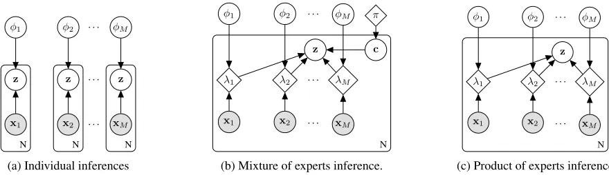
(a) Individual inferences
λ1 λ2 . . . λM
z c
π
x1 x2 . . . xM
N
φ1 φ2 . . . φM
(b) Mixture of experts inference.
λ1 λ2 . . . λM
z
x1 x2 . . . xM
N
φ1 φ2 . . . φM
(c) Product of experts inference
Figure 1: Graphical models of inference models. White circles denote hidden random variables, grey-shaded circles—observed random variables, diamonds—deterministic variables. N is the number of i.i.d. samples in the dataset. To better distinguish the mixture or product of expert models from an IWAE with hard-wired integration in a neural-network layer, we explicitly draw the deterministic variablesλ1, . . . , λM, denoting the parameters of the variational distributions.
on the other hand may result from model misspecification or optimisation problems, i.e. due to the approximation or amortisation gap, respectively (Cremer, Li, and Duvenaud 2018). Distinguishing between the two causes of conflict is challenging however and requires evaluating the observed data under the likelihood functions.
Previous work has used the ratio of two KL divergences as a criterion to detect a conflict between a subjective prior and the data (Bousquet 2008). The nominator is the KL between the posterior and the subjective prior, and denominator is the KL between posterior and a non-informative reference prior. The two KL divergences measure the information gain of the posterior—induced by the evidence—w.r.t. the subjec-tive prior and the non-informasubjec-tive prior, respecsubjec-tively. The decision criterion for conflict is a ratio greater than 1.
We propose a similar ratio, replacing the subjective prior withqφm and taking the prior as reference:
c(m||m0) =DKL qφm0(z|xm0)||qφm(z|xm)
DKL qφm0(z|xm0)||p(z)
. (2)
This measure has the property that it yields high values if the belief of sourcemis significantly more certain than that ofm0. This is desirable for sources with redundant informa-tion. For complementary information sources other conflict measures, e.g. the measure defined in (Dahl, G˚asemyr, and Navig ), may be more appropriate.
3.3
Integrating beliefs
So far, we have shown how to learn separate beliefs from dif-ferent sources and how to relate them. However, we have not readily integrated the information from these sources. This can be seen by noticing that the gap betweenL(ind)and the
log marginal likelihood is significantly larger compared to an IWAE with an unflexible, hard-wired combination (see supplementary material of our accompanying technical re-port (Kurle, G¨unnemann, and Smagt 2018)). Here we pro-pose two methods to integrate the beliefsqφm(z|xm)to an integrated beliefqφ(z|x).
Disjunctive integration—Mixture of Experts One ap-proach to combine individual beliefs is by treating them
as alternatives, which is justified if some (but not all) sources or their respective models are unreliable or in con-flict (Khaleghi et al. 2013). We propose a mixture of experts (MoE) distribution, where each component is the belief, in-formed by a different source. The corresponding graphical model for inference is shown in Fig. 1b. As in Sec. 3.1, the variational parameters are each predicted from one source individually without communication between them. The dif-ference is that eachqφm(z|xm)is considered as a mixture component, such that the whole mixture distribution approx-imates the true posterior.
Instead of learning individual beliefsqφm(z|xm)by op-timising L(ind) and integrating them subsequently into a
combinedqφ(z|x), we can design an objective function for learning the MoE posterior directly. We refer to the corre-sponding ELBO asL(MoE). It differs from L(ind) only by
the denominator of the importance weights, using the mix-ture distribution with component weightsπm:
w(m,kn) = pθ x
(n)|z(n)
k
p z(kn)
PM
m0=1πm0qφ m0 z
(n)
k |x
(n)
m0 ,
Conjunctive integration—Product of Experts Another option for combining beliefs are conjunctive methods, treat-ing each belief as a constraint. These are applicable in the case of equally reliable and independent evidences (Khaleghi et al. 2013). This can be seen by inspecting the mathematical form of the posterior distribution of all ob-servations. Applying Bayes’ rule twice reveals that the true posterior of a graphical model with conditionally indepen-dent observations can be decomposed as a product of experts (Hinton 2002) (PoE):
p(z|x) = QM
m0=1p(xm0)
p(x) ·p(z)· M Y
m=1
p(z|xm) p(z) . (3)
We propose to approximate Eq. (3) by replacing the true pos-teriors of single observations p(z|xm) by the variational
and the prior are conjugate distributions in the exponential family. Probability distributions in the exponential family have the well-known property that their product is also in the exponential family. Hence, we can calculate the normalisa-tion constant in Eq. (3) from the natural parameters. In this work, we focus on the popular case of normal distributions. For the derivation of the natural parameters and normalisa-tion constant, we refer to the supplementary material of our technical report (Kurle, G¨unnemann, and Smagt 2018).
Analogous to Sec. 3.3, we can design an objective to learn the PoE distribution directly, rather than integrating individ-ual beliefs. We refer to the corresponding ELBO asL(PoE):
L(PoE)=:
Ez(n)
1:K∼qφ z(n)|x(n)
h ln 1
K K X
k=1
wk(n)i, (4)
wherew(kn) are the standard importance weights as in the IWAE and where qφ(z(n)|x(n))is the PoE inference
dis-tribution. However, the natural parameters of the individual normal distributions are not uniquely identifiable by the nat-ural parameters of the integrated normal distribution. Thus, optimisingL(PoE)leads to inseparable individual beliefs. To
account for this, we propose a hybrid between individual and integrated inference distribution:
L(hybrid)=λ
1L(ind)+λ2L(PoE), (5)
where we chooseλ1=λ2=12 in practice for simplicity.
In Sec. 5 we evaluate the proposed integration methods both as learning objectives, and for integrating the beliefs obtained by optimisingL(ind)orL(hybrid). Note again
how-ever, thatL(PoE)orL(hybrid)assume conditionally
indepen-dent observations and equally reliable sources. In contrast,
L(ind)makes no assumptions about the structure of the
gen-erative model. This allows for any choice of appropriate in-tegration method after learning.
4
Related Work
Canonical correlation analysis (CCA) (Hotelling 1936) is an early attempt to examine the relationship between two sets of variables. CCA and nonlinear variants (Shon et al. 2005; Andrew et al. 2013; Feng, Li, and Wang 2015) propose pro-jections of pairs of features such that the transformed rep-resentations are maximally correlated. CCA variants have been widely used for learning from multiple information sources (Hardoon, Szedmak, and Shawe-taylor 2004; Rasi-wasia et al. 2010). These methods have in common with ours, that they learn a common representational space for multimodal data. Furthermore, a connection between lin-ear CCA and probabilistic graphical models has been shown (Bach and Jordan 2005).
Dempster-Shafer theory (Dempster 1967; Shafer 1976) is a widely used framework for integration of uncertain infor-mation. Similar to our PoE integration method, Dempster’s rule of combination takes the pointwise product of belief functions and normalises subsequently. Due to apparently counterintuitive results obtained when dealing with conflict-ing information (Zadeh 1986), the research community pro-posed various measures to detect conflicting belief func-tions and proposed alternative integration methods. These
include disjunctive integration methods (Jiang et al. 2016; Denœux 2008; Deng 2015; Murphy 2000), similar to our MoE integration method.
A closely related line of research is that of multimodal autoencoders (Ngiam et al. 2011) and multimodal Deep Boltzmann machines (DBM) (Srivastava and Salakhutdinov 2014). Multimodal autoencoders use a shared representation for input and reconstructions of different modalities. Since multimodal autoencoders learn only deterministic functions, the interpretability of the representations is limited. Multi-modal DBMs on the other hand learn multiMulti-modal generative models with a joint representation between the modalities. However, DBMs have only been shown to work on binary latent variables and are notoriously hard to train.
More recently, variational autoencoders were applied to multimodal learning (Suzuki, Nakayama, and Matsuo 2016). Their objective function maximises the ELBO using an encoder with hard-wired sources and additional KL di-vergence loss terms to train individual encoders. The differ-ence to our methods is that we maximise an ELBO for which we require onlyM individual encoders. We may then inte-grate the beliefs of arbitrary subsets of information sources after training. In contrast, the method in (Suzuki, Nakayama, and Matsuo 2016) would require a separate encoder for each possible combination of sources. Similarly, (Vedantam et al. 2017) first trains a generative model with multiple obser-vations, using a fully-informed encoder. In a second train-ing stage, they freeze the generative model parameters and proceed by optimising the parameters of inference models which are informed by a single source. Since the topology of the latent space is fixed in the second stage, finding good weights for the inferenc models may be complicated.
Concurrently to this work, (Wu and Goodman 2018) pro-posed a method for weakly-supervised learning from mul-timodal data, which is very similar to our hybrid method discussed in Sec. 3.3. Their method is based on the VAE, whereas we find it crucial to optimise the importance-sampling based ELBO to prevent the generative models from generating averaged conditional samples (see Sec. 3.1).
5
Experiments
We visualise learned beliefs on a 2D toy problem, evalu-ate our methods for structured prediction and demonstrevalu-ate how our framework can increase robustness of inference. Model and algorithm hyperparameters are summarised in the supplementary material of our technical report (Kurle, G¨unnemann, and Smagt 2018).
5.1
Learning beliefs from complementary
information sources
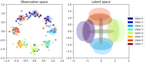
as-sume a zero-centred normal prior with unit variance and z ∈ R2. We optimise L(ind) with two inference models
qφ1(z|x1),qφ2(z|x2), and two separate likelihood func-tionspθ1(x1|z), pθ2(x2|z). Fig. 2a (right) shows the be-liefs of both information sources for 8 test data points. These test points are the means of the 8 mixture components of the observable data, rotated by2◦. The small rotation is only for visualisation purposes, since each source is allowed to per-ceive only one axis and would therefore produce indistin-guishable beliefs for data points with identical values on the perceived axis. We visualise the two beliefs corresponding to the same data point with identical colours. The height and width of the ellipses correspond to the standard deviations of the beliefs. Fig. 2a (left) shows random samples in the ob-servation space, generated from 10 random latent samples z∼qφm(z|xm)for each belief. The generated samples are colour-coded in correspondence to the figure on the right. The 8 circles in the background visualise the true data dis-tribution with 1 and 2 standard deviations. The two types of markers distinguish the information sourcesx1andx2used
for inference. As can be seen, the beliefs reflect the ambigu-ity as a result of perceiving a single dimensionxm.1
Next we integrate the two beliefs using Eq. (3). The re-sulting integrated belief and generated data from random latent samples of the belief are shown in Figs. 2b (right) and 2b (left) respectively. We can see that the integration resolves the ambiguity. In the supplementary material of our accompanying technical report (Kurle, G¨unnemann, and Smagt 2018), we plot samples from the individual and in-tegrated beliefs, before and after a sampling importance re-sampling procedure.
5.2
Learning and inference of shared
representations for structured prediction
Models trained withL(ind)orL(hybrid) can be used to
pre-dict structured data of any modality, conditioned on any available information source. Equivalently, we may impute missing data if modelled explicitly as an information source:
p(xm|xm0) =E
z∼qφm0 z|xm0
h
pθm(xm|z) i
. (6)
MNIST variants We created 3 variants of MNIST (Lecun et al. 1998), where we simulate multiple information sources as follows:
• MNIST-TB: x1 perceives thetophalf and x2 perceives
thebottomhalf of the image.
• MNIST-QU: 4 information sources that each perceive quartersof the image.
• MNIST-NO: 4 information sources with independent bit-flipnoisewithp= 0.05. We use these 4 sources to amor-tise inference. In the generative model, we use the stan-dard, noise-free digits as observable variables.
1
The true posterior (of a single source) has two modes for most data points. The uni-modal (Gaussian) proposal distribution learns to cover both modes.
(a) Individual beliefs and their predictions.Left:8 coloured cir-cles are centred at the 8 test inputs from a mixture of Gaussians toy dataset. The radii indicate 1 and 2 standard deviations of the normal distributions. The two types of markers represent gener-ated data from random samples of one of the information sources (data axis 0 or 1).Right:Corresponding individual beliefs. Ellipses show 1 standard deviation of the individual approximate posterior distributions.
(b) Integrated belief and its predictions.
Figure 2: Approximate posterior distributions and samples from the predicted likelihood function with and without in-tegration of beliefs
First, we assess how well individual beliefs can be inte-grated after learning, and whether beliefs can be used in-dividually when learning them as integrated inference distri-butions. On all MNIST variants, we train 5 different mod-els by optimising the objectivesL(ind),L(MoE),L(PoE), and
L(hybrid)withK= 16, as well asL(hybrid)withK= 1. All
other hyperparameters are identical. We then evaluate each model under the 3 objectives L(ind), L(MoE) andL(PoE).
For comparison, we also train a standard IWAE with hard-wired sources on MNIST and on MNIST-NO with a single noisy source. The ELBOs on the test set are estimated using
K = 16 importance samples. The obtained estimates are summarised in Tab. 1. The results confirm that learning the PoE inference model directly leads to inseparable individual beliefs. As expected, learning individual inference models and integrating them subsequently as a PoE comes with a tradeoff forL(PoE), which is mostly due to the low entropy
of the integrated distribution. On the other hand, optimising the model withL(hybrid) achieves good results for both
in-dividual and integrated beliefs. On MNIST-NO, we can get an improvement of 2.74nats by integrating the beliefs of redundant sources, compared to the standard IWAE with a single source.
Table 1: Negative evidence lower bounds on variants of ran-domly binarised MNIST. Lower is better.
MNIST-TB
L(ind) L(MoE) L(PoE) L(hybrid) L(hybrid) (K=1) IWAE
L(ind) 102.20 102.40 265.59 104.03 108.97 -L(MoE) 101.51 101.82 264.48 103.37 108.30 -L(PoE) 94.38 94.39 87.59 90.07 90.81 88.79
MNIST-QU
L(ind) L(MoE) L(PoE) L(hybrid) L(hybrid) (K=1) IWAE
L(ind) 120.46 120.37 447.67 129.63 140.61 -L(MoE) 119.10 119.98 446.02 128.16 139.19 -L(PoE) 108.07 107.85 87.67 89.20 90.17 88.79
MNIST-NO
L(ind) L(MoE) L(PoE) L(hybrid) L(hybrid) (K=1) IWAE
L(ind) 94.81 94.86 101.20 96.27 95.31 -L(MoE) 93.98 94.03 100.36 95.58 94.55 -L(PoE) 94.52 94.65 92.27 92.21 94.49 94.95
prediction using Eq. (6). Fig. 3a shows the means of the like-lihood functions, with latent variables drawn from individ-ual and integrated beliefs. To demonstrate conditional image generation from labels, we add a third encoder that perceives class labels. Fig. 3b shows the means of the likelihood func-tions, inferred from labels.
We also compare our method to the missing data im-putation procedure described in (Rezende, Mohamed, and Wierstra 2014) for MNIST-TB und MNIST-QU. We run the Markov chain for all samples in the test set for 150 steps each and calculate the log likelihood of the imputed data at every step. The results—averaged over the dataset— are compared to our multimodal data generation method in Fig. 4. For large portions of missing data as in MNIST-TB, the Markov chain often fails to converge to the marginal dis-tribution. But even for MNIST-QU with only a quarter of the image missing, our method outperforms the Markov chain procedure by a large margin. Please consult the supplemen-tary material for a visualisation of the stepwise generations during the inference procedure.
Caltech-UCSD Birds 200 Caltech-UCSD Birds 200
(Welinder et al. 2010) is a dataset with 6033 images of birds with128×128resolutions, split into 3000 train and 3033 test images. As a second source, we use segmentation masks provided by (Yang, Safar, and Yang 2014). On this dataset we assess whether learning with multiple modalities can be advantageous in scenarios where we are interested only in one particular modality. Therefore, we evaluate the ELBO for a single source and a single target observation, i.e. encod-ing images and decodencod-ing segmentation masks. We compare models that learned with multiple modalities using L(ind)
andL(hybrid)with models that learnt from a single modality.
Additionally, we evaluate the segmentation accuracy using Eq. (6). The accuracy is estimated with 100 samples, drawn from the belief informed by image data. The results are sum-marised in Tab. 2. We distinguish between objectives that in-volve both modalities in the generative model and objectives where we learn only the generative model for the modality
(a) Row 1: Original images.
Row 2–4:Belief informed by top half of the image.Row 5–7:
Informed by bottom half.Row 8–10:Integrated belief.
(b) Predictions from 10 random samples of the latent variables, inferred from one-hot class la-bels.
Figure 3: Predicted images, where latent variables are in-ferred from the variational distributions of different sources. Sources with partial information generate diverse samples, the integration resolves ambiguities. E.g. in Fig. 3a, the lower half of digit 3 randomly generates digits 5 and 3 and the upper half generates digits 3 and 9. In contrast, the inte-gration resolves ambiguities.
(a) MNIST-TB, where bottom half is missing.
(b) MNIST-QU, where bottom right quarter is missing.
Figure 4: Missing data imputation with Monte Carlo proce-dure described in (Rezende, Mohamed, and Wierstra 2014) and our method. For the Markov chain procedure, the ini-tial missing data is drawn randomly fromBer (0.5)and im-puted from the previous random generation in subsequent steps. MSNVI was trained withL(ind). For MNIST-QU, we
used the PoE belief of the three observed quarters. The plots show the log-likelihood at every step of the Markov chain, marginalised over the dataset. Higher is better.
Table 2: Negative ELBOs and segmentation accuracy on Caltech-UCSD Birds 200. The IWAE was trained with a single source and target observation. Models trained with
L(ind)andL(hybrid)use all sources and targets, andL(ind)*
and L(hybrid)* use all sources for inference, but learn the
generative model of a single modality.
L(ind) L(ind)* L(hybrid) L(hybrid)* IWAE
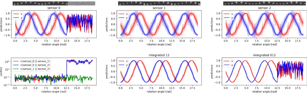
Figure 5: Predictions (x- andy-coordinates) of the pendulum position (figures 1, 2, 3, 5, 6) and conflict measure (figure 4). For the predictions, latent variables are inferred from images of 3 sensors with different views (top row) as well as their integrated beliefs (bottom mid and right). The figures show predictions (of the static model) for different angles of the pendulum, performing 3 rotations. After 2 rotations, failure of sensor 0 is simulated by outputting noise only. Lines show the mean and shaded areas show 1 and 2 standard deviations, estimated using 500 random samples of latent variables. Bottom left: The conflict measure of Eq. (2) for different angles of the pendulum.
of interest (segmentation), denoted with an asterisk. Mod-els that have to learn the generative modMod-els for images and segmentations show worse ELBOs and accuracy, when eval-uated on one modality. In contrast, the accuracy is slightly increased when we learn the generative model of segmenta-tions only, but use both sources for inference.
We also refer the reader to the supplementary material of our technical report (Kurle, G¨unnemann, and Smagt 2018), where we visualise conditionally generated images, show-ing that learnshow-ing with the importance samplshow-ing estimate of the ELBO is crucial to generate diverse samples from par-tially informed sources.
5.3
Robustness via conflict detection and
redundancy
In this experiment we demonstrate how a shared latent rep-resentation can increase robustness, by exploiting sensor re-dundancy and the ability to detect conflicting data. We cre-ated a synthetic dataset of perspective images of a pendulum with different views of the same scene. The pendulum ro-tates along the z-axis and is centred at the origin. We simu-late three cameras with32×32-pixel resolution as informa-tion sources for inference and apply independent noise with std0.1to all sources. Each sensor is directed towards the ori-gin (centre of rotation) from different view-points: Sensor 0 is aligned with thez-axis, and sensor 1 and 2 are rotated by
45 deg along thex- andy-axis, respectively. The distance of all sensors to the origin is twice the radius of the pen-dulum rotation. For the generative model we use thex- and
y-coordinate of the pendulum rather than reconstructing the images. The model was trained withL(ind).
In Fig. 5, we plot the mean and standard deviation of pre-dictedx- and y-coordinates, where latent variables are in-ferred from a single source as well as from the PoE posteri-ors of different subsets. As expected, integrating the beliefs
from redundant sensors reduces the predictive uncertainty. Additionally, we visualise the three images used as informa-tion sources above these plots.
Next, we simulate an anomaly in the form of a defect sen-sor 0, outputting random noise after 2 rotations of the pen-dulum. This has a detrimental effect on the integrated be-liefs, where sensor 0 is part of the integration. We also plot the conflict measure of Eq. (2). As can be seen, the conflict measures for sensor 0 increases significantly when sensor 0 fails. In this case, one should integrate only the two remain-ing sensors with low conflict conjunctively.
6
Summary and future research directions
We extended neural variational inference to scenarios where multiple information sources are available. We proposed an objective function to learn individual inference models jointly with a shared generative model. We defined an ex-emplar measure (of conflict) to compare the beliefs from distinct inference models and their respective information sources. Furthermore, we proposed a disjunctive and a con-junctive integration method to combine arbitrary subsets of beliefs.
We compared the proposed objective functions exper-imentally, highlighting the advantages and drawbacks of each. Naive integration as a PoE (L(PoE)) leads to
insepa-rable individual beliefs, while optimising the sources only individually (L(ind)) worsens the integration of the sources.
On the other hand, a hybrid of the two objectives (L(hybrid))
achieves a good trade-off between both desiderata. More-over, we showed how our method can be applied to struc-tured output prediction and the benefits of exploiting the comparability of beliefs to increase robustness.
about the type of information source. Interesting research directions are extensions to sequence models, hierarchical models and different forms of information sources such as external memory. Another important research direction is the combination of disjunctive and conjunctive integration methods, taking into account the conflict between sources.
Acknowledgements
We would like to thank Botond Cseke for valuable sugges-tions and discussions.
References
Andrew, G.; Arora, R.; Bilmes, J.; and Livescu, K. 2013. Deep canonical correlation analysis. InProceedings of the 30th Interna-tional Conference on InternaInterna-tional Conference on Machine Learn-ing - Volume 28, ICML’13, III–1247–III–1255. JMLR.org. Bach, F., and Jordan, M. 2005. A probabilistic interpretation of canonical correlation analysis.
Baltruˇsaitis, T.; Ahuja, C.; and Morency, L.-P. 2017. Multi-modal machine learning: A survey and taxonomy. arXiv preprint arXiv:1705.09406.
Bousquet, N. 2008. Diagnostics of prior-data agreement in applied Bayesian analysis.Journal of Applied Statistics35(9):1011–1029. Burda, Y.; Grosse, R. B.; and Salakhutdinov, R. 2015. Importance weighted autoencoders.CoRRabs/1509.00519.
Cremer, C.; Li, X.; and Duvenaud, D. K. 2018. Inference subopti-mality in variational autoencoders.CoRRabs/1801.03558. Dahl, F. A.; G˚asemyr, J.; and Navig, B. A robust conflict measure of inconsistencies in Bayesian hierarchical models. Scandinavian Journal of Statistics34(4):816–828.
Dempster, A. P. 1967. Upper and lower probabilities induced by a multivalued mapping.Ann. Math. Statist.38(2):325–339. Deng, Y. 2015. Generalized evidence theory.Applied Intelligence
43(3):530–543.
Denœux, T. 2008. Conjunctive and disjunctive combination of be-lief functions induced by nondistinct bodies of evidence.Artificial Intelligence172(2):234 – 264.
Feng, F.; Li, R.; and Wang, X. 2015. Deep correspondence re-stricted boltzmann machine for cross-modal retrieval. Neurocom-puting154:50–60.
Gershman, S., and Goodman, N. D. 2014. Amortized inference in probabilistic reasoning. InProceedings of the 36th Annual Meet-ing of the Cognitive Science Society, CogSci 2014, Quebec City, Canada, July 23-26, 2014.
Hardoon, D. R.; Szedmak, S. R.; and Shawe-taylor, J. R. 2004. Canonical correlation analysis: An overview with application to learning methods.Neural Comput.16(12):2639–2664.
Hinton, G. E. 2002. Training products of experts by minimizing contrastive divergence.Neural Comput.14(8):1771–1800. Hotelling, H. 1936. Relations between two sets of variates.
Biometrika28(3/4):321–377.
Jiang, W.; Xie, C.; Zhuang, M.; Shou, Y.; and Tang, Y. 2016. Sen-sor data fusion with z-numbers and its application in fault diagno-sis.Sensors16(9).
Khaleghi, B.; Khamis, A.; Karray, F.; and Razavi, S. 2013. Multi-sensor data fusion: A review of the state-of-the-art. 14.
Kingma, D. P., and Welling, M. 2013. Auto-encoding variational Bayes.CoRRabs/1312.6114.
Kurle, R.; G¨unnemann, S.; and Smagt, P. v. d. 2018. Multi-Source Neural Variational Inference. ArXiv e-printsabs/1811.04451. Lecun, Y.; Bottou, L.; Bengio, Y.; and Haffner, P. 1998. Gradient-based learning applied to document recognition. Proceedings of the IEEE86(11):2278–2324.
Mnih, A., and Gregor, K. 2014. Neural variational inference and learning in belief networks. In Proceedings of the 31th Inter-national Conference on Machine Learning, ICML 2014, Beijing, China, 21-26 June 2014, 1791–1799.
Murphy, C. K. 2000. Combining belief functions when evidence conflicts.Decis. Support Syst.29(1):1–9.
Ngiam, J.; Khosla, A.; Kim, M.; Nam, J.; Lee, H.; and Ng, A. Y. 2011. Multimodal deep learning. In Getoor, L., and Scheffer, T., eds.,ICML, 689–696. Omnipress.
Rasiwasia, N.; Costa Pereira, J.; Coviello, E.; Doyle, G.; Lanckriet, G. R.; Levy, R.; and Vasconcelos, N. 2010. A new approach to cross-modal multimedia retrieval. InProceedings of the 18th ACM International Conference on Multimedia, MM ’10, 251–260. New York, NY, USA: ACM.
Rezende, D. J.; Mohamed, S.; and Wierstra, D. 2014. Stochas-tic backpropagation and approximate inference in deep generative models. InProceedings of the 31th International Conference on Machine Learning (ICML), 1278–1286.
Shafer, G. 1976. A Mathematical Theory of Evidence. Princeton: Princeton University Press.
Shon, A. P.; Grochow, K.; Hertzmann, A.; and Rao, R. P. N. 2005. Learning shared latent structure for image synthesis and robotic imitation. In Proceedings of the 18th International Conference on Neural Information Processing Systems, NIPS’05, 1233–1240. Cambridge, MA, USA: MIT Press.
Srivastava, N., and Salakhutdinov, R. 2014. Multimodal learning with deep boltzmann machines. Journal of Machine Learning Re-search15:2949–2980.
Stein, B. E., and Meredith, M. A. 1993.The merging of the senses. Cambridge, MA, US: The MIT Press.
Suzuki, M.; Nakayama, K.; and Matsuo, Y. 2016. Joint multimodal learning with deep generative models.
Vedantam, R.; Fischer, I.; Huang, J.; and Murphy, K. 2017. Generative models of visually grounded imagination. CoRR
abs/1705.10762.
Welinder, P.; Branson, S.; Mita, T.; Wah, C.; Schroff, F.; Belongie, S.; and Perona, P. 2010. Caltech-UCSD Birds 200. Technical Report CNS-TR-2010-001, California Institute of Technology. Wu, M., and Goodman, N. 2018. Multimodal generative models for scalable weakly-supervised learning.CoRRabs/1802.05335. Yang, J.; Safar, S.; and Yang, M.-H. 2014. Max-margin boltz-mann machines for object segmentation. 2014 IEEE Conference on Computer Vision and Pattern Recognition320–327.
Zadeh, L. A. 1986. A simple view of the dempster-shafer theory of evidence and its implication for the rule of combination. AI Mag.