Efficient Identification of Approximate Best Configuration of Training in Large Datasets

The Thirty-Third AAAI Conference on Artificial Intelligence (AAAI-19)

Efficient Identification of Approximate

Best Configuration of Training in Large Datasets

Silu Huang,

_{Chi Wang,}

_{Bolin Ding,}

_{Surajit Chaudhuri}

2_{Microsoft Research, Redmond, WA} 3_{Alibaba Group, Bellevue, WA}

[email protected],{wang.chi, surajitc}@microsoft.com, [email protected]

Abstract

A configuration of training refers to the combinations of fea-ture engineering, learner, and its associated hyperparameters. Given a set of configurations and a large dataset randomly split into training and testing set, we study how to efficiently identify the best configuration with approximately the high-est thigh-esting accuracy when trained from the training set. To guarantee small accuracy loss, we develop a solution using confidence interval (CI)-based progressive sampling and prun-ing strategy. Compared to usprun-ing full data to find the exact best configuration, our solution achieves more than two orders of magnitude speedup, while the returned top configuration has identical or close test accuracy.

Introduction

Increasing the productivity of data scientists has been a target for many machine learning service providers, such as Azure ML, DataRobot, Google Cloud ML, and AWS ML. For a new predictive task, a data scientist usually spends a vast amount of time to train a good ML solution. A properconfiguration, i.e., the combination of preprocessing, feature engineering, learner (i.e., training algorithm) and the associated hyper-parameters, is critical to achieving good performance. It usually takes tens or hundreds of trials to select a suitable configuration.

There are AutoML tools like auto-sklearn (Feurer et al. 2015) to automate these trials, and output a configuration with highest evaluated performance. However, both the man-ual and AutoML approaches have become increasingly inef-ficient as the available ML data volume grows to millions or more. Even the trial for a single configuration can take hours or days for such large-scale datasets. Motivated by this effi-ciency issue, we propose a module calledapproximate best configuration(ABC). Given a set of configurations, it outputs the approximate best configuration, such that the accuracy loss to the best configuration is below a threshold. Our goal is toefficientlyidentify the approximate best configuration.

The intuition behind ABCis that the ML model trained

over a sampled dataset can be used to approximate the model trained over the full dataset. However, the optimal sample

∗

Work done while visiting Microsoft Research †

Work done while working in Microsoft Research

Copyright c2019, Association for the Advancement of Artificial Intelligence (www.aaai.org). All rights reserved.

size to determine the best configuration up to an accuracy loss threshold is unknown. We develop a novel confidence interval (CI)-based progressive sampling and pruning solu-tion, by addressing two questions:(a) CI estimator:given a sampled training dataset, how to estimate the confidence in-terval of a configuration’s real performance with full training data?(b) scheduler:as the optimal sample size is unknown

a priori, how to allocate appropriate sample size for each configuration?

Our contributions are summarized as the following.

• We develop an ABC framework using progressive sam-pling and CI-based pruning. It ensures finding an approxi-mate best configuration while reducing the running time.

• We present and prove bounds for the real test accuracy when the ML model is trained using full data, based on the model trained with sampled data.

• Within ABC, we design an approximately optimal schedul-ing scheme based on the confidence interval, for allocatschedul-ing sample size among different configurations.

• We conduct experiments with large datasets. We demon-strate that our ABCsolution is tens to hundreds of times faster, while returning top configurations with no more than 1% accuracy loss.

Problem Formulation

Notions and Notations. In this paper, we focus on classi-fication tasks with a large set of labeled dataD. In order for reliable evaluation of a trained classifier, data scientists usually split the available datarandomlyinto training and testing setDtr andDte. After that, they specify a number

of configurations of the ML workflow and try to identify the best configuration. LetCbe the candidate configuration set andCi be theith configuration inC. We further let nbe

the number of configurations, i.e.,n=|C|. Using terminol-ogy from learning theory, each configurationCi defines a

hypothesis spaceHi, where eachhypothesisH ∈ Hiis a

possible classifier trained under this configuration. Given a training datasetDtr, the learner inCiwill output a

hypoth-esisHi

tr ∈ Hi as the trained classifier. The quality of the

classifier is measured against the heldout testing dataDte. In

|D| |F | Origin

Twitter 1.4M 9866 Twitter, Stanford FlightDelay 7.3M 630 U.S. Department of

Transportation NYCTaxi 10M 21 NYC Taxi &

Limou-sine Commission

HEPMASS 10M 28 UCI

HIGGS 10.6M 28 UCI

Table 1: Dataset Description

A(H, D). In particular, given a configurationCi, we define

itsreal test accuracyasAi=A(Htri ,Dte).

Problem Definition. A standard practice to select the best configuration from a configuration setCis to train with each configuration using full training data, and then pick the one with the highest test accuracy, i.e.,Ci∗= arg max_C

i∈C{Ai}.

Note that an implicit assumption made here is that the re-turned classifier with full training data has equal or higher test accuracy than the classifier trained with sampled training data. We call thisexploitativenessassumption and follow it in this paper. From a user’s perspective, if there are multiple configurations with nearly identical highest real test accuracy, then it would suffice to return any of them as the best config-uration. So we introduce a new problemapproximate best configurationidentification, as formalized in Problem 1.

Problem 1(Approximate Best Configuration Identification).

Given a configuration candidate setCand an accuracy loss tolerance, identify a configurationCi0 whose real test

accu-racy is withinaway from that of the best configurationCi∗,

i.e.,Ai∗− A_i0 ≤, and minimize the total running time.

CI-based Framework

Before introducing our framework, we first describe some insights based on simple observations. We experiment on the

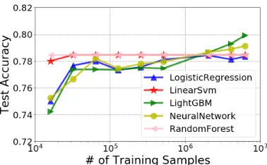
FlightDelaydataset published in Azure Machine Learning gallery (Mund 2015) with five learners (as five configura-tions). Readers can refer to Table 1 for detailed statistics of this dataset, where|D|and|F |is the number of records and features respectively. Thelearning curvefor each configu-ration is depicted in Figure 1, where x-axis is the training sample size in log-scale and y-axis is the test accuracy on Dte. In general, the test accuracy approaches the real test

accuracy with the increase of the training sample size. When the sample size is large enough (>2M), the configuration with the highest test accuracy is LightGBM – the true best configuration.

Furthermore, the optimal sample size to minimize the run-ning time could vary for different configurations. If we mag-ically know that we should use 2M training samples for LightGBM and 16K training samples for all the other config-urations, we can save even more time and still identify the correct best configuration. Unfortunately, the optimal sample size for each configuration is unknown. A natural idea is to increase the sample size gradually, until a plateau is reached in the learning curve. However, a naive plateau estimator based on the learning curve is error-prone. As shown from

Figure 1: Learning Curve

Figure 1, LightGBM’s learning curve is flat from 32K to 128K. If we stop increasing the sample size for it, it will be mis-pruned. Therefore, a more robust strategy is needed. Overview. The main idea is to estimate theconfidence in-terval(CI) of each configuration’s real test accuracy with sampled data, instead of simply using a point estimation of the real test accuracy. In each round, we train the classifier for a selected configuration on some sampled training data. We call such a round of training aprobe. After a probe, we update the confidence interval for the configuration. As the sample size increases, the confidence interval shrinks, and the badly-performing configurations can be pruned based on the CIs. The pruning based on CI is more robust than based on random observations from the learning curve.

Algorithm 1:ABC

1 Input:configuration setC, accuracy loss threshold; 2 Output:the approximate best configuration;

3 Initialization:Cprob←C1,Ci0 ←C1,Ω← C;

4 while|Ω|>1do

5 PROBE(Cprob);

6 [Cprob.l, Cprob.u]←CIESTIMATOR(Cprob) ;

7 ifCprob.l > Ci0.lthen C_i0 ←C_prob;

8 forC∈Ωdo // pruning

9 ifC.u−Ci0.l≤then Ω←Ω−C;

10 ifPruning happensthen

11 forC∈Ωdo

12 C.u_old←C.u;C.lold←C.l;

13 C_prob←SCHEDULER(Ω)

14 returnCi0;

Detailed Algorithm. ABC proceeds round by round as shown in Algorithm 1, where each configurationCiis

anno-tated with its current sample size (Ci.s), current lower bound

(Ci.l), current upper bound (Ci.u), and the snapshot of lower

bound (Ci.lold) and upper bound (Ci.uold) in the last

prun-ing round. In each round within the while loop (line 4), it first probes the configurationCprob(line 5). Then it calls a

CIESTIMATORsubroutine to quickly estimate the confidence interval forAprob(line 6). Next, it prunes badly-performing

configurations (line 7-9). Line 7 identifies the configuration

Ci0 with the largest lower bound. Line 8-9 prunes an

lower bound. If there exists configuration being pruned (line 10), we call this iteration asnapshotand will updateC.lold

andC.uoldfor each configurationCin this snapshot (line

11-12). At last, it calls a SCHEDULERsubroutine to determine which configuration to probe next as well as its sample size (line 10).

We describe CIESTIMATORand SCHEDULERin the next two sections.

CI Estimator

In this section, we will derive a CIESTIMATOR for each configuration’s real test accuracy, based on the probe over sampled data. For configurationCi, the confidence interval

[li, ui]needs to contain the real test accuracyAiwith high

probability. The computation oflianduineeds to be efficient,

i.e., no slower than the probe. In the following, we assumei

is fixed and omit it in the notations.

At the first glance, the CI estimation may remind readers of the generalization error bounds (e.g., VC-bound). The generalization error bound is a universal bound of the differ-ence between each hypothesis’s accuracy in training data and its accuracy in infinite data following the same distribution. Nevertheless, the confidence interval we need is the range of the real test accuracy of the hypothesisHtrtrained from

full training data, while we only have the hypothesisHStr

trained from a sampleStr ⊂ Dtr. Therefore, we cannot

apply generalization error bound to obtain our confidence interval.

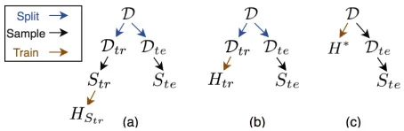
We use Figure 2 to summarize the notations and their relationships which are important for understanding the theo-retical results.Htr,HStr, andH

∗_{correspond to the returned}

hypothesis after training a fixed configuration with full train-ing datasetDtr, the sampled training dataset Str, and the

full dataDrespectively. For instance, Figure 2(a) shows the overall derivation relationships amongD,Dtr,Dte,Str,Ste,

andHStr. First, the full training dataDtrand the full testing

dataDteare randomly split from the whole dataD. Second,

the sampled training dataStrand the sampled testing data

Steare randomly drawn from the full training dataDtrand

full testing dataDte. Last,HStr is trained from the sampled

training dataStr. Note that the CI estimator only has access

toHStr, StrandSte. ThoughHtrandH

∗_{are not accessible,}

they are useful in our analysis.

Upper bound.The intuition behind the confidence interval estimation is that we need to relate the two hypothesesHStr

andHtr, and use the information we have onHStrto infer the

performance ofHtr. To upper bound the accuracy ofHtr, we

leverage afitnesscondition: the training process produces a hypothesis that fits the training data. When the configuration is fixed, the accuracy in a datasetDof the hypothesis trained onDshould be no worse than the hypothesis trained on a different datasetD0_{6=D. It is the only assumption we need}

to prove the upper bound, no matter what training algorithm is used. Under this condition, we found an inequality chain to connect the training accuracyA(HStr, Str)to the real test

accuracy ofHtr.

Theorem 1(Upper Bound). Under the fitness condition, with

Figure 2: Notations Used in CI Estimation and Analysis

probability at least1− δ

2n2,A(Htr,Dte)≤u, where

u_,A(HStr, Str) + ( 1 2|Str|

ln4n

2

δ ) 1

2 + ( 1

2|Dte|

ln4n

2

δ ) 1 2

Proof. Let us first recall the fitness condition. Given a fixed configurationCi, letHandH0be the hypothesis returned by

training on two different sample setsDandD0, respectively. Note thatH andH0are both from the same fixed hypothesis spaceHi. Our assumption is thatHhas no lower accuracy

onDthanH0. Similarly,H0has no lower accuracy onD0

thanH.

First, let us break downA(Htr,Dte)− A(HStr, Str)into

four clauses, as shown in Equation (1).

A(Htr,Dte)− A(HStr, Str)

=[A(Htr,Dte)− A(H∗,Dte)] + [A(H∗,Dte)− A(H∗,D)]+ A(H∗,D)− A(H∗, Str)] + [A(H∗, Str)− A(HStr, Str)]

(1)

SinceDtr andDte are randomly split fromD, we have

D=Dtr∪ Dte. Letx= |D_|D|te|be the hold-out ratio. For any

H ∈ H, we have:

xA(H,Dte) + (1−x)A(H,Dtr) =A(H,D)

⇒ A(H,Dte) =

1

x[A(H,D)−(1−x)A(H,Dtr)]

(2)

Next, apply Equation (2) to the first clause in Equation (1):

A(Htr,Dte)− A(H∗,Dte)

=1

x[A(Htr,D)− A(H

∗_,D)]−1−x

x [A(Htr,Dtr)

− A(H∗,Dtr)]≤0

(3)

The inequality is derived from the fitness assumption (recall from Figure 2Htris trained fromDtrandH∗is trained from

D).

Next, we bound the second clause in Equation (1) with Hoeffding inequality: With probability at least(1− δ

4n2),

A(H∗,Dte)− A(H∗,D)≤(

1 2|Dte|

ln4n

2

δ ) 1 2 (4)

Similarly, with probability at least(1− δ

4n2),

A(H∗,D)− A(H∗, Str)≤(

1 2|Str|

ln4n

2

δ ) 1 2 (5)

DteandStr cannot be regarded as random samples, since

HStris tailored to the sample setStr. Therefore, introducing

H∗_{is necessary in our analysis.}

Last, sinceHStris trained fromStr, by the fitness

assump-tion we have:

A(H∗, Str)− A(HStr, Str)≤0 (6)

By substituting the four clauses in Equation (1) with Equa-tion (3)-(6), we obtain Theorem 1 using union bound.

Note that the computation ofA(HStr, Str)is no slower

than the probing (i.e., training with sampled data). In fact, the evaluation is usually much more efficient than training for the same scale of dataset.

Lower Bound.The lower bound is easier due to the exploita-tivenesspresumption discussed in the problem formulation: Full training data produce better hypothesis than sampled training data for a fixed configuration. The real test accuracy ofHtrcan then be lower bounded byA(HStr, Dte).

How-ever, the computation ofA(HStr, Dte)can be slower than

probing, if|Dte| |Str|. To make the CI estimation

effi-cient, we also sample the testing data. We denote the sampled testing data asSte. We can then lower boundA(HStr, Dte)

byA(HStr, Ste)minus a variation term.

Theorem 2(Lower Bound). Under the exploitativeness as-sumption, with probability at least1− δ

2n2,

A(Htr,Dte)≥l,A(HStr, Ste)−( 1 2|Ste|

ln2n

2

δ ) 1 2

Proof. First, in the problem formulation we have assumed

A(Htr,Dte)≥ A(HStr,Dte) (7)

Next, based on Hoeffding inequality, with probability at least

1− δ

2n2,

A(HStr, Ste)− A(HStr,Dte)≤( 1 2|Ste|

ln2n

2

δ ) 1 2 (8)

Combining Equation (7) and (8), we haveA(Htr,Dte)≥l

with probability at least1− δ

2n2.

CIESTIMATORin Algorithm 1.With Theorem 1 and 2, we can now estimate the current lower bound and upper bound of the probing configurationCprob. As shown in Algorithm 2,

we first initialize the current lower boundCprob.land

up-per boundCprob.uaccording to Theorem 1 and 2.

Further-more, we add a constraint that the current CI must be con-tained in the CI of the last snapshot where pruning happens, i.e., [Cprob.l, Cprob.u] ⊂ [Cprob.lold, Cprob.uold]. Thus, if

Cprob.l < Cprob.lold, we replace Cprob.l with Cprob.lold

(line 4). Similar forCprob.u(line 5). In this way, we can

guarantee that the CI for each configuration shrinks from one snapshot to another snapshot where pruning happens. Recall thatCprob.loldandCprob.uoldget updated in each snapshot.

Algorithm 2:CIESTIMATOR

1 Input:C_prob,A_prob(H_Str, S_tr),A_prob(H_Str, S_te);

2 Output:[Cprob.l, Cprob.u];

3 [C_prob.l, C_prob.u]←Theorem 1 and 2 ;

4 ifCprob.l < Cprob.loldthenCprob.l←Cprob.lold;

5 ifCprob.u > Cprob.uoldthenCprob.u←Cprob.uold;

6 return[Cprob.l, Cprob.u];

Correctness of Algorithm 1

Using Algorithm 2, we can estimate the confidence interval for the real test accuracy, based on each probe over the sam-pled training dataStrand the sampled testing dataSte. Next,

Theorem 3 shows that Algorithm 1 can successfully return an approximate best configuration with high probability.

Corollary 1(Confidence Interval). With probability at least

1− δ

n2, Ai∈[li, ui].

Theorem 3(Correctness). With probability at least1−δ, Algorithm 1 returns the approximate best configurationCi0

withAi∗− A_i0 ≤.

Proof. Without loss of generality, we assumeC1is the re-turned configurationCi0by Algorithm 1. We denote the

iter-ations in Algorithm 1 with at least one configuration pruned, i.e., snapshots, as setR. We will prove that when all the con-fidence intervals at iterationsRcorrectly bound the real test accuracy (denoted as eventE), the algorithm returns correct approximate configuration. We show that whenEhappens, for each pruned configuration2≤i≤n,Ai≤ A1+.

Consider iterationr ∈ Rand letl(_ir)

r be the the highest

lower bound in this iteration, andCpr be a pruned

config-uration in iterationr. WhenEhappens,Apr ≤upr. And

upr ≤ l

(r)

ir +according to line 9 in Algorithm 1. So the

pruned configuration must satisfyApr ≤l

(r)

ir +.

Further-more, as Algorithm 1 proceeds to iterationr+1,l(_ir)

r ≤l

(r+1)

ir+1 .

This is because the lower bound of configurationCir does

not decrease from snapshotrto snapshotr+ 1according to Algorithm 2, i.e.,l(_ir)

r ≤l

(r+1)

ir .In addition,l

(r+1)

ir ≤l

(r+1)

ir+1

in snapshotr+ 1, according to line 7 in Algorithm 1. Thus, Apr ≤l1+by induction on the iteration numberr. Also,

sincel1+≤ A1+, we haveApr ≤ A1+.

Next, letErbe the event that all the confidence intervals

at iterationrcorrectly bound the real test accuracy where

r∈R. We can decompose eventE¯into non-overlapping sub-events{E¯1,E¯2|E1,E¯3|E2,· · · }, whereE¯(resp. E¯r) is the

opposite event ofE(resp.Er). According to Corollary 1, the

derived confidence interval[li, ui]is correct with probability

at least1− δ

n2 for any configurationCi. Hence, the

proba-bility ofE¯r+1|Eris at most _nδ according to Algorithm 2 and

the union bound. Furthermore, we haven−1pruned config-urations across all iterations, so|R|< n. Consequently, the probability ofE¯ is at mostδby summing up the probability of non-overlapping sub-eventsE¯r+1|Er. That is, eventE

Discussion.We have used the exploitativeness assumption in deriving the lower bound: Ai(HStr, Dte)≤ Ai(Htr, Dte)

for anyCi. We argue that even though this assumption is

not exactly satisfied in practice, it holds closely enough to provide useful results. That is, in most cases this assumption holds, and even when this assumption is violated, we can perform a post-processing step after the algorithm finishes. If there existsAi0(H_S

tr, Dte)> Ai0(Htr, Dte)for the

se-lected configurationCi0, the user could useH_S

tr instead of

Htr as the final classifier. First, that satisfies users’

prefer-ence in finding a more accurate classifier. Second, it holds the-guarantee, because the lower boundli0holds forH_S

tr

of configurationCi0, and it is no lower than the pruning lower

boundslir,∀r∈R.

The correctness of our algorithm is independent of the choice of the scheduler.

Scheduler

Now we have shown that our proposed ABC can identify the approximate best configuration with high probability. This section focuses on the optimization part in Problem 1, i.e., how to minimize the total running time. LetTi(s)be

the probing time with a sampled training dataset sizesfor configurationCi, andti be the accumulated running time

for probing configurationCi in Algorithm 1. Also, letli

andui be the lower bound and upper bound respectively

for configurationCi when the algorithm terminates. With

these notations, the design of SCHEDULERin ABCcan be expressed as a constrained optimization problem. Without loss of generality, assumeC1is returned by Algorithm 1. Problem 2(Scheduling). Design a scheduler to minimize

T =P

iti, subject to:

u2≤l1+, u3≤l1+, . . . , un≤l1+

The objective function in Problem 2 is the time taken to identify the approximate best configuration. Since probing dominates the running time in each iteration, we use the total time of all probes as the proxy of the identification time. The constraints in Problem 2 ensure that all the configurationsCi

are pruned exceptC1, and are necessary for the termination of Algorithm 1.

To solve Problem 2, we begin with studying the properties of the ‘oracle’ optimal scheduling scheme when it has access toti as a function oflianduirespectively, i.e.,ti =fi(li)

andti = gi(ui), after the samples are drawn. We claim

that the optimal scheduling scheme with this oracle access probes each configuration uniquely once, since otherwise we can always reduce the total running time by only keeping the last probe. Our objective function can be rewritten as

f1(l1) +g2(u2) +· · ·+gn(un). Furthermore, by applying

the method of Lagrange multipliers, we obtain the conditions the optimal solution must satisfy:

  

df1

dl1 =−(

dg2

du2 +· · ·+

dgn

dun)

l1+=u2=· · ·=un

(9)

Now, since we do not have oracle access tofiandgi, there

is no closed-form formula to decide the optimal sample size

s∗_i for configurationCi. To solve this challenge, We propose

a scheduling scheme GRADIENTCI with two parts.

First, we use the gradient of the running time with respect to the confidence interval to determine the configuration to probe next. We depict this strategy in Algorithm 3. GRA

-DIENTCI first sorts the remaining configuration setΩ in descending order of the upper bound (line 3), and make a guess (Ω1) on the best configurationC1. Next, it compares the gradient∆T1

∆l1 with|

∆T2

∆u2 +· · ·+

∆Tn

∆un|: If

∆T1

∆l1 is smaller,

then configurationΩ1with the largest upper bound is picked for the next probe (line 4); otherwise, configurationΩ2with the second largest upper bound is picked (line 5). Here,∆Ti

denotes the running time difference between the recent two consecutive probes onCi, and ∆_∆T_lii serves as the proxy of

∆fi

∆li (similar for

∆gi

∆ui). The choice betweenΩ1and others is

based on the first condition in Equation (9). Intuitively, if the lower bound ofΩ1grows faster (per time spent) than all the other configurations’ upper bounds’ decrease, then we opt to probeΩ1. The choice ofΩ2amongΩ2toΩnis based on the

second condition in Equation (9), towards attaining the same upper bound for them.

Second, we design the sample size sequence within each configuration. As shown in line 6 of Algorithm 3, we utilize a common trick called geometric scheduling, which was used in prior work to increase the sample size for a single configuration (Provost, Jensen, and Oates 1999). We further derive the closed-form for the optimal step sizec, whenTi(s)

is a power function over the sample size, i.e.,Ti(s) = sα

whereαis a real number. The optimal step size follows

c= 2α1. Details can be found in our technical report (Huang

et al. 2018).

Algorithm 3:SCHEDULER–GRADIENTCI

1 Input:Remaining configurationsΩ;

2 Output:Configuration for next probeC_prob; 3 sort by upper bound(Ω);

4 if ∆T1

∆l1 ≤ |

∆T2

∆u2 +· · ·+

∆Tn

∆un|then Cprob←Ω1;

5 else Cprob←Ω2;

6 Cprob.s←c×Cprob.s;

7 returnCprob;

Performance Analysis.In practice, ABCis used in two sce-narios. Scenario (i): during exploration, users want to try a few configurations (e.g., verifying usefulness of a few new features) as an intermediate step. The identification result will decide the follow-up trials, but it does not serve as the final configuration, and does not require full training ofCi0.

Sce-nario (ii): at the end of the exploration, users need to get the trained classifier corresponding to the selected configuration

Ci0. In scenario (ii), the total running time involves not only

the time to identify the approximate best configuration, but also the time taken to train the classifier on full data withCi0.

WhenCi0is fixed, both scenario (i) and (ii) share the same

Experiments

This section evaluates the efficiency and effectiveness of our ABCmodule. First, we evaluate whether ABCsuccessfully identifies top configuration and meanwhile reduce the total running time. Second, we compare the CI-based pruning with an existing pruning algorithm based on point estimation. We also compare different scheduling schemes in our technical report (Huang et al. 2018).

Experimental Setup

Configurations. We focus on the task of classifying fea-turized data in our evaluation. Specifically, we choose five widely used and high-performance learners: LogisticRegres-sion, LinearSVM, LightGBM, NeuralNetwork,and Random-Forest. Each classifier is associated with various hyperpa-rameters, e.g., the number of trees in RandomForest and the penalty coefficient in LinearSVM. In total they have 29 dis-crete or continuous hyperparameters. In our experiments, we use random search to generate each hyperparameter value from its corresponding domain.

Datasets.We evaluate with five large-scale machine learn-ing benchmarks that are publicly available. As discussed in introduction, the motivation of ABC is to handle large datasets and quickly identify the approximate best configura-tion. Thus, the datasets evaluated in our experiments are all at the scale of millions of records (|D|) and with up to 10K fea-tures (|F |). We do not use the AutoML benchmarks such as HPOlib (Eggensperger et al. 2013) or OpenML (Vanschoren et al. 2013), which mainly contain small or median-sized datasets (up to 50K records). The statistics of each dataset are depicted in Table 1. We used min-max normalization for all datasets, and n-gram extraction as well as model-based top-K feature selection for Twitter.

Algorithms.We compare our proposed ABCwith the stan-dard approach namedFull-run. For each configuration, Full-run first trains the classifier with full training data, and then tests it on the full testing data. Afterwards, it returns the con-figuration with the highest testing accuracy. This method is supported in mature tools like scikit-learn and Azure ML. Existing approaches to best configuration identification, such as DAUB (Sabharwal, Samulowitz, and Tesauro 2016) or successive-halving (Jamieson and Talwalkar 2016), are heuristics without accuracy guarantee. Our solution and such heuristics are not apple-to-apple comparison, as they cannot ensure-approximation guarantee on accuracy. Nevertheless, we conduct a best effort comparison with Successive-halving. Setup.We conducted our evaluation on a VM with 8 cores and 56 GB RAM. The initial training sample size and testing sample size are 1000 and 2000 respectively. The geometry step size is set to bec = 2. = 0.01, δ = 0.5. Since δ

is under thelogterm, the result is not sensitive toδ. We also conduct experiments with varying, as shown in our technical report (Huang et al. 2018).

We use the same set of sampled configurations for both Full-run and ABC. We vary the number of input configu-rations from 5 to 80. Since we focus on large datasets, it already takes a day or half to finish Full-run with 80 con-figurations for a single dataset. So unlike the case of small

datasets, 80-100 is a realistic number because that is how many configurations a user can try with Full-run within a reasonable time.

A

vs. Full-run

We compare ABCagainst Full-run from two perspectives, running time and accuracy. We first compute thespeedup

achieved by ABC, where speedup is defined as the ratio between Full-run’s total running time and ours. Next, we compare the configurationCi0 returned by our A_BCwith the

best configurationCi∗provided by Full-run in terms of real

test accuracy.

Efficiency Comparison.As discussed, ABCis used in two scenarios in practice. During exploration, users only need the identification result to decide the follow-up trials, but do not require full training on the selected configuration. At the end of the exploration, users need to train the classifier with the selected configuration in the full data. Thus, we evaluate the running time speedup in these two scenarios:(i)we first compare the identification time between our ABCand Full-run as depicted in Figure 3a(i);(ii)we then compare the total running time including the time to train the final classifier, in Figure 3a(ii). Our solution is on average 190×faster than Full-run in scenario (i), and is on average 60×faster than Full-run in scenario (ii). Furthermore, 23 out of 25 experiments (i.e., 5 different datasets times 5 different configuration set size) has at least|C|×speedup in scenario (i), and 22 out of 25 experiments achieve at least|C|×speedup in scenario (ii). This means that the running time of ABCis even faster than fully evaluating one average configuration in most cases, which further means even a perfectly distributed Full-run can’t beat the non-distributed ABC.

The speedup on dataset Twitter is consistently lower than other datasets. This is mainly because Twitter is one or-der of magnitude smaller than the other datasets. With the same sample size, the sampling ratio is higher than the other datasets, which causes lower speedup.

Effectiveness Comparison. As illustrated in Figure 3b, ABCsuccessfully identifies the configuration whose real test accuracy is within 0.01 from the best configuration’s real test accuracy in all of our experiments. In particular, when |C| =40 or 80, ABCsuccessfully identifies the exact best configuration for FlightDelay, NYCTaxi, and HIGGS. The largest deviation is around 0.0068 when|C|=20 for HIGGS. Takeaway. Compared to Full-run, our proposed ABCcan successfully identify a competitive or identical best configu-ration but with much less time.

CI-based pruning vs. Successive-halving

(a) Speedup Comparison

(b) Accuracy Comparison

Figure 3: Comparison Between Full-run and ABC

to using confidence interval as ABC. It repeats until there is only one remaining configuration.

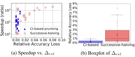
Since the two solutions are designed to satisfy different constraints (accuracy loss and resource), they are not directly comparable. We do our best to make a fair comparison. In this section, we run Successive-halving with identical sample size sequence as ABC, to compare the CI-based pruning and the halving strategy based on point estimation. We perform the same set of experiments as in the main experiment section for Successive-halving. We introduce a metric, calledrelative accuracy loss, to measure the difference between the returned configurationCi0and the best configurationC_i∗in terms of

the test accuracy: ∆rel = |Ai

∗−A_i0|

Ai∗ . The smaller∆rel is,

the better.

(a) Speedup vs.∆rel (b) Boxplot of∆rel

Figure 4: ABCvs. Successive-halving

We depict the comparison between Successive-halving and our ABCin Figure 4. The x-axis in Figure 4a refers to the relative accuracy loss compared to the best configuration by Full-run, y-axis is the speedup compared to the running time of Full-run, and each point corresponds to a specific experiment with a certain dataset andC. We can see that Successive-halving has a similar speedup as ABCover Full-run. However, the relative accuracy loss can be an order of magnitude larger than that of ABC, e.g.,8%vs.0.8%. This is because the pruning performed in Successive-halving is based on the ranking of the current test accuracy. On the contrary, ABCuses confidence interval of the real test accu-racy to perform safer pruning. Figure 4b presents a boxplot summarizing the relative accuracy loss for our solution and Successive-halving respectively. On average, the relative accuracy loss for our CI-based solution is0.24%(all below

1%), and 2% for Successive-halving (up to 8%), which is nearly ten times larger.

Related Work

frame-work, RoBO (Klein et al. 2017) treats the sample size as a hyperparameter, and uses random sample size to evaluate each configuration and a kernel function to extrapolate the real test accuracy.

Generalization Error Bounds.Generalization error bound has been studied extensively (Zhou 2002; Koltchinskii et al. 2000; Bousquet and Elisseeff 2002), among which VC-bound(Vapnik 1999) is a well-known technique for bounding the generalization error. The main idea behind VC-bounds is to useVC-dimensionto characterize the complexity of the hypothesis class. Besides VC-dimension, other existing tech-niques for deriving generalization error bounds include cover-ing number (Zhou 2002), Rademacher complexity (Koltchin-skii et al. 2000), and stability bound (Bousquet and Elisseeff 2002). While the definition of generalization error bounds is different from the confidence bound needed for ABC, they have been used in other work to guide progressive sampling for asingleconfiguration (Elomaa and K¨a¨ari¨ainen 2002).

Discussion and Conclusion

We studied the problem of efficiently finding approximate best configuration among a given set of training configura-tions for a large dataset. Our CI-based progressive sampling and pruning solution ABCcan successfully identify a top configuration with small or no accuracy loss, in much less time than the exact approach. The CI-based pruning is more robust than pruning based on point estimates.

There are multiple use cases that can benefit from our proposed ABC. The input of ABCcan be either specified by the users based on their domain knowledge, or generated from an AutoML search algorithm. Our ABCmodule can help data scientists identify a top configuration faster. As they iteratively refine it, they can use ABCto verify whether altering part of the configuration (such as changing features) boosts the performance, by invoking ABCwith the old and new configurations. In addition, our confidence bounds can be potentially used to accelerate Bayesian optimization and spectral search in large datasets, which is interesting future work.

References

Bergstra, J., and Bengio, Y. 2012. Random search for hyper-parameter optimization. Journal of Machine Learning Research

13(Feb):281–305.

Bergstra, J. S.; Bardenet, R.; Bengio, Y.; and K´egl, B. 2011. Al-gorithms for hyper-parameter optimization. InAdvances in neural information processing systems.

Bousquet, O., and Elisseeff, A. 2002. Stability and generalization.

Journal of machine learning research2(Mar):499–526.

Eggensperger, K.; Feurer, M.; Hutter, F.; Bergstra, J.; Snoek, J.; Hoos, H.; and Leyton-Brown, K. 2013. Towards an empirical foun-dation for assessing bayesian optimization of hyperparameters. In

NIPS workshop on Bayesian Optimization in Theory and Practice. Elomaa, T., and K¨a¨ari¨ainen, M. 2002. Progressive rademacher sampling. InAAAI’02, 140–145.

Feurer, M.; Klein, A.; Eggensperger, K.; Springenberg, J.; Blum, M.; and Hutter, F. 2015. Efficient and robust automated machine learning. InAdvances in Neural Information Processing Systems.

Hazan, E.; Klivans, A.; and Yuan, Y. 2018. Hyperparameter optimization: A spectral approach. InICLR’18.

Huang, S.; Wang, C.; Ding, B.; and Chaudhuri, S. 2018. Efficient identification of approximate best configuration of training in large datasets.arXiv preprint arXiv:1811.03250.

Hutter, F.; Hoos, H. H.; and Leyton-Brown, K. 2011. Sequential model-based optimization for general algorithm configuration. In

International Conference on Learning and Intelligent Optimization. Jamieson, K., and Talwalkar, A. 2016. Non-stochastic best arm iden-tification and hyperparameter optimization. InArtificial Intelligence and Statistics.

Klein, A.; Falkner, S.; Mansur, N.; and Hutter, F. 2017. Robo: A flexible and robust bayesian optimization framework in python. In

NIPS 2017 Bayesian Optimization Workshop.

Koltchinskii, V.; Abdallah, C. T.; Ariola, M.; Dorato, P.; and Panchenko, D. 2000. Improved sample complexity estimates for statistical learning control of uncertain systems.IEEE Transactions on Automatic Control45(12):2383–2388.

Li, L.; Jamieson, K.; DeSalvo, G.; Rostamizadeh, A.; and Tal-walkar, A. 2017. Hyperband: A novel bandit-based approach to hyperparameter optimization. InICLR’17.

Mund, S. 2015.Microsoft azure machine learning. Packt Publishing Ltd.

Olson, R. S.; Bartley, N.; Urbanowicz, R. J.; and Moore, J. H. 2016. Evaluation of a tree-based pipeline optimization tool for automat-ing data science. InProceedings of the Genetic and Evolutionary Computation Conference 2016, GECCO’16.

Pedregosa, F.; Varoquaux, G.; Gramfort, A.; Michel, V.; Thirion, B.; Grisel, O.; Blondel, M.; Prettenhofer, P.; Weiss, R.; Dubourg, V.; Vanderplas, J.; Passos, A.; Cournapeau, D.; Brucher, M.; Perrot, M.; and Duchesnay, E. 2011. Scikit-learn: Machine learning in python.

JMLR12:2825–2830.

Provost, F.; Jensen, D.; and Oates, T. 1999. Efficient progressive sampling. InACM SIGKDD international conference on Knowledge discovery and data mining.

Rasley, J.; He, Y.; Yan, F.; Ruwase, O.; and Fonseca, R. 2017. Hyperdrive: Exploring hyperparameters with pop scheduling. In

Proceedings of the 18th ACM/IFIP/USENIX Middleware Confer-ence, 1–13.

Sabharwal, A.; Samulowitz, H.; and Tesauro, G. 2016. Selecting near-optimal learners via incremental data allocation. InAAAI’16. Snoek, J.; Larochelle, H.; and Adams, R. P. 2012. Practical bayesian optimization of machine learning algorithms. InAdvances in neural information processing systems.

Sparks, E. R.; Talwalkar, A.; Haas, D.; Franklin, M. J.; Jordan, M. I.; and Kraska, T. 2015. Automating model search for large scale machine learning. InProceedings of the Sixth ACM Symposium on Cloud Computing.

Thornton, C.; Hutter, F.; Hoos, H. H.; and Leyton-Brown, K. 2013. Auto-weka: Combined selection and hyperparameter optimization of classification algorithms. InACM SIGKDD international confer-ence on Knowledge discovery and data mining.

Vanschoren, J.; van Rijn, J. N.; Bischl, B.; and Torgo, L. 2013. Openml: Networked science in machine learning.SIGKDD Explo-rations15(2):49–60.

Vapnik, V. N. 1999. An overview of statistical learning theory.

IEEE transactions on neural networks10(5):988–999.