The Thirty-Third AAAI Conference on Artificial Intelligence (AAAI-19)
Learning (from) Deep Hierarchical Structure among Features
Yu Zhang,
1Lei Han
2 1HKUST,2Tencent AI Lab[email protected], [email protected]
Abstract
Data features usually can be organized in a hierarchical struc-ture to reflect the relations among them. Most of previous studies that utilize the hierarchical structure to help improve the performance of supervised learning tasks can only han-dle the structure of a limited height such as 2. In this paper, we propose a Deep Hierarchical Structure (DHS) method to handle the hierarchical structure of an arbitrary height with a convex objective function. The DHS method relies on the ex-ponents of the edge weights in the hierarchical structure but the exponents need to be given by users or set to be identi-cal by default, which may be suboptimal. Based on the DHS method, we propose a variant to learn the exponents from data. Moreover, we consider a case where even the hierar-chical structure is not available. Based on the DHS method, we propose a Learning Deep Hierarchical Structure (LDHS) method which can learn the hierarchical structure via a gen-eralized fused-Lasso regularizer and a proposed sequential constraint. All the optimization problems are solved by prox-imal methods where each subproblem has an efficient solu-tion. Experiments on synthetic and real-world datasets show the effectiveness of the proposed methods.
Introduction
Most of previous studies to utilize the hierarchical struc-ture among feastruc-tures, including the group Lasso (Yuan and Lin 2006) and the Hierarchical Penalization (HP) method (Szafranski, Grandvalet, and Morizet-Mahoudeaux 2007), can only handle the hierarchical structure of a limited height up to 2. In this paper, we aim to break this assumption by utilizing the available hierarchical structure with an arbitrary height to help learn an accurate model. Moreover, in some case where the hierarchical structure is unavailable, we aim to learn such hierarchical structure among features to im-prove the interpretability of the resultant learner.
Specifically, given a hierarchical structure to describe re-lations among features, we propose a Deep Hierarchical Structure (DHS) method to utilize it. In the DHS method, each model parameter corresponding to a data feature is pe-nalized by the product of edge weights along the path from the root to the leaf node for that feature. Interestingly, when the exponents of the edge weights along the path from the
Copyright c2019, Association for the Advancement of Artificial Intelligence (www.aaai.org). All rights reserved.
root to each leaf node are summed to 1, the proposed ob-jective function can be proved to be convex no matter what the height of the hierarchical structure is. Moreover, when all the exponents take the same value, we can show that the proposed objective function is equivalent to a problem with a hierarchical group lasso regularization term. In order to optimize the objective function of the DHS method, we adopt the FISTA algorithm (Beck and Teboulle 2009) each of whose subproblems has an efficiently analytical solution. Moreover, in the proposed DHS method, the exponents of the edge weights need to be set based on a priori informa-tion. When this information is not available, by default we just set them to be identical. Usually this strategy works but it may be suboptimal. In order to alleviate this problem, we propose a variant of the DHS method to learn the exponents from data.
Moreover, we consider a more general case where the hi-erarchical structure is not available. A hihi-erarchical structure can give us more insight about the relations among features but learning it from data is a difficult problem. To the best of our knowledge, there is no work to directly learn the hier-archical structure among features. Here we give the first try based on the DHS method by proposing a Learning Deep Hierarchical Structure (LDHS) method. Given the height of the hierarchical structure, the LDHS method assumes that each path from the root to a leaf node corresponding to a data feature does not share any node between each other, then uses a generalized fused-Lasso regularizer to enforce nodes to fuse at each height, and finally designs a sequen-tial constraint to make the learned structure form a hierar-chical structure. For optimization, we use the GIST algo-rithm (Gong et al. 2013) to solve the objective function of the LDHS method. By comparing with several state-of-the-art baseline methods, experiments on several synthetic and real-world datasets show the effectiveness of the proposed models.
regres-sion, whose settings are different from ours. There are some methods (Bondell and Reich 2007; Hallac, Leskovec, and Boyd 2015; Figueiredo and Nowak 2016) which can learn the group structure among features but fail to learn the hier-archical structure, while the proposed LDHS method can do that.
NotationsA hierarchical structure is said to be balanced if the paths from the root to every leaf node have the same length. For unbalanced hierarchical structure, we can easily convert it to a balanced one by adding some internal nodes as shown in Figure 1. So in this paper, the hierarchical struc-ture mentioned is always assumed to be balanced. For a hi-erarchical structure of heightm, the root is at height0, the children of the root are at height1, and the leaf nodes are at heightm. The number of nodes at heightiis denoted bysi
and the nodes at heightiare labeled by1tosifrom left to
right. A node denoted byNi
j means that it is thejth node
at heighti. The set of children of a nodeNi
j is denoted by Ci
j and the number of children of a nodeNji is denoted by
d(ji). For each leaf nodeNm
i , we defined
(m)
i ≡ 1 for the
ease of the notations. We defineFi
j ≡kas the index of the
parent node ofNi
j, implying thatN i−1
k is the parent node of Ni
j. The edge from a nodeN i−1
j to one of its childrenN i k
is denoted byEj,k(i)and the weight of this edge is denoted by
σ(j,ki), where the superscript denotes the height in which the child node lies and the subscript denotes the indices of the parent and children nodes. The path from the root to theith leaf nodeNm
i is denoted by a sequence ofm+ 1integers
asPi ={i0, . . . , im}wherei0 = 1,im=i, and nodeN j ij is on the path forj = 0, . . . , m, and we definePij ≡ijas
the index of the node at heightjon the pathPi. In the
bot-tom figure of Figure 1, we haveC0
1 ={1,2,3},d (0)
1 = 3,
C1
2 = {3,4,5},d (1)
2 = 3,F
1
2 = 1, andF 2
3 = 2. The path
from the root to a leaf node N2
5 is P5 = {1,2,5} where
P0
5 = 1,P51= 2, andP52= 5.
Learning from Deep Hierarchical Structure
Most of the existing works such as the group Lasso and the HP method (Szafranski, Grandvalet, and Morizet-Mahoudeaux 2007) can only operate on a hierarchical struc-ture of a limited height. However, in many applications, the hierarchical structure is much more complex. To improve the applicability, we present the proposed DHS method in this section.
The Objective Function
Suppose the training dataset is denoted by D = {(xi, yi)}ni=1wherexi ∈ Rd denotes theith data instance andyiis its label, and the linear learning function is denoted
byf(x) =wTx. Suppose that the features are organized in
a balanced hierarchical structure of heightmwherem≥2. Based on a loss functionl(·,·,·), the objective function of
Figure 1: Illustration for the hierarchical structure. The top figure denotes a hierarchical structure and the bottom figure denotes the equivalently balanced structure.
the DHS method is formulated as
min
w,σ
1 n
n
X
i=1
l(xi, yi,w) +
λ1
2
d
X
i=1
w2 i
Qm j=1
σ(j)
Pij−1,Pji θ(j)
Pij−1,Pij
+λ2 2 kwk
2 2
s.t.
si X
j=1
d(ji)σ(Fi)i j,j
= 1∀i∈[m], σF(i)i j,j
≥0∀i, j, (1)
wherewiis theith entry inw, an edge weightσ
(j)
c,dis defined
in the previous section,k·k2denotes the`2norm of a vector,
a/bfor two scalarsaandbis defined by continuation at zero asa/0 =∞ifa6= 0and0/0 = 0,[m]denotes an integer set from 1 tom, andθ(j)
Pj−1 i ,P
j i
, an exponent, can be viewed as
the importance for the edge weightσ(j)
Pj−1 i ,P
j i
. The summand
in the second term of the objective function in problem (1) penalizes eachwi based on all the weights of edges on the
path from the root node to theith leaf node as well as the ex-ponents. Hence two coefficientswiandwjwill tend to have
similar penalizations if they share many edges in the hierar-chical structure. As we will see in Theorem 3, when expo-nents are identical to each other, this term is related to the group Lasso regularizer which enforces the group sparsity. The equality constraint in problem (1) is to restrict the scale of σ. To preserve the convexity of problem (1) as we will see in the next section, it is required thatθ(j)
Pij−1,Pij ≥0∀i, j andPm
j=1θ (j)
Properties
We first introduce a new family of convex functions with the proof in the supplementary material.
Theorem 1 f(w,z) = Qmw2
i=1zθii
is jointly convex with
re-spect to w ∈ R and z = (z1, . . . , zm)T ∈ Rm, where
zi’s are required to be positive, given that θi ≥ 0 for
i= 1, . . . , mandPm
i=1θi= 1.
Whenm= 1, Theorem 1 asserts thatf(w, z) =w2/zis jointly convex with respect towandzwhenz >0, which is a well-known result (pp. 72, (Boyd and Vandenberghe 2004)). Whenm= 2andθ1=θ2= 1/2, Theorem 1
recov-ers Proposition 1 in (Szafranski, Grandvalet, and Morizet-Mahoudeaux 2007). Theorem 1 is more general sincemcan be any positive integer and differentθi’s can have different
values.
Based on Theorem 1, we can prove the convexity of prob-lem (1) in the following theorem.
Theorem 2 Given that the loss functionl(x, y,w)is convex withw, problem (1) is jointly convex with respect towand σ.
To see the effect of the regularizer in the second term of problem (1), we investigate two special cases, where
m equals 2 or 3. When m = 2, problem (1) degen-erates to the HP method (Szafranski, Grandvalet, and Morizet-Mahoudeaux 2007), which shows that when all the
θ(j)
Pij−1,Pij’s equal 1
2, problem (1) is equivalent to the `43,1 -regularized group Lasso. Whenm = 3, we can derive an equivalent formulation of problem (1) as follows.
Theorem 3 Whenm = 3and all the θ(j)
Pj−1 i ,P
j i
’s equal 13,
problem (1) is equivalent to this problem:
min w λ1 2 s1 X i=1
(d(1)i )16
X
j∈C1 i
(d(2)j )15
X
k∈C2 j
|wk|32 4 5 5 6 2 + 1 n n X i=1
l(xi, yi,w) +
λ2
2 kwk
2
2. (2)
According to Theorem 3, we can see the second term in the objective function of problem (1) can be converted to the first one of problem (2), which places the`3
2 norm on model parameters corresponding to the leaf nodes which share the same parent node, then places the weighted`6
5 norm on the internal nodes at height 2 which have the same parent node, and finally computes the squared weighted sum on the in-ternal nodes at height 1. This regularizer can be viewed as a hierarchical group Lasso where at each height, the weights corresponding to nodes sharing the same parent node will be combined together via some norm. In general, for any posi-tive integerm, when all the exponents of differentσij,khave the same value (i.e.,1/m), we can always find the explicit form of the second term in the objective function of problem (1) in a similar way to the proof of Theorem 3.
Optimization
Since problem (1) is convex, we use the FISTA method (Beck and Teboulle 2009) to solve it. We use a variableφ to denote the concatenation ofwandσ. We define
f(φ) =
n
X
i=1
l(xi, yi,w)
n +
d
X
i=1
λ1w2i
2Qm j=1
σ(j)
Pji−1,Pij θ(j)
Pji−1,Pij
andg(φ) =λ2
2kwk 2
2. We define the set of constraints onφ
as
Sφ={φ| si X
j=1
d(ji)σ(Fi)i j,j
= 1∀i∈[m], σF(i)i j,j
≥0∀i, j}.
In the FISTA algorithm, it does not minimize the original composite objective functionF(φ) =f(φ) +g(φ), but in-stead solves a surrogate function:
qr(φˆ) = arg min φ∈Sφ
Qr(φ,φˆ),
whereQr(φ,φˆ) =g(φ) +f(φˆ) + (φ−φˆ)T 5φf(φˆ) + r
2kφ−φˆk 2
2and5φf(φˆ)denotes the derivative off(φ)with
respect toφatφ=φˆ. Hence, in the FISTA algorithm, we just need to minimize Qr(φ,φˆ)with respect toφ ∈ Sφ.
Specifically, we need to solve the following problem:
min
w,σ
λ2
2 kwk
2
2+
r
2kw−w˜k
2
2+
r
2kσ−σ˜k
2 2
s.t.
si X
j=1
d(ji)σ(Fi)i j,j
= 1∀i∈[m], σF(i)i j,j
≥0∀i, j, (3)
whereris a step size which can be determined by the FISTA algorithm,w˜=wˆ−1
r5wf(wˆ), andσ˜=σˆ−
1
r5σf(σˆ).
It is easy to see that the solution for w in problem (3) is
w = r
λ2+rw˜. For σ in problem (3), we can find that the corresponding problem can be decomposed intom−1 sub-problems with each one solving a problem with respect to
{σ(i)
Fi j,j
}si
j=1 and these subproblems have the same
formula-tion as
min
ρ kρ−ρˆk
2
2 s.t. ρ≥0, aTρ= 1, (4)
where0denotes a zero vector with appropriate size,≥ de-notes the elementwise inequalities between two vectors, and ais a constant vector with all entries positive. Problem (4) is a quadratic programming (QP) problem and we can use some off-the-shelf QP solver to solve it. To accelerate the optimization of problem (4), we propose a more efficient solution for problem (4) by solving its dual form and the detailed procedure is put in the supplementary material.
A Variant to Learn Exponents
In the DHS method, we need to manually set the expo-nents {θ(j)
Pj−1 i ,P
j i
}. By default, we usually assume that all
the θ(j)
Pj−1 i ,P
j i
’s are equal to m1, which satisfies the
this setting may be suboptimal. In this section, we propose a DHSemethod, a variant of the DHS method, to learn the
exponents from data directly.
The objective function of the DHSemethod is formulated
as
min
w,σ,θ
1 n
n
X
i=1
l(xi, yi,w) +
λ1 2 d X i=1 w2 i Qm j=1
σ(j)
Pji−1,Pij θ(j)
Pij−1,Pij
+λ2 2 kwk
2 2 s.t. si X j=1
d(ji)σ(i)
Fi j,j
= 1∀i∈[m], σ(i)
Fi j,j
≥0∀i, j
m
X
j=1
θ(j)
Pj−1
i ,P j i
= 1∀i∈[d], θ(j)
Pj−1
i ,P j i
≥0∀i, j. (5)
Different from problem (1) where all the θ(j)
Pj−1 i ,P
j i
’s are
constants, all the θ(j)
Pj−1 i ,P
j i
’s in problem (5) are variables
to be optimized. The equality and inequality constraints with respect to θ in problem (5) satisfy the requirements for the constant exponents in problem (1) and they form an(m−1)−dimensional simplex for each feature. Differ-ent from problem (1) which is convex, problem (5) can be proved to be non-convex with respect to all variables and hence we use the GIST algorithm (Gong et al. 2013) to solve it. Due to page limit, we put the detailed optimization pro-cedure in the supplementary material.
Learning Deep Hierarchical Structure
In some applications, the hierarchical structure is not avail-able. In this section, we propose the LDHS method to learn both the hierarchical structure and the model parameters from data directly.
We assume that the height of the hierarchical structure to be learned is given as m. Here we use slightly dif-ferent notations to define the hierarchical structure. The weights of edges on the path from the root node to theith leaf node corresponding to the ith feature are denoted by
{ω(1)i , . . . , ωi(m)}, whereωi(j)denotes the weight of an edge connecting the heightj−1andjon the path from the root node to theith leaf node. At the beginning, we assume that the paths from the root node to any two different leaf nodes do not share any edge. Whenω(ji)equalsω(ki)for somei,j
andk, we can view it as a sign for that the two paths from the root node to thejth andkth leaf nodes become fused at heightiand then in order to keep the whole structure as a hi-erarchical structure, it should be required that the subpaths on the two paths above heightiare always fused, implying
that ω(ji0) will always equal ωk(i0) when i0 ≤ i. So an al-gorithm that can learn a valid hierarchical structure should satisfy the following two requirements:
(1) It should have the ability to enforceωj(i)to be equal to
ωk(i)for somei,jandk;
(2) It should guarantee that when ωj(i) equalsω(ki), for all
i0< i,ω(i
0)
j will equalω
(i0)
k .
Here we present the objective function of the LDHS method which can satisfy those two requirements:
min
w,ω
1 n
n X
i=1
l(xi, yi,w) +
λ1 2 d X i=1 w2 i Qm j=1
ωi(j)
1 m
+λ2 2 kwk
2 2+ m X i=1 ηi X j<k
|ω(ki)−ωj(i)|
s.t.
d X
j=1
ωj(i)= 1∀i∈[m], ωj(i)≥0∀i, j
|ω(1)k −ωj(1)| ≤. . .≤ |ωk(m)−ωj(m)| ∀j, k, (6)
where ω is a vector containing all ωi(j)’s. The last term in the objective function of problem (6), a layer-wise gen-eralized fused-Lasso regularizer (Tibshirani et al. 2005; Hocking et al. 2011), can makeω(ji)equal toωk(i)for somei,
j andk, and so this regularizer can satisfy the first require-ment. The sequential inequality constraint in problem (6) can satisfy the second requirement since when ω(ji) equals
ω(ki), we can get |ω(i
0)
j −ω
(i0)
k | ≤ 0 for any1 ≤ i
0 < i,
implying thatωj(i0) =ω(ki0). Therefore, problem (6), which satisfies the two requirements, can learn a hierarchical struc-ture. The exponents of all theω(ij)’s are set to bem1. We can also set them to be other values or even learn them as the DHSe method did and this will be left as the future work.
The regularization parameterηicontrols the level of fusion
between{ω(ji)}d
j=1at heighti. A largerηiwill lead to more
identical values in{ω(ji)}d
j=1. Therefore, it is intuitive to
de-fine an increasing order forηi’s from heightmto height 0
to help construct the hierarchical structure. In practice, we set ηi−1 = υηi for i ≥ 2 with some constant υ > 1.
When the hierarchical structure is available or equivalently ωis given, problem (6) becomes problem (1) and hence the LDHS method is a generalization of the DHS method to learn the hierarchical structure.
Even though the objective function of problem (6) is con-vex based on Theorem 1, the whole problem is non-concon-vex due to the sequential inequality constraint and we also use the GIST method to solve it. We still use the variableφto denote the concatenation ofwandω. We define a set of con-straints onφasSφ={φ|Pd
j=1ω (i)
j = 1∀i∈[m], ω
(i)
j ≥ 0∀i, j, |ω(1)k −ωj(1)| ≤ . . . ≤ |ωk(m)−ω(jm)| ∀j, k.}. We define
g(φ) =
(
λ2kwk22
2 +
Pm
i=1ηiPj<k|ω (i) k −ω
(i)
j | ifφ∈ Sφ
+∞, otherwise
f(φ) =1 n
n
X
i=1
l(xi, yi,w) +
λ1
2
d
X
i=1
w2i
Qm j=1
ωi(j)
1 m
.
be solved in the GIST algorithm can be formulated as
min
w,ω
r
2kw−w˜k
2
2+
r
2kω−ω˜k
2
2+
λ2
2 kwk
2 2
+ m X
i=1
ηi X
j<k
|ωk(i)−ωj(i)|
s.t.
d X
j=1
ωj(i)= 1∀i∈[m], ω(ji)≥0∀i, j
|ω(1)k −ω(1)j | ≤. . .≤ |ωk(m)−ωj(m)| ∀j, k, (7)
wherewˆ andωˆ are previous estimations for w andω re-spectively,w˜ =wˆ−1
r5wf(wˆ), andω˜=ωˆ−
1
r5ωf(ωˆ).
It is easy to see that the solution for w in problem (7) is
w= r
λ2+rw˜. Forωin problem (7), its problem can be sim-plified as
min
ω
r
2kω−ω˜k
2
2+
m X
i=1
ηikBω(i)k1 (8)
s.t.1Tω(i)= 1, ω(i)≥0, |Bω(1)| ≤. . .≤ |Bω(m)|,
where k · k1 denotes the `1 norm of a vector, ω(i) =
(ω1(i), . . . , ωd(i))T,1is a vector of all ones with an
appro-priate size,|a|for a vectorareturns a vector with each entry being the absolute value of the corresponding entry ina,≥
denotes the elementwise “no smaller than” relation between two vectors, andBis a d(d2−1) ×dmatrix with each of its rows containing only two non-zero entries1and−1at corre-sponding locations. Problem (8) seems complicated and we reformulate it as
min
ω,µ,τ
r
2kω−ω˜k
2
2+
m X
i=1
ηikτ(i)k1
s.t.1Tω(i)= 1,ω(i)≥0,µ(i)=ω(i),τ(i)=Bµ(i)
|τ(1)| ≤. . .≤ |τ(m)|. (9) Due to the existent of linear equality constraints, we use the ADMM to solve problem (9). We define the augmented La-grangian function as
L(ω,µ,τ)
= m X
i=1
ρ
2kτ
(i)−Bµ(i)k2
2+q
T i(τ
(i)−Bµ(i))
+ m X
i=1
pTi (µ(i)−ω(i)) +ρ 2kµ
(i)−ω(i)k2 2
+r
2kω−ω˜k
2
2+
m X
i=1
ηikτ(i)k1,
where{pi}m
i=1 and{qi}mi=1 act as Lagrangian multipliers,
andρis a penalty parameter. Then we need to solve the fol-lowing problem as
min
ω,µ,τ L(ω,µ,τ)
s.t.1Tω(i)= 1, ω(i)≥0∀i∈[m]
|τ(1)| ≤. . .≤ |τ(m)|. (10)
In the ADMM algorithm, problem (10) can be solved alter-natively with respect toω,µandτ.
With fixedµandτ, we need to solve the following sub-problem with respect toωas:
min
ω m X
i=1
kω(i)−b(i)k2 2 s.t.1
Tω(i)= 1, ω(i)≥0∀i,
whereb(i) = 1
r+ρ rω˜
(i)+p
i+ρµ(i). This problem can
be decomposed intomsubproblems where theith subprob-lem with respect toω(i)has the same formulation as
prob-lem (4), which has an efficient solution.
With fixedωandτ, the subproblem with respect toµis a QP problem. By setting the derivative ofL(ω,µ,τ)with respect toµ(i)to zero, we can obtain the analytical solution
forµ(i)as
µ(i)= I+BTB−1
BTτ(i)+1 ρB
Tq
i+ω(i)−
1 ρpi
.
Note that (I+BTB)−1 is a constant matrix. So it can
be computed and stored before solving the whole problem, leading to a more efficient implementation.
With fixedωandµ, the subproblem with respect toτcan be decomposed into 12d(d−1)subproblems with thejth one formulated as
min
τ(i)
m X
i=1
ρ 2
τj(i)−νj(i)
2
+ηi|τj(i)|
s.t. |τj(1)| ≤. . .≤ |τj(m)|, (11)
whereν(i)=Bµ(i)−1
ρqiandτ
(i)
j ,ν
(i)
j are thejth entries
ofτ(i)andν(i), respectively. The optimalτ(i)
j must have the
same sign asνj(i)since otherwise we can flip the sign ofτj(i)
to achieve a lower value for the first term in the summand of the objective function in problem (11) while keeping other terms unchanged and also satisfying the constraints, which leads to a lower objective value. Then by defining new vari-ables{τˆj(i)}asτˆj(i) = sgn(νj(i))τj(i)wheresgn(·)gives the
sign of a scalar, τˆj(i) is always nonnegative and based on
problem (11), the problem with respect to{τˆj(i)}can be for-mulated as
min
{τˆj(i)}
m X
i=1
ˆ
τj(i)−νˆj(i)
2
s.t.0≤ˆτj(1)≤. . .≤τˆj(m), (12)
whereνˆj(i)=|νj(i)|−1
ρηi. This problem is similar to problem
(17) in (Han and Zhang 2015b) except the requirement that all τˆj(i)’s are nonnegative. We first use the algorithm with linear complexity in Section 3.2 of (Han and Zhang 2015b) to solve this problem and then make negative ones in{τˆj(i)}
become zero to obtain the final solution.
Experiments
We compare the proposed models (i.e., DHS, DHSe
and LDHS) with state-of-the-art structured feature learning methods, including the Lasso, Group Lasso (GLasso) (Yuan and Lin 2006), the CAP family with`4and`∞penalties de-noted by CAP`4 and CAP`∞ (Zhao, Rocha, and Yu 2009), and the HP method (Szafranski, Grandvalet, and Morizet-Mahoudeaux 2007). Among these baseline methods, the Lasso method does not take any group or hierarchical struc-ture into consideration and the GLasso and HP models re-quire a hierarchical structure of height 2, while the CAP, DHS and DHSemethods need a hierarchical structure with
an arbitrary height. In order to provide a fair comparison, in all the experiments we first generate a hierarchical struc-ture on the feastruc-tures and then apply it to the GLasso, CAP, HP, DHS and DHSemethods, where the group structure
re-quired by the GLasso and HP methods is obtained from the two bottom-most layers of the hierarchical structure. For the LDHS method, we set its height to be that of the given hier-archical structure.
Experiments on Synthetic Data
We first experiment on synthetic data. We generate three synthetic data by varying the height of the hierarchical struc-ture as m = 3,4 and 5, respectively. For simplicity, we use full binary trees and the numbers of features d under the three settings are equal to23,24 and25, respectively.
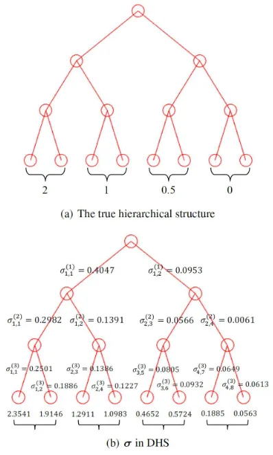
The ground truth of the feature weightsw∗whenm= 3is shown in Fig. 2(a) and those for other cases are put in the supplementary material. Then, we generate data instances from a normal distribution N(0,Id), where Id is ad×d
identity matrix. We assume a linear model between data in-stances and labels, i.e.,y=Xw∗+with each entryiin (i = 1,· · · , n) followingN(0, ξ2). In all the settings, we
generaten= 100training samples and setξ= 2.
Table 1: The MSE’s in terms of ‘mean±std’ on synthetic data.
m= 3 m= 4 m= 5
Lasso 0.2913±0.0399 0.8669±0.0499 1.8660±0.0549 GLasso 0.2945±0.0372 0.8597±0.0402 1.8877±0.0593 CAP`4 0.3069±0.0349 0.8597±0.0402 1.8885±0.0495
CAP`∞ 0.3069±0.0349 0.8597±0.0402 1.8886±0.0497
HP 0.2795±0.0439 0.8403±0.0314 1.5519±0.0550 DHS 0.2743±0.0337 0.8275±0.0336 1.4682±0.0433 DHSe 0.2748±0.0305 0.8337±0.0324 1.5596±0.0474
LDHS 0.2370±0.0303 0.8283±0.0354 1.3894±0.0460
We randomly generate 100 samples for testing and use another100 random samples for validation to choose reg-ularization parameters of all the methods. All of the regu-larization parameters in different models are chosen from a set{10−5,10−4· · · ,1}, exceptηi’s in the proposed LDHS
method. As discussed before, we setηi+1=ηi/υfori < m,
where we chooseη1 andυ from {10−5,10−4· · ·,1} and
{1.1,2,10}, respectively. We use the Mean Square Error (MSE) to evaluate different methods, where the MSE is de-fined as 1n( ˆw−w∗)>X>X( ˆw−w∗)for an estimationwˆ. All the settings are repeated for 10 times to obtain the av-erage results, which are reported in Table 1. From the results,
Figure 2: The true hierarchical structure and estimated pa-rameters whenm= 3.
we observe that the proposed models with deeper hierarchi-cal structure, i.e., the DHS, DHSeand LDHS models,
gen-erally show better performance than Lasso, GLasso, CAP`4, CAP`∞ and HP. This demonstrates that whenever features can be organized into a deeper hierarchical structure, using the correct (deeper) hierarchical structure will allow a lower prediction error compared to models with shallow struc-ture, e.g., groups or a hierarchical structure of height 2. The GLasso, CAP`4 and CAP`∞ methods show comparable re-sults since all of them belong to the CAP family and may ac-quire similar information from the feature groups. The DHS and DHSe methods show comparable performance, while
the LDHS method, which learns the hierarchical structure automatically, achieves the lowest MSE in two of all the three settings.
Moreover, in Fig. 2, we show the estimated parameter σ in the DHS method and ω in the LDHS method when
m= 3. The estimatedσin DHSeis similar to that in DHS,
Table 2: The MSE’s (in terms of ‘mean±std’) of different methods on the Traffic Volume data.
Task 1 Task 2 Task 3 Task 4 Task 5
Lasso 0.1066±0.0179 0.1366±0.0279 0.1155±0.0231 0.1215±0.0132 0.1632±0.0352 GLasso 0.1042±0.0190 0.1185±0.0201 0.1030±0.0228 0.0934±0.0122 0.1725±0.0264 CAP`4 0.0939±0.0173 0.1122±0.0164 0.0944±0.0180 0.0864±0.0109 0.1609±0.0251 CAP`∞ 0.0977±0.0172 0.1179±0.0222 0.1029±0.0193 0.0925±0.0136 0.1800±0.0223 HP 0.0869±0.0189 0.1087±0.0270 0.0963±0.0196 0.0915±0.0133 0.1403±0.0299 DHS 0.0839±0.0187 0.1049±0.0262 0.0929±0.0187 0.0884±0.0132 0.1374±0.0284 DHSe 0.0843±0.0189 0.1051±0.0262 0.0935±0.0189 0.0890±0.0128 0.1381±0.0290
LDHS 0.0838±0.0186 0.1048±0.0262 0.0928±0.0186 0.0882±0.0126 0.1373±0.0284
well matches the hierarchical structure. For example, the es-timatedσ along the path from the root to the last four fea-tures are generally small. According to the formulation of the DHS model, theseσ’s will give heavier penalizations on the corresponding feature weights and as a consequence, we can obtain small feature weights, which match the true val-ues ofw∗. Similarly, for the LDHS model, the parameterω is anm×dmatrix. We show the estimatedωin Fig. 2(c), from which we can generally observe a hierarchical ture by comparing their values, and this hierarchical struc-ture well matches the ground truth. This result demonstrates that the LDHS method is able to recover the hierarchical structure.
Experiments on Real-World Datasets
In this section, we experiment on three real-world datasets including the traffic volume data (Han and Zhang 2015b), the breast cancer data (Jacob, Obozinski, and Vert 2009) and the Covtype data. In these datasets, the hierarchical structure over the features is not available. By following (Kim and Xing 2010), we use a simple hierarchicalk-means cluster-ing method to generate the hierarchical structure on the fea-tures. Specifically, we perform k-means clustering to split the features into two groups, and for each group we recur-sively performk-means clustering to obtain four sub-groups. Therefore, the resultant hierarchical structure has a height of
m = 3and hence in the LDHS method, the height of the learned hierarchical structure is also set to 3. The following experiments show that such a simple hierarchical structure is sufficient to obtain good performance for the proposed methods.
First we experiment on the traffic volume data. This dataset collects the traffic volumes from 136 entries (treated as features) and the traffic volumes through some exits (treated as response) in a highway traffic network. We choose 5 exits with the highest volumes in the network to form 5 learning tasks, each of which is to use the volumes from entries to predict the volume through a specific exit. There are totally 384 data samples. These tasks are regres-sion problems and we use the square loss for all the meth-ods. We randomly select 80% and 20% samples for train-ing and testtrain-ing, respectively. The regularization parameters are chosen from the same candidate set as used in the syn-thetic setting via 5-fold cross-validation. We use the MSE, i.e.,n1ky−yˆk2
2, to measure the performance of all the
meth-ods. The results on the 5 tasks are given in Table 2. From the
results, we observe that in 4 out of the 5 tasks, the proposed DHS, DHSe and LDHS methods outperform the baseline
methods and the LDHS method achieves the lowest MSE. This demonstrates again that a deeper tree structure can pro-vide a better feature structure in this data and our proposed methods can take advantage of this structure.
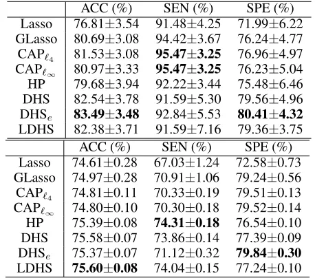
Table 3: Results on the Breast Cancer (top) and Covtype (bottom) datasets.
ACC (%) SEN (%) SPE (%)
Lasso 76.81±3.54 91.48±4.25 71.99±6.22 GLasso 80.69±3.08 94.42±3.67 76.24±4.77 CAP`4 81.53±3.08 95.47±3.25 76.96±4.97 CAP`∞ 80.97±3.33 95.47±3.25 76.23±5.04 HP 79.68±3.94 92.22±3.44 75.48±6.46 DHS 82.54±3.78 91.59±5.30 79.56±4.96 DHSe 83.49±3.48 92.84±5.53 80.41±4.32
LDHS 82.38±3.71 91.59±7.16 79.36±3.75
ACC (%) SEN (%) SPE (%)
Lasso 74.61±0.28 67.03±1.24 72.58±0.73 GLasso 74.97±0.28 70.91±1.06 79.24±0.56 CAP`4 74.81±0.11 70.33±0.19 79.51±0.13 CAP`∞ 74.80±0.10 70.30±0.18 79.52±0.14 HP 75.39±0.08 74.31±0.18 76.54±0.10 DHS 75.58±0.07 73.86±0.14 77.39±0.09 DHSe 75.37±0.07 71.12±0.32 79.84±0.30
LDHS 75.60±0.08 74.04±0.15 77.24±0.10
feature dimensionality isd= 54. We evaluate all the meth-ods on these two datasets based on three mesuares, i.e., the accuracy (ACC), sensitivity (SEN), and specificity (SPE), similar to (Yang et al. 2012; Han and Zhang 2015a). By following (Yang et al. 2012; Han and Zhang 2015a), 50%, 30% and 20% of the data are randomly chosen for train-ing, validation, and testtrain-ing, respectively. The regularization parameters are selected from the same candidate sets as de-scribed in the previous experiments. The top table in Table 3 shows the average results over 10 repetitions on the breast cancer data. According to the results, hierarchical methods with deep tree structure generally show more accurate pre-dictions. The DHSemethod achieves the best performance
in this case. The CAP`4and CAP`∞have better sensitivities than the proposed methods, implying that they can recover more true positive examples, while their SPE is lower. Ac-cording to results reported in the bottom table of Table 3, we can see that the HP, DHS, DHSe, and LDHS generally
outperform the Lasso and GLasso methods on the Covtype data. Again, the LDHS method, which learns the tree struc-ture, obtains the best accuracy.
Conclusions
In this paper, we study the problem of learning (from) deep hierarchical structure step by step. In the first step, we pro-pose the convex DHS method to learn from hierarchical structure with an arbitrary height. Secondly, we propose the DHSemethod, a variant of the DHS method, to learn the
ex-ponents from data. Finally, we propose the LDHS method to learn the hierarchical structure since it may be unavailable in some applications.
In our future work, we will learn the exponents of the LDHS method in a way similar to the DHSemethod.
Acknowledgment
This research has been supported by NSFC (61473087 and 61673202).
References
Beck, A., and Teboulle, M. 2009. A fast iterative shrinkage-thresholding algorithm for linear inverse problems. SIAM Journal on Imaging Sciences2(1):183–202.
Bondell, H., and Reich, B. 2007. Simultaneous regression shrinkage, variable selection, and supervised clustering of predictors with OSCAR. Biometrics64:115–123.
Boyd, S., and Vandenberghe, L. 2004.Convex Optimization. New York, NY: Cambridge University Press.
Chang, C.-C., and Lin, C.-J. 2011. LIBSVM: A library for support vector machines. ACM Transactions on Intelligent Systems and Technology2(3):27.
Figueiredo, M. A. T., and Nowak, R. D. 2016. Ordered weighted L1 regularized regression with strongly corre-lated covariates: Theoretical aspects. InProceedings of the 19th International Conference on Artificial Intelligence and Statistics, 930–938.
Gong, P.; Zhang, C.; Lu, Z.; Huang, J.; and Ye, J. 2013. A general iterative shrinkage and thresholding algorithm
for non-convex regularized optimization problems. In Pro-ceedings of the 30th International Conference on Machine Learning, 37–45.
Hallac, D.; Leskovec, J.; and Boyd, S. P. 2015. Network lasso: Clustering and optimization in large graphs. In Pro-ceedings of the 21th ACM SIGKDD International Confer-ence on Knowledge Discovery and Data Mining, 387–396. Han, L., and Zhang, Y. 2015a. Discriminative feature group-ing. InProceedings of the 29th AAAI Conference on Artifi-cial Intelligence.
Han, L., and Zhang, Y. 2015b. Learning tree structure in multi-task learning. In Proceedings of the 21st ACM SIGKDD Conference on Knowledge Discovery and Data Mining.
Hocking, T.; Vert, J.-P.; Bach, F.; and Joulin, A. 2011. Clus-terpath: An algorithm for clustering using convex fusion penalties. InProceedings of the 28th International Confer-ence on Machine Learning, 745–752.
Jacob, L.; Obozinski, G.; and Vert, J.-P. 2009. Group lasso with overlap and graph lasso. In Proceedings of the 26th International Conference on Machine Learning, 433–440. Kim, S., and Xing, E. P. 2010. Tree-guided group lasso for multi-task regression with structured sparsity. In Pro-ceedings of the 27th International Conference on Machine Learning, 543–550.
Szafranski, M.; Grandvalet, Y.; and Morizet-Mahoudeaux, P. 2007. Hierarchical penalization. In Platt, J. C.; Koller, D.; Singer, Y.; and Roweis, S. T., eds.,Advances in Neural Information Processing Systems 20, 1457–1464.
Tibshirani, R.; Saunders, M.; Rosset, S.; Zhu, J.; and Knight, K. 2005. Sparsity and smoothness via the fused lasso. Jour-nal of the Royal Statistical Society Series B67(1):91–108. Yang, S.; Yuan, L.; Lai, Y.-C.; Shen, X.; Wonka, P.; and Ye, J. 2012. Feature grouping and selection over an undirected graph. InProceedings of the 18th ACM SIGKDD Confer-ence on Knowledge Discovery and Data Mining, 922–930. Yuan, M., and Lin, Y. 2006. Model selection and estima-tion in regression with grouped variables. Journal of the Royal Statistical Society: Series B (Statistical Methodology) 68(1):49–67.