Privacy Law
Volume 2
Issue 1
Computer/Law Journal - 1980
Article 29
1980
Mathematical Models For Legal Prediction, 2
Computer L.J. 829 (1980)
R. Keown
Follow this and additional works at:
http://repository.jmls.edu/jitpl
Part of the
Computer Law Commons
,
Internet Law Commons
,
Privacy Law Commons
, and the
Science and Technology Law Commons
http://repository.jmls.edu/jitpl/vol2/iss1/29
This Article is brought to you for free and open access by The John Marshall Institutional Repository. It has been accepted for inclusion in The John Marshall Journal of Information Technology & Privacy Law by an authorized administrator of The John Marshall Institutional Repository.
Recommended Citation
MATHEMATICAL MODELS FOR
LEGAL PREDICTION
by
R.
KEOWN*INTRODUCTION
This article discusses some ideas concerning the prediction of judicial decisions by means of mathematical models. In a recent ar-ticle, Mackaay and Robillard developed the "nearest neighbour rule" and collected a number of references to schemes predicting the out-comes of cases presented to a judicial body for decision.1 Their pa-per credits Kort with the initial effort in this field.2 Besides their own method of nearest neighbours, the two authors discuss proce-dures of McCarthy employing ideas from the theory of "artificial in-telligence" to develop logical methods of case analysis and prediction,3 various approaches of Lawlor concerning linear predic-tion schemes,4 and review work of others-a description of whose
efforts will not be attempted here.
This article begins with the method of linear models, goes on to that of catastrophic models, and concludes with the scheme of
near-est neighbours. Unfortunately, the concepts required for a full un-derstanding of catastrophe theory do not form a part of the standard equipment of most professional mathematicians, much less that of most practicing attorneys, so that this article must be directed pri-marily toward exhibiting the general flavor of the subject, rather
* B.S. physics 1946, University of Texas; Ph.D. mathematics 1950, Massachusetts Institute of Technology; candidate for J.D. 1981, University of Arkansas. Since 1967, Dr. Keown has been a professor of mathematics at the University of Arkansas, Fay-etteville, Arkansas.
1. Mackaay & Robillard, Predicting Judicial Decisions: The Nearest Neighbour
Rule and Visual Representation of Case Patterns, 3 DATENVERARBErrUNG i REcHT 47 (1974).
2. Kort, Predicting the Supreme Court Decisions Mathematically: a Qualitative
Analysis of the "Right-to-Counsel" Cases, 51 Am. PoL ScI. REV. 1 (1957).
3. McCarthy, Reflections on Taxman: An Experiment in Artificial Intelligence
and Legal Reasoning, 90 HiARv. I. REV. 837 (1977).
4. Lawlor, What Computers Can Do: Analysis and Prediction of Judicial Deci.
than toward a penetrating analysis. In this regard, Zeeman gives one of the most satisfactory presentations of the basic ideas for non-mathematical readers.5 Recently Behavioral Science devoted an en-tire issue to applications of catastrophe theory in the behavioral and life sciences, including a critique by two well-known detractors, Sussman and Zahler.6 With these difficulties in view, it may be worthwhile to note that since the technique of linear programming has been widely introduced during the past twenty-five years, the notion of a general linear equation is understood by a much wider audience than ever before. Consequently, an effort will be made to describe some of the fundamental objects of catastrophe theory through the agency of linear models.
Before beginning with these models, it is necessary to introduce a few geometric concepts in an algebraic setting. Doubtless, these will be too elementary for some and too distracting for others. Nev-ertheless, some sort of an introduction is required to this complex of ideas and notation. Two of the basic notions of geometric analysis are that of a plane P corsisting of all the ordered pairs (x, y) where x and y are real numbers and that of a line L, which is the set "{(x,
y): ax + by + c = 0 for some numbers, a, b, and c}." This last "{ : }" is standard mathematical notation for a set S = (x: p(x)) consisting of all objects x where x is an object with property p. For example, J = {x: x is a federal judge) denotes the set of all federal judges; D = (x:
x is a defendant in a California court during 1978) is the set of all defendants which appeared in California courts during 1978; and S = {x: x is a rule in the Income Tax Regulations of 1977) is the set of all rules which appear in the Income Tax Regulations of 1977.
The concepts of plane and line are geometrical in that they are geometric ideas historically as well as in the sense that meaningful pictures can be drawn of them. These are as follows:
5. E. ZIEMAN, CATASTROPHE THEORY: SELECTED PAPERS (1972-1977)(1977).
6. Sussman & Zahler, A Critique of Applied Catastrophe Theory in the
1980]MATHEMATICAL MODELS FOR LEGAL PREDICTION 831
Y Y
(0 11
(0)1
\2 (1 0)
(-1 ,0)1
0--(0,0) (0)0) X
(i)
(ii)
FIGURE 1
Figure l(i) is a "picture" of the so-called x, y-plane containing the line L1 of all points with coordinates (x, y) which satisfy the
equa-tion x - y + 1 = 0, while Figure 1 (ii) is the "same plane" containing
the line L2. Intuitively the plane is a two-dimensional object while
the embedded line is a one-dimensional object.
Such intuitive concepts of dimension can be given forbiddingly mathematical definitions and, based on these, one can show that most of the ordinary ideas of dimension are satisfied. Mathemati-cians refer to the space E3 in which we live as three-dimensional
FIGURE 2
{(O, y, z): 2y + 3z = 6)
{(x, 0, z): 6x + 3z = 6)
{(x, y, 0): 6x + 2y = 6)
1980]MATHEMATICAL MODELS FOR LEGAL PREDICTION 833
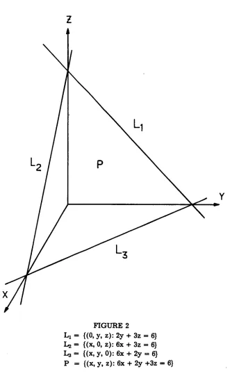
Here L1, L2, L3, and P denote three lines and one plane contained or
embedded in the three-dimensional space E3.
Although the physical intuition of most individuals declines sharply past three-dimensions, physicists have found many applica-tions of the idea of dimensional space consisting of all four-tuples (xI, x2, x3, x4) of real numbers. Such four-dimensional spaces
appear regularly in the theory of relativity.
Actually, many situations arise in which an n-tuple (x1, x2,
xn) of real numbers makes perfectly good sense. For example, sup-pose that one examines all the cases which have been decided in the Connecticut Supreme Court concerning zoning amendment ap-peals. A study of these cases may reveal a number of common is-sues. If a given issue, say change in the character of the
neighborhood denoted by x1, appears in the case, then x, takes the
value of 1 while if it does not appear x, takes the value 0. A partial list of issues and their labels x1, x2, etc. might consist of
x, change in the character of the neighborhood x2 the new use is not needed
x3 the new use is compatible from an economic standpoint
x4 the new zone change is detrimental to the neighborhood
x5 the character of the neighborhood supports the change (along with perhaps a hundred and forty-five others).
A lawyer might use five-tuplets to describe such patterns, i.e., the five-tuplet (0, 0, 1, 1, 1) could denote the situation where, x, = 0, denotes there has been no change in the character of the neighbor-hood, x2 = 0, the new use is needed, x3 = 1, the new use is
compati-ble from an economic perspective; x4 = 1, the zone change is
detrimental to the neighborhood; x5 = 1, the character of the
neigh-borhood supports the new use. If there are 150 issues, then a 150-tuplet of the general form
(X1, X2, . . , X X14 9, X15 0)
describes a general fact pattern. Mathematicians call a space made
up of n-tuplets (xI, x2, . . . , Xn) an n-dimensional space. Lines,
planes, and three-space are examples of geometric objects which mathematicians call manifolds. A line L constitutes a linear
sub-manifold of a plane P which contains it, while P itself may be a
lin-ear submanifold of a three-dimensional manifold E3 (ordinary Euclidean space). The list of manifolds includes the n-dimensional spaces mentioned above which are referred to as n-dimensional
manifolds.
of the algebraic equations used to describe the subspace. Equations of the form
ax + by + c = 0, and ax + by + cz + d= 0
are called linear equations; the first is linear in the two unknowns x and y, and the second in the three unknowns x, y and z. An expres-sion of the form
alxl + a2x2 +. . + anXn + c 0
is a linear equation in n unknowns X1, x2, • • . , xn. A line L is said to be linear, because the coordinates (x, y) of a point of L satisfy a linear equation in two unknowns, while a plane P is said to be linear because the coordinates of a point (x, y, z) of P satisfy a linear equa-tion in three unknowns. The set
Hn = ((x, x2, • • • , xn): ajx1 + a2x2 + •. + a.xn = c}
is called an affine hyperplane of the space En. A hyperplane is a lin-ear submanifold of En since the coordinates of any point Hn satisfy a linear equation in n unknowns, x1, x2, • - - , x.
The number of data points required to determine a line L = {(x,
y): ax + by + c = 0) is two, as can be seen with a piece of paper and a
straight edge. Frequently people wish to represent a set of data con-taining more than two points by the most suitable or best straight
1980] MATHEMATICAL MODELS FOR LEGAL PREDICTION 835
FIGURE 3
There are many mathematical techniques for determining such a line with the "method of least squares" being one of the most popu-lar, while drawing the line by eye is generally satisfactory for a small number of points.
All the manifolds mentioned above are of infinite extent, but
~Y
FIGURE 4
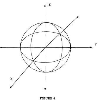
The algebraic equation satisfied by the coordinates (x, y, z) of each point of a sphere S of radius 2 is x2 + y2 + z2 = 4. Except for small perturbations due to mountains, valleys, and volcanoes, the earth is almost a sphere, although men for generations thought it was a plane. This property of looking like a plane locally is the fun-damental characteristic of a two-dimensional manifold.
19801MATHEMATICAL MODELS FOR LEGAL PREDICTION 837
x
FIGURE 5
FIGURE 6
19801 MATHEMATICAL MODELS FOR LEGAL PREDICTION 839
C
20
10L
5-n
FIGURE 7
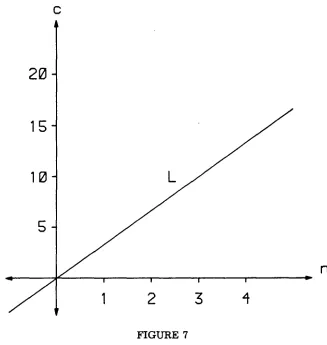
with the property that when the number of letters n increases by 1 unit, then the cost c increases by 5 units. Disregarding the fact that the symbol n is physically meaningful only when it denotes an inte-ger or whole number, it is a geometric fact that c increases by 5 units on the graph when n increases by 1 unit no matter where one starts, whether at an integer or not. Mathematicians say that the
rate of change of c with respect to n is 5 and denote this rate by the
symbol dc/dn. If the monthly overhead of running a law office de-pends on five independent factors denoted by x1, x2, x3, x4, and x5 with the respective unit costs (or rates of change) Pi, P2, P3, P4 and
P5, then the total overhead cost is given by
C - pIXl + p2x2 + p3x3 + p4x4 + p5x5.
change remains the same, namely, it is the increase in c with re-spect to a unit increase in any one of the five quantities X1, x2, x3, x4
and x5 and the notation is still much the same, i.e., the five rates of
change are denoted, respectively, by the symbols dc/dxl = Pl,
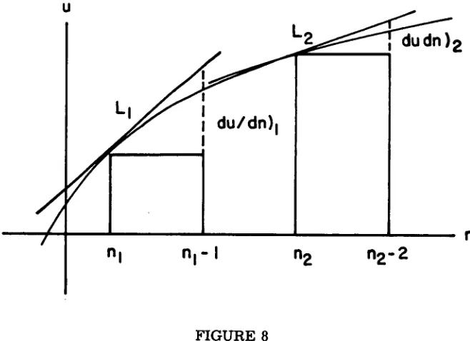
dc/dx2 = P2, dc/dx3 = P3, dc/dx4 = P4, and dc/dx5 = P5. These rates of change are all constant because the previous functional descrip-tions are all in terms of linear models useful in many cases but somewhat deficient in others. To illustrate the distinction between linear and nonlinear models, consider a variable u depending upon a variable n through a function relation with the graph sketched in Figure 8.
U
n
n
In
I- I
n
2n
2-2
FIGURE 8
When the functional relationship between u and n is nonlinear as above, then it becomes necessary to speak of the instantaneous rate
of change du/dn)1 of the variable u with respect to the variable n
when, for example, n = nj.
Mathematicians invented a method for computing this instanta-neous rate of change some two hundred years ago, but a rather good estimate can be had by merely drawing the line L1 of Figure 8 which
1980] MATHEMATICAL MODELS FOR LEGAL PREDICTION 841
L1). The slope m, is equal, by definition, to the instantaneous rate
of change of u with respect to n at the point (nj, ul), and also equal to the length of the dotted vertical line at nj + 1. A similar "best
straight line or linear approximation" to the curve at (n2, u2) is
given by the line L2 whose equation is u = m2n + b2 so that the
in-stantaneous rate of change du/dn)2 equals M2, numerically the
same as the length of the dotted vertical line at n2 + 1. The
instanta-neous rate of change of u with respect to n is clearly larger at (nj,
ul) that it is at (n2, u2).
I. LINEAR MODELS
The method of linear models relates to the concept of "best linear fit" as illustrated in Figures 3 and 8, but in most situations re-searchers generally apply the method to n-dimensional hyperplanes in (n + 1)-dimensional space. There the x-axis of Figure 3 becomes an n-dimensional "coordinate hyperplane" and the vertical y-axis re-mains as shown. The data to be fit consists of a collection of P1, P2,
• . .of "points" of the form (y, x1, x2, . . . , x,) requiring an addi-tional subscript to distinguish one point from another as indicated below:
P1 = (Y1, x11, x12, ,Xn)
P2 = (Y2, x2 1, x2 2, ... ,x2) P3 = (Y3, x31, X3 2, . . • , X3 n)
One can imagine P1, P2,. .. ,Pk points scattered about an (n +
1)-dimensional data space En+1 so that the problem is one of
determin-ing the best linear approximation, as in the case of the line in Fig-ure 3.
As previously mentioned, mathematicians have developed vari-ous techniques for finding such a "best hyperplane", but the most popular method is probably that of least squares. This method selects the desired hyperplane so as to minimize the sum of the squares of the distances from the hyperplane to the data points. Many computer programs are available to perform these kinds of calculations. All lead to a linear expression for y in terms of the
variables x1, x2,. .-. ,xn of the form
y = alx1 + a2x2 + . .- + anXn + an+l
where the a's have been determined so as to minimize the sum of the squares. Generally, statisticians prefer to have many more data points P1, P2, . . , Pk than variables x1, x2,- ... ,xn since this allows
them to make informed estimates about the accuracy of the deter-mination of the a's, but the present article does not explore this point.
The use of linear predictors of the outcome of court decisions has been advocated for at least twenty years. Some of the first inno-vaters were Fisher,7 Schubert,8 and Baade.9 Perhaps the most ac-tive person in the field has been Reed Lawlor.10 The person who has achieved the widest acclaim is undoubtedly Haar who, with Sawyer and Cummings, made a year long study of zoning amendment cases brought before the Supreme Court of Connecticut. The model of Haar is described in detail in the American Bar Foundation
Re-search Journal" and has recently enjoyed great success. According
to the Commercial Law Journal, the model of Haar gave the correct predictions in ninety-nine percent of over one thousand cases se-lected from a variety of states.12 Even without this surprising rec-ord, it is well worth considering the work of Haar and his associates as a tutorial in methodology.
Haar, Sawyer and Cumming formed a team of two lawyers and one statistician to make a statistical study with the aid of a com-puter of the zoning amendment cases decided by the Connecticut Supreme Court. The two lawyers identified a collection of 167 issues from seventy-nine cases heard by the Connecticut court over a pe-riod of roughly twenty years. Only forty of the issues proved signifi-cant when statistical tests were run.13 Since seventy-nine cases supply too little data for a good linear fit in a 41-dimensional space, the investigators used a method of analysis which groups the vari-ables having similar effects on the outcome into subsets, called
scales.14 As a result of this procedure, called factor analysis, the variables were grouped to form the eleven scales listed below:
Scale 1 Compatibility Indicated by Change in the Charac-ter of the Neighborhood
Scale 2 Use not needed
Scale 3 Adequate Physical Planning
Scale 4 Public Interest Planning and Zoning Techniques Scale 5 Compatibility from an Economic Perspective Scale 6 Zone Change Detrimental
7. See Fisher, The Mathematical Analysis of Supreme Court Decisions: The Use and Abuse of Quantitative Methods, 52 AM. POL. Sci. REV. 321 (1958).
8. See JuDiciAL DECISION-MAKING (G. Schubert ed. 1963).
9. See JURIMETRICS (M. Baade ed. 1963).
10. See Lawlor, Foundations of Logical Legal Decisions Making, M.U.L.L. 98 (1963).
11. Haar, Sawyer, & Cummings, Computer Power and Legal Reasoning: A Case
Study of Judicial Decision Prediction in Zoning Amendment Cases, 1977 AM. B.
FouND. RES. J. 651 (1977) [hereinafter cited as Haar]. 12. 85 CoM. L.J. 270 (1980).
13. Haar, supra note 11, at 711.
1980] MATHEMATICAL MODELS FOR LEGAL PREDICTION 843
Scale 7 Physical Services Inadequate
Scale 8 Compatibility Indicated by Large Uniform Blocks Scale 9 Good Planning Practices
Scale 10 Character of Area Supports Change Scale 11 Large-Area Zoning'5
The investigators retained two of the original variables in the re-gression analysis (statistical language for linear fits and linear pre-diction models):
011 The Court of Common Pleas Approved/Denied the Zone Change
012 The Zoning Authority Denied/Approved the Zone Change
They omitted these two variables from the factor analysis, since they had previously decided to include them in their linear predic-tor.16 The research of Haar and his colleagues produced three
mod-els of the general form
P=A+CV,+. .-+CkVk
where A = 0.56523 and the values of the coefficients C, ... , Ck are
listed in Table 1 below.17
TABLE 1
COEFFICIENTS OF THE LINEAR MODELS
Model with Model without Variable Basic Model Scale 9 added Scale 4
Scale 4 .05769 .05518
-Scale 6 -. 19320 -. 18397 -. 19139
Scale 7 -. 25548 -. 24747 -. 25450
Scale 8 .21506 .20939 .21336
Scale 9 - .04473
-Scale 10 .05265 .05629 .06746
Scale 11 .11884 .10477 .12014
Var. 011 .16121 .16510 .18324
Var. 012 -. 55106 -. 53905 -. 59198
The linear predictor for the Basic Model can be written P =
0.56523 + 0.05769S4 - 0.1932 S6 - 0.25548 S7 + 0.21506 S8 + 0.05265 S,0
+ 0.11884 5,, + 0.165 Vol,- 0.55106 V012. The variables S6, . . . , V012 assume only the values 0 and 1 so that those terms with plus signs designate issues primarily for plaintiff and those with minus signs those issues primarily for defendant.
Based upon the facts of a particular case, e.g., the Court of Com-mon Pleas has approved, so that Vol, = 1 or has disapproved, so that Vol, = 0; the Zoning Authority denied the zone change, so that Vol,
= 1 or will have granted the change so that Vol, = 0, and so forth for the remaining variables, one obtains a numerical value for P. Under the conventional notion that plaintiff wins with a preponderance of the evidence in his favor, the linear model predicts victory for plain-tiff whenever the entries for the given fact pattern produce values greater than 0.5 for P.
Haar and his associates reported the interaction of their linear predictor with predictions by conventional legal analysis.18 Haar as-serts that this sort of approach leads to a better organized attack on a legal problem, since preparation for computer analysis requires a very systematic examination of the cases.19 Furthermore, he claims that computer modelling displays the ratio decidendi20 of the case as a relationship between the facts and outcome, which can be mathematically expressed to the extent that the lawyer can ascer-tain precisely what facts were before the court.21 Moreover, the close reading required for computer analysis of the case improves the determination of the key factors in a case-by-case evaluation.2 2 Finally, this type of organization eases the task of a newcomer in the selected area of law by the systematization of the material.23
II. CATASTROPHIC MODELS
Researchers have developed two basic approaches to the theory of catastrophes which may be called, in the spirit of physics, the
the-oretical approach and the phenomenological one. Rene Thom
cre-ated the theoretical while Christopher Zeeman crecre-ated the
phenomenological. The next several pages discuss Thom's method
on which the models of Zeeman are based. Readers wishing to skip the theoretical discussion may proceed to subsection II.B infra which introduces the ideas of Zeeman.
A. Thorns Theoretical Approach
Thom invented his theory by means of ideas apparently bor-rowed from classical mechanics, since the rate of change of a key va-riable depends on a potential, of which the most familiar are those created by gravity. A skier standing at the crest of a ridge must ex-ercise great care merely to maintain himself there while, to the con-trary, one located in a valley must exert great effort to get out. The
19801 MATHEMATICAL MODELS FOR LEGAL PREDICTION 845
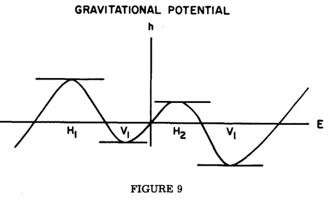
first skier is said to be in a position of unstable equilibrium and the second in a position of stable equilibrium. To fix the ideas, consider a cross-section of the country side assuming the form shown in Fig-ure 9.
GRAVITATIONAL POTENTIAL
h
FIGURE 9
GRAVITATIONAL POTENTIAL
Here the vertical variable h represents height above sea level while the horizontal variable E represents a line in an East-West direc-tion. The position determined by H1 denotes the crest of a hill on
which a particle, say a marble, would remain balanced if it were not displaced "at all" from its position. Physicists and catastrophe theo-rists refer to such a point as one of unstable equilibrium. The posi-tion V1 depicts the bottom of a valley at which the marble would
return even f displaced a small distance. Theorists call this a point of stable equilibrium. H2 and V2 locate additional unstable and
FIGURE 10
This figure illustrates three kinds of critical points which are naturally related to the stable and unstable equilibrium points of Figure 9. The reader should not allow the picture to suggest these exhaust all possible kinds of critical points since they form but a small selection. The points H, V, and P represent critical points which could be called hills, valleys, and passes. Only the valleys are stable equilibrium points; the other two are unstable.
These figures illustrating gravitational potentials display certain aspects of catastrophe theory whose potentials depend on auxiliary variables called control parameters. One of the simplest potentials occurring in the theory is
V(a, x) = x3/3 - ax
1980]MATHEMATICAL MODELS FOR LEGAL PREDICTION 847
V V V
0<0 o-0 o>0
FIGURE 11
CATASTROPHIC POTENTIALS
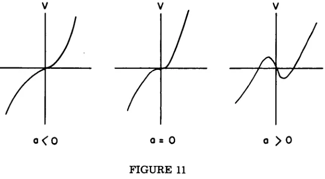
Geometrically, these graphs show no equilibrium point when a is negative, one unstable equilibrium point at the origin when a equals
0, and two equilibrium point at the origin when a is positive, namely,
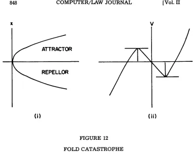
an unstable equilibrium point at x = -a and a stable equilibrium point when x = a. These equilibrium points may be determined from the rate of change dV/dx, which has the form (the negative is used in catastrophe theory)
-dV/dx = -x 2 + a = -(x 2 -a).
They are those points determined by values of x for which the rate of change dV/dx is zero, i.e., that satisfy the equation
x2- a = 0
x
V
ATTRACTOR
REPELLOR
i)
(ii)FIGURE 12
FOLD CATASTROPHE
The relation x2 - a = 0 generates two functions, x = a and x =
-a. The graph of the first gives the upper branch labeled attractor and that of the second gives the lower branch labeled repellor in Figure 12(i). If a = 1, the potential V(l, x) has an unstable equilib-rium point at x = 1 as shown in Figure 12(ii). This choice, a = 1, il-lustrates the fact that x-values on the upper (attractor) branch of Figure 12(i) correspond to stable equilibrium points while x-values on the lower (repellor) branch correspond to unstable equilibrium points.
1980] MATHEMATICAL MODELS FOR LEGAL PREDICTION 849
The original investigators based their analysis on equations of the form
(1) dx/dt = -dV/dx
which relate the rate of change of the response x with respect to t to the rate of change of the potential V with respect to x. They called the resulting process a gradient system. The potential V(a, x) =
X3/31 - ax, depending on a single control parameter a, generates the simplest gradient system having a behavior manifold like that of Figure 12(i) with a single catastrophe point. The next simplest type of catastrophe has a potential with two control parameters, a and b, with the expression
(2) V(a, b, x) = x4/4 - ax - bx2/2. This potential gives rise to the gradient system
(3) dx/dt = -(x 3 - a - bx).
For this system, the behavior manifold is the set of points in E3 sat-isfying the relation
(4) x3 - a - bx = 0.
This relation graphs into a two-dimensional submanifold of the three-dimensional manifold E3 of all points of the form (a, b, x). The control space of this process is the a,b-plane consisting of all points with coordinates (a, b, 0). Figure 13 presents these details pictorially.
In our initial example, the catastrophe set consisted of a single point, but in the present it is the subset of the behavior manifold de-fined by
(5) C = ((a, b, x): 3X2 - 0}.
This catastrophe set C is a one-dimensional curve contained in the two-dimensional behavior manifold. It forms the boundary of the cross-hatched area of Figure 13 and projects downwards into a curve B called the bifurcation set located in the control space. The behav-ior manifold is "pleated" into a sort of tuck over the region R bounded by the bifurcation set, i.e., there are three distinct surfaces over the region R. The curve C separates the cross-hatched surface from an upper surface called judgment for plaintiff and a lower sur-face called judgment for defendant. This Judicial Model takes the vertical or x-axis as a judicial axis representing the outcome of a given fact pattern. Such a fact pattern is described by means of two auxiliary axes D and P, D denoting the evidence and argument for the defense and P denoting the evidence and argument for the plaintiff. The variables D and P are related to the control parame-ters a and b by two linear equations, such as
a = c11D + c12P + c13
We will spare the reader any further mathematical analysis and finish with a few remarks. It may be worthwhile to attempt to sum-marize in a single paragraph some of the astounding achievements of Thom. He showed that the exceptional or singular points of gra-dient systems, determined by equations such as Equation (1) above, could be classified into a finite number of "relatively simple" types, just as a lawyer might classify legal issues as procedural or substan-tive. These types give rise to a family of standard models, whose features depend, among other things, upon the number of control parameters in a standard potential. Not surprisingly, the complexity of the standard model increases as the number of control parame-ters in the standard potential increase. The present survey has been limited to the cases of one or two control parameters which lead, respectively, to the fold catastrophe of Figure 12 and the cusp
catastrophe of Figure 13.
B. Zeeman's Phenomenological Approach
1980] MATHEMATICAL MODELS FOR LEGAL PREDICTION 851
THE CUSP CATASTROPHE
JUDGMENT FOR PLAINTIFF
CONTROL' SPACE
SET B
FIGURE 13
a serious problem involving the development of the required non-linear statistics. Cobb has made a promising beginning by returning to basics and incorporating a stochastic noise term into the standard potentials.24
Prior to the development of a rigorous statistics, there had been a flourishing evolution of ad hoc models in various social sciences
24. Cobb, Stochastic Catastrophe Models and Multimodal Distributions, 23
inspired by the pioneering work of Christopher Zeeman.25 In the spirit of the physics motivating much of the earlier work, we refer to his methods as the Zeemanian Process. The following discussion depends substantially on insights cultivated by reading Zeeman's treatment of institutional disturbances.26
The fact pattern underlying a judicial decision comprises issues that may be classified either as (1) evidence and argument support-ing the position of plaintiff denoted by the symbol P, or (2) evidence and argument supporting that of defendant denoted by D. In law, of course, who is plaintiff and who is defendant may depend on which party wins the race to the court house, rather than on the nature of
the dispute involved.
In civil cases, plaintiff wins his case if the trier of fact, some-times a judge and somesome-times a jury, finds a preponderance of the evidence in his favor. Considering D and P as conflicting factors in a judicial process enjoying a suitably discontinuous behavor, one ar-rives by means of the Zeemanian process at:
Hypothesis I. The standard model of the judicial process is a
cusp catastrophe with plaintiffs evidence and argument denoted by P and defendant's evidence and argument denoted by D as conflict-ing factors determinconflict-ing the outcome.
Figure 13 represents the standard model of the cusp catastrophe with the behavior manifold divided into parts-an upper part de-noted as judgment for the plaintiff and a lower part dede-noted as
judg-ment for defendant. Observe that in a V-shaped region loosely
centered between the P and D axes these two pieces overlap with the upper surface joined to the lower by a cross-hatched area bounded by the catastrophe curve. The catastrophe curve projects downward into the bifurcation set which lies in the control space. Using nomenclature introduced in the theoretical discussion, both judgment for plaintiff and judgment for defendant are attractor sur-faces which implies by the general theory that they are sursur-faces of stable equilibrium while the cross-hatched surface joining the two is a repellor, a surface of unstable equilibrium.
As intended, these terms indicate that, with certain exceptions to be discussed below, the state of the case is (defined by a point on the behavior manifold that indicates a victory either for plaintiff or for defendant at any given time). If the state of the case is repre-sented by a point on judgment for plaintiff, then it tends to remain there, while if it is represented by a point on judgment for the
de-25. Probably one of the most useful sources of information on his techniques is
E. ZEEMAN, note 5 supra.
1980] MATHEMATICAL MODELS FOR LEGAL PREDICTION 853
fendant then by stable equilibrium it tends to remain there. A state of the case in which the outcome is uncertain corresponds to a point on the cross-hatched surface representing a situation of unstable equilibrium. Thus, continued introduction of evidence and further argument soon displaces the state either to judgment for plaintiff or judgment for defendant.
Since plaintiff normally addresses the court first, unless the case is dismissed for failure to state a cause of action, his attorney should be able to secure a position (D, P) in the control space, say K, determining a state belonging to judgment for the plaintiff. Start-ing with the situation at K, the defense attorney must try to drive the point on judgment for plaintiff onto the surface judgment for de-fendant. One method might be by producing evidence of perjury or of a damaging admission by plaintiff to reduce the value of P (evi-dence and argument for plaintiff) and move the state along the dotted path on the behavior manifold from U (above K) to V (above H). A second method might be to produce overwhelming evidence and argument for defendant so as to move from the point K of the control space to the point H along the dotted path in Figure 14, thereby reaching the same state V in judgment for defendant. This last path illustrates two phenomena of catastrophe theory.
The first is the concept of delay caused by overlapping of judg-ment for the plaintiff and judgjudg-ment for defendant above the region R bounded by the bifurcation set. As one moves along the indicated path from K to H, the state of the case remains on the upper surface of judgment for plaintiff all the way over to the point on the catastro-phe curve lying above J on the bifurcation set. As a result, the favorable state desired is delayed beyond the point where it nor-mally should have occurred. The second is the phenomenon of
cata-strophic jump. When the motion reaches a point on the catastrophe
CATASTROPHIC PATH FROM K TO H
D
p
FIGURE 14
Small shifts occur in the structure of judicial catastrophic sur-faces for a variety of reasons. For example, society contains many natural plaintiff-defendant pairs including mortgagees versus mort-gagors, creditors versus debtors, and insureds versus insurors, along with hundreds more who are eternally trying to better their posture before the courts. As a consequence, many of them lobby for favorable legislation, litigate propitious rather than unpropitious cases, and include one-sided clauses favoring themselves in their contracts.
Hypothesis II. There is a continuing tendency for the judicial
process to avoid the extremes of "judgment for the plaintiff" or "judgment for the defendant."
particu-1980] MATHEMATICAL MODELS FOR LEGAL PREDICTION 855
lar case off the table locus on occasion. As a consequence, there may rise catastrophic transfers from the mere presence of noise in
the system. Zeeman offers this observation as a hypothesis.
Hypothesis III. External events, or internal incidents within the
judicial system may be represented as stochastic noise.
As this completes the description of catastrophic models, the discussion now turns to the method of nearest neighbours.
III. NEAREST NEIGHBOUR RULE
In their book on numerical taxonomy, Sneath and Sokal define their subject to be "the grouping by numerical methods of taxo-nomic units into taxa on the basis of their characteristic states. '27 These two scientists applied their methods primarily to biological sciences in which elaborate classification schemes have developed since the invention of taxonomy by Linnaeus in the eighteenth cen-tury. After the advent of large scale computing machinery, re-searchers introduced numerical methods into the subject. During the last quarter of a century, their procedures have spread from bi-ology into many other areas, particularly medicine.
The emphasis on empirical analysis of data leads naturally to what may be called the "operational approach to taxonomy," by analogy with P. W. Bridgman's ideas.2 8 In such a context "opera-tionalism" implies that statements and hypotheses about a subject, law for instance, are subject to meaningful questions that can be tested by observation and experiment. In law, to determine whether Case A is more related to Case B than it is to Case C, clear defini-tions must be given of what is meant by "more related," that is, by what criteria "more or less relatedness" can be measured. This leads to the notion of assigning a set of characteristics to cases to divide them into groups or classes.
For example, Case A belongs to Tax Group 1 if, and only if, Case A has certain characteristics, i.e., belongs to that collection of cases concerned with (1) income tax, (2) gross income, (3) prizes, (4) treasure trove, (5) possession .... Thus, a case belongs to a partic-ular Tax Group if, and only if, it possesses all characters from a de-fining list. A group of cases so determined will be referred to as a
monothetic group.
Under this format, a group of cases is defined by reference to a set P of properties which are both necessary and sufficient for
bership in the class. It is possible, however, to define a group G in terms of a set
P=PI,. •.Pn
of properties in a somewhat less restrictive manner. Suppose we have a collection of cases such that
1) Each one has a large number of the properties in P. 2) Each p in P is possessed by large numbers of these
indi-viduals, and
3) No p in P is possessed by every individual in the aggre-gate.
According to condition 3, no single property p is necessary to membership in the collection; and nothing has been said to warrant or rule out the possibility that some p in P is sufficient for member-ship in the aggregate. A group of cases is polythetic if the first two conditions are fulfilled and is fully polythetic if condition 3 is also fulfilled. Wittgenstein has emphasized the importance of these ideas in ordinary language and especially in philosophy.2 9 The com-mon example in law of a line of cases tends to represent a fully
polythetic group or collection of cases.
We introduce the following cases as illustrations of the ideas we have discussed.30
CASE A: Cesarini v. United States31 concerned a tax defi-ciency declared by the Commissioner on the basis of some $4,500 found by the Cesarinis in a piano purchased in 1957. Having discov-ered the money in 1964, they reported it as ordinary income for that year. Later, the Cesarinis tried to amend their return, claiming there was either no tax due at all on the money was, at most, capital gains. The Circuit held the amount was ordinary income. Charac-ters: 4, 6, 17, 23, 31, 34, 42, 49, 54, 55, 56, 61, 70, 71, 73, 74.
CASE B: Old Colony Trust Co. v. Commissioner32 treats the claim of the government that W. M. Wood was in receipt of income whenever his company, American Woolen Company, paid his taxes of 1918 and 1919, that is, the payments made to the Internal Revenue Service by the company represented income to Mr. Wood. The Supreme Court agreed with the Commissioner. Characters: 10, 11, 13, 20, 28, 34, 48, 50, 63, 64, 68.
CASE C: Commissioner v. Glenshaw Glass Co. 33 raised the is-sue of whether money received as exemplary damages for fraud or
29. Id. at 21.
30. See Table 2 infra for a list of key characters for income tax cases.
31. 396 F. Supp. 3 (N.D. Ohio 1969), afd per curiam, 428 F.2d 812 (6th Cir. 1979). 32. 279 U.S. 716 (1929).
1980] MATHEMATICAL MODELS FOR LEGAL PREDICTION 857
for treble-damages in an antitrust recovery must be reported as
gross income. The Supreme Court held these to be taxable income. Characters: 2, 6, 16, 25, 27, 31, 33, 34, 40, 56, 57, 68.
CASE D: Chandler v. Commissioner3 4 considered whether or not the furnishing of a house to a principal stockholder by a corpora-tion resulted in income to the stockholder. Characters: 24, 34, 59, 66, 68.
CASE E: J. Simpson Dean35 contemplated whether Dean and
his wife were required to pay certain income tax in view of an inter-est-free loan granted to them by the Nemours Corporation. The
Supreme Court held no. Characters: 3, 7, 9, 13, 18, 28, 34, 61, 66.
CASE F: Commissioner v. Duberstein3 6 concerned the case in which Duberstein received a Cadillac as a gift from Berman. Berman stated that the Cadillac was a gift in return for business fa-vors of Duberstein, but deducted the cost as a business expense. The Court held that the car represented income to Duberstein. Characters: 4, 5, 8, 12, 15, 18, 28, 30, 31, 34, 55, 58, 60, 62, 63, 64.
These cases will be used to illustrate the basic concepts of
monothetic and polythetic classes of cases.
The small selection of characters which follows illustrates the concept of polythetic.
CHARACTERS CASES
A B C E F
6 Capital 1 0 1 0 0
13 Consideration 0 1 0 1 0
28 Gift 0 1 0 1 1
31 Gross 1 0 1 0 1
In this example, the defining set P of characters consists of the set 6, 13, 28, and 31. Each of the cases from the set A, B, C, E, F heads a column which determines whether or not a given character occurs in the header case. Thus, Case A contains the character 6 [Capital] denoted by the presence of the 1 in the first row of column A while it does not contain the character 13 [Consideration] indi-cated by 0 in the second row of column A. Case B contains the char-acter 13 [Consideration] as indicated by the appropriate 1 in row 13 of column B, but does not contain 6 [Capital] as indicated by the 0 in row 6 of column B.
Note that the table reveals the. following three properties.
34. 119 F.2d 623 (3d Cir. 1941).
i) each column, that is, each case contains fifty percent (a substantial percentage) of the characters,
ii) each character is contained in a large number of cases, and
iii) no character in P is contained in all the cases.
This is an example of a class of cases which is both polythetic and
fully polythetic.
A second table has been constructed to illustrate the concept of
monothetic using the same collection of cases, but now restricting P
to only the two characters 34 [Income] and 68 [Tax].
CHARACTERS CASES
A B C D E F
34 Income 1 1 1 1 1 1
68 Tax 1 1 1 1 1 1
Each of the cases deals with the federal income tax. More precisely, these cases A through F form a small selection from the monothetic class of federal income tax cases, this last class containing a case if, and only if, it has the characters 34 and 68.
These examples are intended as an explanation, not only of what is meant by a monothetic or polythetic class of cases, but also as examples of what is meant by a legal taxonomic relationship. The concept of a legal taxonomic relationship can be greatly refined by attaching a certain legal meaning to various standard words from biological taxonomy such as: phyletic, phenetic, cladistic, and a ge-neric. However, this description should be adequate to indicate the general direction of taxonomic research.
TABLE 2
KEY CHARACTERS FOR INCOME TAX CASES
1 Account 38 Internal
2 Antitrust 39 Joint
3 Assignment 40 Legal
4 Awards 41 Legislative
5 Benefit 42 Limitation
6 Capital 43 Loan
7 Case 44 Moral
8 Code 45 Motive
9 Company 46 Nondeduction
10 Compensation 47 Note
11 Commission 48 Obligation
12 Compensated 49 Ordinary
13 Consideration 50 Payment
1980]MATHEMATICAL MODELS FOR LEGAL PREDICTION 859
15 Customer 52 Period
16 Damages 53 Personal
17 Deduction 54 Possession
18 Deficiency 55 Prizes
19 Donative 56 Profits
20 Employer 57 Receipts
21 Exemplary 58 Refund
22 Exclusion 59 Rental
23 Exempt 60 Resign
24 Expenditure 61 Return
25 Fraud 62 Retirement
26 Free 63 Revenue
27 Gain 64 Salary
28 Gift 65 Shares
29 Grace 66 Stock
30 Gratuity 67 Stockholder
31 Gross 68 Tax
32 Holding 69 Taxable
33 Illegal 70 Treasure
34 Income 71 Trove
35 Indebtedness 72 Trust
36 Intent 73 Waiver
37 Interest 74 Windfall
The general philosophy of numerical taxonomy generates a number of classifying techniques, many of which are well described in the very useful book by John Hartigan of Yale on clustering algo-rithms.37 Among other devices, Hartigan lists proffles, distances, quick partition algorithms, k-means algorithms, partition by exact optimization, drawing trees, and single-linkage trees. Each of these have applications to the classification and organization of complex data such as case law. Researchers have developed complicated computer packages, for example at SUNY Stony Brook, for carrying out computations on data introduced in a standard format.
In spite of a high level of activity in the general area, Mackaay and Robillard appear to have made perhaps the only application to the law.38 Their method depends upon the introduction of a distance
function to compare and distinguish cases on the basis of a
well-de-termined set of properties. They use the term descriptor in much the sense that this paper and most lawyers tend to use the term
is-sue. Nevertheless, the reader is warned that these authors use the
word in a more or less technical sense which itself has constituted a
37. J. HARTIGAN, CLUSTERING ALGORmTHMS 1975.
topic of research for some investigators.3 9
Mackaay and Robillard provide a convenient outline of a "gen-eral method" of predicting judicial decisions which can be presented as follows: (1) select a line of cases dealing with the problem at hand, (2) determine a set of descriptors (issues) by means of which the fact patterns of each case can be delineated, (3) make a careful legal analysis of the cases to fix the fact pattern of each with respect to these descriptors, (4) use any ingenious scheme which comes to mind to enhance these results, and (5) apply your prediction proce-dure to the results of (4).
They assert that the less homogenous the line of cases, the more general the issues and the less precise the prediction, and note that Lawlor has developed useful procedures for making key selections.40 Naturally, it is commonplace to examine the case in the usual lawyering fashion for such a determination of issues. For the purpose of linear analysis, the number of cases should be sub-stantially larger than the number of issues mentioned. Given other-wise, Mackaay and Robillard recommend factor analysis, remarking that Kort was one of the earliest to use it in legal analysis and not-ing that Lawlor suggested intuitive regroupnot-ing and scalnot-ing as an al-ternative.41
Before returning to the specifics of the distance function used by Mackaay and Robillard, perhaps it may be informative to note that a variety of distance functions have been used in numerical tax-onomy and cluster analysis, some of which have a statistical basis and some of which do not. Both Hartigan and Sokal discuss the choice of a distance function and related problems from a number of points of view.42
A case may be described by means of an n-dimensional, in this
case when using Table 2, a 74-dimensional vector (X1, x2, • • . , x74)
where x, = 1 if account is an issue and x, = 0 if it is not; x2 = 1, if anti-trust is an issue and x2 = 0 if it is not; . . ; x74 = 1 if windfall is
an issue and x74 = 0 if it is not. In these terms, two cases A and B are described by two vectors (xI, x2,. ... , x74) and (Y1, Y2, .. . Y74), respectively. Hamming defines the "distance" from Case A to Case B to be the number of places in which the two vectors differ and
de-39. See, e.g., R. Lawlor, Applied Jurimetrics-Case Law Analysis Manual (1969)
(unpublished paper); S. NAGEL, THE LEGAL PROCESS FROM A BEHAVIOURAL PERSPEC-TIVE, chs. 9 & 13 (1969).
40. Mackaay & Robillard, supra note 1, at 303-05, and elsewhere for a more nearly complete set of references to the important work of Lawlor in this area.
41. Id. at 303,305.
1980] MATHEMATICAL MODELS FOR LEGAL PREDICTION 861
notes the Hamming Distance by D(A, B).4 3 Investigators find a number of advantages and disadvantages in using this distance function, however, in many respects the particular form has little ef-fect on the clustering procedures developed around it, i.e., one can use different distance functions with the same clustering algorithms. Mackaay and Robillard developed a natural prediction proce-dure based on a line A1,. . ., A.4 of sixty-four cases concerned with
capital gains taxes in Canada.44 By means of legal analysis of these cases, they selected a collection of forty-six key issues so that each case Ai of the 64 determines a description vector VAi of a 46-dimen-sional description space E46. Any new case A provides a new description vector VA for which their program determines the
near-est neighbour, that is, that vector VAi which is nearest to VAi with respect to the Hamming distance. The predicted outcome for A is the actual outcome for Ai.
Of course, any scheme such as this reveals certain limitations in practice and serves as a basis for a better one. Consequently, the two researchers incorporated various improvements in their method which are reported in their paper.45 Probably the most impressive result of their investigation is a comparison of the predictions of a linear model of Lawlor, those of the method of nearest neighbours, and those of an experienced tax attorney. The results are very favorable and those decisions on which the prediction went wrong can frequently be classified as unusual.46
IV. CONCLUSION
This article has suggested the possibility of developing practical methods for the prediction of judicial decisions by mathematical methods. Two of the methods discussed, the method of linear mod-els of Haar, Sawyer and Cummings and the method of nearest neighbours of Mackaay and Robillard have shown themselves useful in practical applications. In particular, the method of Haar and his collaborators has correctly predicted ninety-nine percent of the deci-sions in over a thousand cases, so that in the area of prediction of Zoning Amendment cases there is remarkably little hope for im-provement. Such success provides both a real opportunity and a se-rious need for developing linear models in other special areas, not only to verify empirically that the method works in general, but also to provide additional predicting models for the legal profession.
43. Mackaay & Robillard, supra note 1, at 307.
While not reaching the level of precision of Haar, the method of nearest neighbours of Mackaay and Robillard has proved excellent as a predictor of capital gains cases in Canada. Continued research in the area of nearest neighbours can follow well-defined paths al-ready pursued to great depths by investigators in the biological and
medical sciences.