Outlier Mining Based on Neighbor-Density-Deviation with Minimum Hyper-Sphere

(1)

Outlier Mining Based on Neighbor-Density-Deviation

with Minimum Hyper-Sphere

Yiwei Yuan, Hui Cao, Yanbin Zhang, Qian Xie, Rui Yao

State Key Laboratory of Electrical Insulation and Power Equipment,

Electrical Engineering School, Xi’an Jiaotong University, Xi’an, Shaanxi, 710049, China e-mail: [email protected], [email protected], [email protected],

[email protected], [email protected]

http://dx.doi.org/10.5755/j01.itc.45.3.13164

Abstract. Outlier mining is to find exceptional behaviors of objects that deviate from the rest of the dataset or do not satisfy the common patterns. This paper introduces a density definition using the minimum hyper sphere and proposes an outlier mining algorithm based on neighbor-density-deviation. First, the definition of local space-density of an object is proposed by using the minimum hyper sphere. Second, the nearest neighbor sequence (NNS) based on the distance between an object and the neighbors of the object is established. After getting the space-density and the NNS of the object, the neighborhood density deviation (NDD) in NNS can be calculated based on the sum of density difference between the object and its neighbors. Finally, the neighbor-density-deviation-based outlier factor (NDDOF) is obtained to indicate the degree of the object being an outlier. To evaluate the effectiveness and the performance of the novel definition of space density and the NDDOF algorithm, we experiment on a synthetic dataset and three real UCI datasets. The results verify that the space-density is meaningful and the NDDOF algorithm has higher quality in outlier mining.

Keywords: Outlier mining; minimum hyper sphere; local-density; NDD; NDDOF.

1. Introduction

Outlier detecting is an important procedure in data processing. Hawkins describes an outlier intuitively as :“An outlier is an object that deviates so much from other objects as to be suspected that it was generated by a different mechanism”[1]. Outlier mining refers to the problem of finding characters in data that are very different from the rest of the data. Outlier mining could be used in lots of practical areas, such as for cleaning the clusters for machine learning method[2] , finding the abnormal usage of risk detection in finance [3], diagnosing illnesses from health care databases [4], strengthening the ability of extreme learning machine [5], improving the adaptability and the robustness in image matching [6], and identifying the network anomaly in supervisory system [7], etc.

In the researches of detecting outliers, most methods are developed based on statistics[8, 9]. These statistical-based methods need the distribution of the dataset as the prior knowledge[10-12], and the outliers should have different characters with respect to the distribution. Following the outlier definition, many works consider that outliers do not belong to any cluster and the object in clusters shall not be an

outlier [13, 14]. The outlier mining is dependent on the quality of clustering algorithm used [15]. Knorr and Ng proposed the distance-based definition of outliers, which is simple and intuitive [16], and Knorr et al. discussed the usefulness of the definition detailedly [17]. The object is regarded as an outlier by the distance-based outlier mining methods according to the distance between the object and its nearest neighbors [18]. These methods differ in the distance functions of the nearest-neighbors. The outlier mining methods based on distance are used conveniently, but they are sensitive to parameters the users choose and could not work well in dataset with different density regions.

(2)

density-based methods have a disadvantage that how to choose the parameters to define the neighborhood of an object [26]. As the algorithms are density-based, so how to define the density of an object reasonably is also difficult.

This paper proposes a density definition of an object named space-density and proposes an outlier mining algorithm based on density, and the outlying degree of an object is indicated by the neighborhood- density-deviation-based outlier factor (NDDOF). First, the k-nearest neighbors series(NNS) is established, and the novel concept of space-density of an object is presented using the minimum hyper sphere algorithm. Second, the neighborhood density deviation (NDD) in NNS can be calculated based on the sum of density difference between the object and its k-nearest neighbors. Finally, the NDDOF value is obtained by using the NDD to indicate the outlying degree of the object. The rest of this paper is organized as follows. In Section 2, we discuss the related outlier mining algorithms based on density. In Section 3, the density concept and the outlier mining algorithm are explained in detail. After proposing the algorithm, we analyze the time complexity of the algorithm. In Section 4, experiments results are discussed. Section 5 concludes the paper.

2. RELATE WORK

In this section, we review some definitions of density and classical density-based outlier mining algorithms.

2.1. Density definitions

The common definitions of the density are shown as follows [15]:

Definition 2.1. Given a positive number d, the density of an object is equal to the number of objects whose distance from the object is less than d.

Definition 2.2. The density of an object equals to the reciprocal of the average distance between the object and its k neighbors, and the k is a positive integer.

To improve the density definition, the k-density is proposed [27].

Lemma 2.1. The distance of object p, denoted as k-distance(p), is defined as the distance d(p, o) between p and an object of D such that:

a)for at least k objects o'∈ D \ {p}, it holds that d(p, o') <= d(p, o), and b)(ii) for at most k − 1 objects o'∈ D \

{p}, it holds that d(p, o') < d(p, o).

where D is the dataset and p is fall into D.

Lemma 2.2. An object whose distance from p is not greater than the given k-distance is one of the k-distance neighbors of p.

Let Nk(p) represent the k-distance neighborhood of p and it is used for defining the k-median-distance of p.

Lemma 2.3. Given any positive integer k, the k-median-distance of p, kmdist(p)is equal to the average of the distances between p and the k-distance neighbors and is formulated as:

kmdist(p) =median{dist(p, o)|o ∈

Nk(p)}, where dist is the distance between two objects.

Definition 2.3. The k-density is the quotient of the number of the k-distance neighbors and the k -median-distance of p and is formulated as:

kden(p) = |Nk(p)|/kmdist(p), where |Nk(p)| is the size of Nk(p).

2.2. Density-based outlier mining algorithms

The LOF in [19] is firstly used to quantify the outlying degree of an object. The value of LOF is obtained based on the average of the ratio of the local reachability density of p and those of its k-nearest neighbors. A parameter named MinPts is needed to determine the minimum size of the neighborhood of the object. It is clear that the larger the local reachability density of p is, and the lower the local reachability densities of MinPts-nearest neighbors of p are, the lower the LOF value of p is. This algorithm has only one parameter k, which is equal to MinPts, and the parameter strongly affects the outlierness of an object. If the parameter k is set to be too low, LOF

does not detect outliers which are close to a dense cluster; on the contrary, the small clusters may be regarded as outliers. A modification of the LOF

algorithm is LOF’, LOF" and GridLOF [21]. LOF’

simplifies the formula of LOF which is understanding easily, LOF" distinguishes between the neighbors for computing the density and the neighbors for comparing the densities of the neighbors of an object. The GridLOF reduces normal objects by using the grid based method and then computes LOF score.

INFLuenced Outlierness (INFLO) is outlier mining method proposed in [24]. The paper takes the nearest neighbors and the reverse nearest neighbors into account to estimate the density distribution of the neighborhood. Tang et al. figured that the objects are “connected” to the neighbors and presented an outlier factor based on connectivity between objects, named

COF in [23]. The COF of an object is the ratio of the average chaining distance from the object and the average of chaining distances from k-distance neighbors to its own k-distance neighbors. The COF

(3)

neighborhood density is similar to that of an outlier. Cao (2010) proposed a density-similarity-neighbor-based outlier mining algorithm(DSNOF) for outlier mining [27]. DSNOF constructs similar density neighbor (SDS) of each object, and the earlier objects in SDS influence greater to the object.

As Cao et al. explained, the LOF algorithm, the

INFLO algorithm and the COF algorithm can not distinguish between the outliers and the normal objects in the special dataset. Moreover, the value of k directly influences the outlier mining results of the

LOF algorithm, the INFLO algorithm, and the COF

algorithm. For a given object p, the k-neighbors of p may not have p as one of their own k-neighbors. Although the DSNOF algorithm has some effect on outlier mining, its density definition only takes the k- neighbors of the object p into account and ignores the objects whose k-neighbors contain p. So the outlier mining algorithm could be improved on density definition and some other aspects.

In the next section, we present a new definition of the density of an object and propose a novel density-based outlier mining algorithm.

3. The algorithm

In this section, we introduce the definition of the space density. In addition, we propose the outlier mining algorithm based on the space density and analyze the time complexity of the algorithm.

3.1. Space-density of an object

Definition 3.1. The smallest enclosing hyper sphere. An n-sphere is the extension of an ordinary sphere surface to n-dimensional space. As n being a natural number, an n-sphere is defined as the set of objects in (n+1)-dimensional Euclidean space which are at a certain distance from a central object, where the certain distance is the radius R which may be any positive real number.

Particularly:

a 0-sphere is the pair of points at the ends of a (one-dimensional) line segment,

a 1-sphere is the circle(two-dimensional), a 2-sphere is the two-dimensional surface of a (three-dimensional) ball in three-dimensional space.

Spheres of dimension n > 2 are called hyper-spheres[28].

The smallest enclosing hyper-sphere is containing the neighborhood of p with the smallest radius R.

Definition 3.2. The NNkand RNNkof p. The NNkis the set of the k-nearest neighbors of p. The reverse nearest neighbors (RNNk) of p are essentially objects that have p as one of their k nearest neighbors [24].

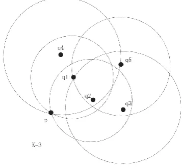
Figure 1 shows the constructing of RNNk. We assume that a dataset A = {p, q1, q2,q3, q4, q5}. For

k=3, the nearest neighborhoods of the points in A are

NNk(p) = {q1, q2, q3, q4}, NNk(q1) = {p, q2, q4},

NNk(q2) = {p, q1, q3}, NNk(q3) = {q1, q2, q5},

NNk(q4) = {p, q1, q2, q5} and NNk(q5) = {q1, q2, q3}, respectively. During the search of NNk of p, q1, q2,

q3, q4 and q5, RNNk(p) = {q1, q2, q4} is built. Similarly, RNNk(q1), RNNk(q2), RNNk(q3), RNNk(q4), and RNNk(q5) are found. It is obvious that the

RNNk(p) may not be equal to NNk(p).

Figure 1. Constructing of RNN

Definition 3.3. The effective neighbor points in the neighbors of p. For any positive integer k, the effective neighbor points exist in both the NNkand the RNNk of p, namely, ENP(p) = NNk(p)∩

RNNk(p). ENP(p) may be empty.

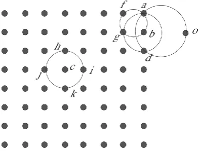
In Figure 2, D = {a, b, c, d, e, f, g, h, i, j, k}, when

k = 4, the k-neighbors of point d, NNk(d), is {e, g, h,

j}, and its RNNk(d) is {e, j}. NNk(g) = {e, f, h, i} and

RNNk(g) = {e, f, h, i, k}. The effective neighbor points

ENP(p) = {e, j} and ENP(g) = {e, f, h, i}, respectively.

Figure 2. The effective neighbor points

Definition 3.4. The space-density of an object p. Given any positive integer k, the space-density of p

(4)

In order to calculate the minimum hyper-sphere of the neighborhood, the number of points must be larger than the dimension of the points. In other words, the value of k should be greater than the dimension of the points.

It is obvious that the density of g should be larger than that of d in Figure 2. Following the definition, we can calculate the space-densities of d and g.

spden(d) =|ENP(d)|/R(d) = 2/R(d) and spden(g) =

|ENP(g)| /R(g) = 4/R(g). The radiuses of the two hyper-spheres are R(d) and R(g), respectively. As it is shown that R(d) > R(g), thus spden(d) < spden(g).

Figure 3. The space-density of each object for k=3

An example is shown in Figure 3. The point o is an outlier from a point set which is uniformly distributed. The distance between a and b is 1, and the distance between o and b is 2. The NNk(a) = {b, f, g}, NNk(b) = {a, d, g}, NNk(c) = {h, i, j, k}, NNk(o) =

{a, b, d} and RNNk(a) = {b, f}, RNNk(b) = {a, d, g},

RNNk(c) = {h, i, j, k} and RNNk(o) = ∅. R(a) = 0.707,

R(b) = 1, R(c) = 1 and R(o) = 1.25. We can calculate the densities, respectively. spden(a) = 2.828, spden(b) = 3, spden(c) = 4 and spden(o) = 0.

When the density definition is confirmed, we will introduce our outlier detecting algorithm based on the new density.

3.2. The NDDOF algorithm

In this subsection, the NDDOF algorithm is discussed detailedly.

Given a dataset D and a positive integer k, the

NDDOF algorithm is constructed as the following steps.

Step1. Calculate the distance between any two objects and find the k-distance neighbors of each object in D.

Step2. Construct the NNS of each object in D. Let p∈D and NNk(p) be the k-distance neighborhood of p. The nearest neighbor sequence of p is NNS(p), and NNS(p) = {p, c1, c2, … ,cr }, where r = |NNk(p)| and ci ∈

Nk(p), i = 1, 2,… ,r.

Construct the NNS is an iterative process. In each iteration, the nearest neighbor of p in the remaining objects of NNk(p), is picked up and added to the NNS(p) sequentially. If there are more objects have the same distance with p, they would be picked up in sequential order. Then the NNS(p) and

NNk(p) are updated. When all of the objects in NNk(p) are picked up, Step2 is finished and the NNS(p) is constructed. Using the same method, the NNS of each object in D

can be constructed.

Step3. According to Definition 3.4, compute the space-density of each object in D.

Step4. Define the space-density difference between two objects.

The space-density difference between x and

y, named △spden(x, y), is defined as:

△spden(x, y) = |spden(y) − spden(x)|,

so that △spden(x, y) = △spden(y, x).

Step5. According to the definition of △spden(x, y), calculate the neighborhood density deviation (NDD) of each object in D based on the

NNS. NDD(p) is viewed as the neighborhood density deviation of p in NNS, and the earlier objects in NNS contribute more in the NND. Let p be an object in D, and the neighborhood density deviation of p defined as:

1

( ) r_i ( , ) / ,i

NDD p 



_spden p c i

where r = NNk(p).

Step6. Compute the NDDOF value of each object in

D.

For any object p in D, the neighborhood-density-deviation-based outlier factor,

NDDOF(p), is expressed as:

( )

( ) ( ) ( ) / ( )

k

k o NN p

NDDOF p NN p NDD p



_ NDD o

The NDDOF value of p is the ratio of the NDD of

p and the average of the NDD of k-distance neighbors of the object. NDDOF indicates the degree of the object being an outlier, that is to say, the smaller the

NDDOF value is, the lower the outlierness of p is.

3.3. The time complexity of the algorithm

We assume that D consists of n objects and each object is n-dimensional, k is a positive integer, and

r (r ≥ k) is maximum number of the k-distance neighbors of the objects in D.

For the first step, the time complexity of computing the distances between any two objects is

(5)

Table 1. Outlier detecting results

rank index LOF index spLOF index INFLO index spINFLO index DSNOF index spDSNOF

1 o2 29.2 o1 50 o2 10 o1 10 o2 8.2 o1 50

2 o1 15.1 o2 50 o3 10 o2 10 o1 6.5 o2 50

3 o3 14.1 o3 50 o4 10 o3 10 o3 5.4 o3 50

4 o5 6.0 o4 50 1089 1.4 o4 10 o7 2.9 o4 50

5 o7 4.9 o7 49.3 1054 1.3 1291 3.5 o5 2.8 o7 3.0

6 o6 4.7 o6 22.6 1689 1.3 1379 3.3 o6 2.7 o5 2.3

7 o4 3.6 o5 19.7 1193 1.3 1080 2.7 438 2.3 o6 2.2

complexity is O(ndk2_{), The third step of the}

NDDOF algorithm is calculating the space-density of each object. Since computing smallest enclosing hyper sphere takes the most time of this step, the time complexity of Step3 is considered as the smallest enclosing hyper sphere complexity, which is less than

2 3/ 2

[ / ( / )(1/ ) lg(1/ )]

O nd  d  d  [29], where is

0.001. The forth step is calculating the space-density difference between any two objects, and the time complexity is O(n(n−1)/2). The fifth step and the sixth step are calculating NDD and NDDOF values of each object, respectively, and the complexities of them are both O(nk). Hence, the time complexity of the NDDOF algorithm is

2 2 2 3/ 2

[ / ( / )(1/ ) lg(1/ )].

O n dndk nd  d  d 

4. Experiments results

In this section, we will experiment on a synthetic dataset to test the effectiveness of the space-density and experiment on three real datasets to estimate the performance of the NDDOF algorithm. The synthetic dataset is similar to the dataset in [19]. The real datasets are real UCI datasets. To evaluate the effectiveness of the space-density, we will adopt our space-density definition to the LOF method, INFLO

method and the DSNOF method to form spLOF

method, spINFLO method, and spDSNOF method. After getting the new methods with space density, we compare the results between the LOF method with spLOF method, the INFLO method with spINFLO

method, the DSNOF method with spDSNOF method, respectively. To evaluate the performance of the

NDDOF algorithm, we compare the NDDOF

algorithm with the LOF algorithm, the INFLO

algorithm, the COF algorithm, and the DSNOF

algorithm. All the outlier detecting algorithms are implemented by MATLAB R2010a and the performance environment is a 2.9 GHZ Intel processor, with 8G of main memory, under Windows7 operating system.

4.1. Experiments on density

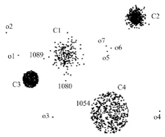
The dataset in Figure 4 shows a two-dimensional synthetic dataset.

The dataset consists of a small Gaussian cluster of 200 points named C1 with low density and three large clusters of 500 points each. Among these three clusters, C2 is a Gaussian distribution cluster with dense density and C3 and C4 are uniform clusters with different densities. There are 1700 normal objects in the dataset totally. Furthermore, it contains seven outliers which are o1, o2, o3, o4, o5, o6 and

o7.

Figure 4. Synthetic dataset

Table 1 lists the top-7 outliers established by each algorithm for k = 40. The rank lists the top 7 outliers each algorithm detects. The index represents the positions of objects. By visual comparison, the most outstanding outliers o1, o2, o3 and o4 can be recognized by each measure with new density definition while INFLO can not pick out o1 and

DSNOF can not find o4. Even more, although LOF

can find the top 7 outliers, the outliers found by the spLOF are more meaningful. Even for the same objects appearing in top-n lists of each measure, their positions could be different and new density-based results are obvious more reasonable. The points o1,

o2, o3 and o4 do not belong to any cluster, so the outlier factors of spLOF, spINFLO, and spDSNOF

are always the top 4 outliers while LOF, INFLO and

(6)

When k is increased, the results are similar. So the new density definition with minimum hyper sphere algorithm is of better effectiveness and more meaningful.

4.2. Precision, recall and rank power metrics

In this part, three important metrics, namely,

precision, recall and rankpower are introduced for estimating the performance of an outlier detecting algorithm[25, 27].

It is assumed that a dataset D = DO ∪Dn. DO is the set of all outliers and Dn is the rest of the dataset

D. For any integer m ≥ 1, Om denotes the set of outliers detected by an algorithm in the top m objects. The precision and recall with respect to m as follows:

| m| / , | m| / | o| .

precision  O m recall  O D

Precision is the ratio of outliers among the top m

ranked objects detected by the algorithm, while recall

is the ratio of the outliers included within the top m

ranked objects and the total outliers. Precision and

recall only evaluate the accuracy of the algorithm but can not reflect the true positions of the outliers. For example, three outliers located in the top three positions have the same values of precision and

recall with three outliers located in the bottom three positions among m objects returned while we are interested in the top ranked three outliers. To deal with the problem, rankpower is introduced to reflect the positions of the outliers among the results returned by an outlier algorithm [30]. Tang et al. revise the definition of rankpower. The rankpower

value ranges from 0 to 1. The larger rankpower value is, the better the performance of the algorithm can be [23]. Assume that the algorithm returns n outliers in

m objects, the rankpower is expressed as:

1 ( ) ( 1) / 2 ni i, RankPower m  n n 



_ L

where n ≤ m, 1 ≤ i < n and Li represents the position of the ith outlier.

It is clear that the larger precision, recall and

rankpower are, the more accurate and effective the outlier detection algorithm is.

4.3. Results on real datasets

To achieve a comprehensive understanding on the effectiveness of the NDDOF measure, we test the effectiveness of NDDOF algorithm on some real datasets with different sizes and dimensions to discover rare classes as pointed out by Yu and Aggrawal [31]. The method has been used in [15, 26, 32, 33]. Three real datasets, Pima Indians diabetes dataset, image segmentation dataset, and Johns Hopkins university ionosphere dataset, respectively, are adopted in the experiments. Because the number of the data that the minimum enclosing hyper-sphere algorithm needs should be more than that of the data

dimension, so k must be larger than d. In addition, we also test the influence of different k values on the three datasets. Nrc, Pr, Rc and RP are the abbreviations of the number of outliers detected,

precision, recall and rankpower, respectively.

4.3.1. Pima Indians diabetes dataset

The first UCI dataset is Pima Indians diabetes dataset. The dataset has 768 instances with 8 attributes and is divided into two classes. There are 500 instances in Class 0 and 268 instances in class 1.

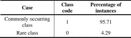
To test the extreme case, we delete 488 instances in the denser class 0 randomly to generate a rare class using the same experimental methods as used in [15, 26, 32, 33]. The class distribution we get is shown in Table 2.

Table 2. The class distribution of Pima Indians diabetes

Case Class

code

Percentage of instances Commonly occurring

class 1 95.71

Rare class 0 4.29

For the NDDOF algorithm, the number of k-neighbor of an object should be larger than the number of the attributes of the dataset, so we select k

equaling 8. For testing the performance of the algorithms with different k values, we also run these algorithms with k equaling 14, 28 and 42, which are the 5%, 10% and 15% of the number of instances in the dataset, respectively. We would not select k to be too large, which will be meaningless for the outlier mining algorithms.

The value of k is 8, which is the size of the attributes, and Table 3 shows the values of recall,

precision and rankpower to measure the performance of the algorithms. The value of m indicates the top m

ranked objects returned by the algorithms. For m = 10, the LOF algorithm, the INFLO algorithm, the

COF algorithm, and the DSNOF algorithm can not find any objects in rare classes while the NDDOF al-gorithm can find one. From m = 20, the NDDOF al-gorithm detects much more outliers than other algori-thms. Moreover, in the top 90 ranked instances, only the NDDOF algorithm mines all instances in the rare class, and the three metrics are always the largest.

For k = 14, the experiment results are shown in Table 4. The LOF algorithm, COF algorithm, INFLO

algorithm and DSNOF algorithm become worse than these algorithms with k = 8, while NDDOF algorithm becomes better. For each m, the NDDOF algorithm with k = 14 detects more outliers than it does with

(7)

Table 3. Detected rare classes in Pima Indians diabetes dataset for k=8

m LOF COF INFLO DSNOF NDDOF

Nrc Pr Re RP Nrc Pr Re RP Nrc Pr Re RP Nrc Pr Re RP Nrc Pr Re RP 10 0 0 0 0 0 0 0 0 0 0 0 0 0 0 0 0 1 0.1 0.1 0.3 20 0 0 0 0 1 0.1 0.1 0.1 1 0.1 0.1 0.1 0 0 0 0 6 0.3 0.5 0.3 30 1 0.1 0.1 0.1 2 0.1 0.2 0.1 3 0.1 0.1 0.1 0 0 0 0 6 0.2 0.5 0.3 40 1 0.1 0.1 0.1 2 0.1 0.2 0.1 3 0.1 0.3 0.1 2 0.1 0.2 0.1 7 0.2 0.6 0.2 50 2 0.1 0.2 0.1 4 0.1 0.3 0.1 3 0.1 0.3 0.1 3 0.1 0.3 0.1 7 0.1 0.6 0.2 60 3 0.1 0.3 0.1 5 0.1 0.4 0.1 3 0.1 0.3 0.1 3 0.1 0.3 0.1 9 0.2 0.8 0.2 70 4 0.1 0.3 0.1 5 0.1 0.4 0.1 3 0.1 0.3 0.1 3 0.1 0.3 0.1 10 0.1 0.8 0.2 80 4 0.1 0.3 0.1 5 0.1 0.4 0.1 4 0.1 0.3 0.1 3 0.1 0.3 0.1 11 0.1 0.9 0.2 90 4 0.1 0.3 0.1 6 0.1 0.5 0.1 4 0.1 0.3 0.1 3 0.1 0.3 0.1 12 0.1 1 0.2

Nrc Pr Re RP Nrc Pr Re RP Nrc Pr Re RP Nrc Pr Re RP Nrc Pr Re RP 10 0 0 0 0 0 0 0 0 0 0 0 0 0 0 0 0 4 0.4 0.3 0.3 20 1 0.1 0.1 0.1 1 0.1 0.1 0.1 0 0 0 0 0 0 0 0 8 0.4 0.7 0.4 30 1 0.1 0.1 0.1 1 0.1 0.1 0.1 1 0.1 0.1 0.1 0 0 0 0 9 0.3 0.8 0.4 40 3 0.1 0.3 0.1 2 0.1 0.2 0.1 2 0.1 0.2 0.1 0 0 0 0 10 0.3 0.8 0.4 50 3 0.1 0.3 0.1 2 0.1 0.2 0.1 2 0.1 0.2 0.1 0 0 0 0 10 0.2 0.8 0.4 60 3 0.1 0.3 0.1 2 0.1 0.2 0.1 2 0.1 0.2 0.1 1 0.1 0.1 0.1 10 0.2 0.8 0.4 70 3 0.1 0.3 0.1 2 0.1 0.2 0.1 2 0.1 0.2 0.1 1 0.1 0.1 0.1 11 0.2 0.9 0.3 80 3 0.1 0.3 0.1 2 0.1 0.2 0.1 3 0.1 0.3 0.1 1 0.1 0.1 0.1 12 0.2 1 0.3

m LOF COF INFLO DSNOF NDDOF

Nrc Pr Re RP Nrc Pr Re RP Nrc Pr Re RP Nrc Pr Re RP Nrc Pr Re RP 10 1 0.1 0.1 0.1 2 0.2 0.2 0.3 2 0.2 0.2 0.3 2 0.2 0.2 0.3 3 0.3 0.3 0.4 20 3 0.2 0.3 0.2 4 0.2 0.3 0.3 3 0.2 0.3 0.2 3 0.2 0.3 0.2 6 0.3 0.5 0.3 30 3 0.1 0.3 0.2 5 0.2 0.4 0.2 4 0.1 0.3 0.2 5 0.2 0.3 0.2 8 0.3 0.8 0.3 40 4 0.1 0.3 0.1 5 0.1 0.4 0.2 4 0.1 0.3 0.2 6 0.2 0.5 0.2 10 0.3 0.8 0.3 50 4 0.1 0.3 0.1 7 0.1 0.6 0.2 5 0.1 0.4 0.2 7 0.1 0.6 0.2 10 0.2 0.8 0.3 60 5 0.1 0.4 0.1 7 0.1 0.6 0.2 7 0.1 0.6 0.1 8 0.1 0.7 0.2 12 0.2 1 0.3

m LOF COF INFLO DSNOF NDDOF

Nrc Pr Re RP Nrc Pr Re RP Nrc Pr Re RP Nrc Pr Re RP Nrc Pr Re RP 10 0 0 0 0 0 0 0 0 1 0.1 0.1 0.1 2 0.2 0.2 0.3 2 0.2 0.2 0.4 20 1 0.1 0.1 0.1 0 0 0 0 1 0.1 0.1 0.1 2 0.1 0.2 0.3 5 0.3 0.4 0.2 30 1 0.1 0.1 0.1 1 0.1 0.1 0.1 3 0.1 0.3 0.1 3 0.1 0.3 0.2 7 0.2 0.6 0.2 40 1 0.1 0.1 0.1 2 0.1 0.2 0.1 4 0.1 0.3 0.1 4 0.1 0.3 0.2 10 0.3 0.8 0.2 50 2 0.1 0.2 0.1 3 0.1 0.3 0.1 4 0.1 0.3 0.1 6 0.1 0.5 0.1 12 0.2 1 0.3

Table 7. The Image segment dataset class distribution

Case Class code Percentage of instances

(8)

Table 8. Detected rare classes in Image segment dataset for k=19

Nrc Pr Re RP Nrc Pr Re RP Nrc Pr Re RP Nrc Pr Re RP Nrc Pr Re RP

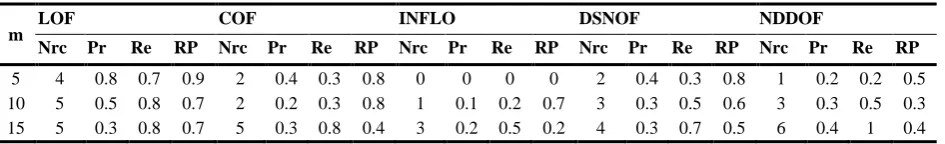
5 4 0.8 0.7 0.9 2 0.4 0.3 0.8 0 0 0 0 2 0.4 0.3 0.8 1 0.2 0.2 0.5 10 5 0.5 0.8 0.7 2 0.2 0.3 0.8 1 0.1 0.2 0.7 3 0.3 0.5 0.6 3 0.3 0.5 0.3 15 5 0.3 0.8 0.7 5 0.3 0.8 0.4 3 0.2 0.5 0.2 4 0.3 0.7 0.5 6 0.4 1 0.4

Nrc Pr Re RP Nrc Pr Re RP Nrc Pr Re RP Nrc Pr Re RP Nrc Pr Re RP 5 4 0.8 0.7 1 2 0.4 0.3 1 1 0.2 0.2 0.3 2 0.4 0.3 0.5 4 0.8 0.7 1 10 5 0.5 0.8 0.6 3 0.3 0.5 0.2 3 0.3 0.5 0.3 3 0.3 0.5 0.3 5 0.5 0.8 0.8 15 5 0.3 0.8 0.6 5 0.3 0.8 0.4 4 0.2 0.5 0.3 5 0.3 0.7 0.4 6 0.4 1 0.4

Nrc Pr Re RP Nrc Pr Re RP Nrc Pr Re RP Nrc Pr Re RP Nrc Pr Re RP 5 4 0.8 0.7 1 2 0.4 0.3 1 3 0.6 0.5 0.6 2 0.4 0.3 0.4 5 1 0.8 1 10 5 0.5 0.8 0.6 5 0.5 0.8 0.5 3 0.3 0.5 0.4 3 0.3 0.5 0.3 5 0.5 0.8 1 15 5 0.3 0.8 0.6 5 0.3 0.8 0.5 4 0.3 0.7 0.5 4 0.3 0.7 0.3 6 0.4 1 0.8

For k = 28 and k = 42, the experiment results are shown in Table 5 and Table 6 which are almost consistent with Table 3 and Table 4. The algorithms perform better than those with k equaling 8 and 14. For each m, the Nrc, Pr, Re and RP returned by

NDDOF are larger than those returned by other algo-rithms. As the extreme case is tested, the values of

Pr, Re and RP returned by the algorithms are small, but the NDDOF algorithm performs better on this dataset.

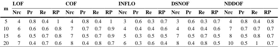
4.3.2. Image segment dataset

The second real UCI dataset is Image segment dataset. A total of 210 instances with 19 attributes is divided into seven classes with the same size. The seven classes are named sky, brickface, foliage, win-dow, cement, grass, and path, respectively.

Following the same approach as in [15, 26, 32, 33] , we randomly select 2 classes to form rare classes and other 2 classes as small cluster classes. The rest of 3 classes form the commonly occurring classes. Table 7 lists the class distribution of the dataset.

We perform the LOF algorithm, the INFLO

algorithm, the COF algorithm, the DSNOF algorithm and the NDDOF algorithm on this dataset to find the rare classes. The values of k are 19, 23 and 30, which are the size of the attribute, the 30% and 40% of the number of the instances, respectively. The experiment results are listed in Tables 8 to 10.

For k = 19, in the top 5 ranked objects detected by each algorithm, all of the algorithms except the

INFLO algorithm are more effective than the

NDDOF algorithm in terms of the Nrc, Re, Pr, and

RP. For m=10, the Nrc of NDDOF algorithm is 3 which is smaller than that of LOF algorithm and equal to that of DSNOF algorithm. But the Nrc of

NDDOF algorithm is larger than the Nrc of the COF

algorithm and that of INFLO algorithm. Among the top 15 ranked records, only the NDDOF algorithm finds all the outliers. Although the RP of NDDOF

algorithm is 0.4 which is smaller than that of LOF

algorithm and that of DSNOF algorithm, Re and Pr

returned by NDDOF algorithm are always the largest. For k = 23, both the NDDOF algorithm and the

LOF algorithm can detect the top 4 objects as outliers. For m = 10, the NDDOF algorithm and the

LOF algorithm can find 5 outliers, but the RP

returned by NDDOF algorithm is larger. When m = 15, only the NDDOF algorithm can detect 6 outliers.

For k = 30, the top 5 objects ranked by NDDOF

algorithm are outliers, while LOF algorithm detects the top 4 objects as outliers. For m = 10, both the

NDDOF algorithm and the LOF algorithm can detect 5 outliers, but the RP returned by LOF algorithm is smaller. When m = 15, only the NDDOF algorithm can detect 6 outliers, which is similar to the results for k = 23.

4.3.3. Ionosphere dataset

(9)

Table 11 shows the class distribution of the data-set. We run the LOF algorithm, the INFLO algorithm, the COF algorithm, the DSNOF algorithm and the

NDDOF algorithm on the dataset to find the rare class. We chose k being 34, 47 and 59, which are the size of the attributes, 20% and 25% size of the data-set, respectively. The results are shown in Tables 12 to 14.

Table 11. The Ionosphere class distribution

Case Class code Percentage of instances

Commonly occurring class Good 95.74

Rare class Bad 4.26

For k = 34, among the top 5 ranked instances detected by the algorithms, the NDDOF algorithm can detect 4 rare instances which is only one less than that detected by the COF algorithm and the RP is smaller than the RP of LOF algorithm. However, for

m being from 10 to 15, the NDDOF algorithm perfor-ms better than the other algorithperfor-ms, although the rank power of NDDOF algorithm is smaller than that of

COF algorithm. For m = 20 the NDDOF algorithm can detect all 10 rare instances while the LOF algo-rithm can detect 9 rare instances and the INFLO only detects 6 rare instances. The RP of NDDOF is 0.8 which is larger than that of other algorithms.

For k = 47, the LOF algorithm performs better than the NDDOF algorithm when m = 5, because although the LOF algorithm and the NDDOF

algori-thm can detect 4 outliers in top 5 ranked objects, the

RP returned by LOF is 1 which is larger than that of

NDDOF algorithm. Even more, the COF algorithm can detect the top 5 objects as outliers, which is also better than the NDDOF algorithm. With the value of

m increasing from 10 to 20, the NDDOF algorithm detects more outliers than other algorithms do. Such as for m = 15, the NDDOF algorithm can detect 9 outliers while DSNOF algorithm detects 6 outliers.

For k = 59, the LOF algorithm, the COF algo-rithm and the NDDOF algorithm can detect 4 outliers when m = 5, and the RP returned by NDDOF algo-rithm is smaller than that returned by the LOF algo-rithm and by the COF algorithm. For m = 10, both the NDDOF algorithm and the COF algorithm can detect 7 outliers, and the RP returned by NDDOF

algorithm is smaller. However, for m being 15 to 20, the NDDOF algorithm could detect more rare instan-ces than the LOF algorithm, the INFLO algorithm, the COF algorithm and the DSNOF algorithm do. Furthermore, among top 20 ranked instances returned by the algorithms, only the NDDOF algorithm detects all instances in rare class.

From the experiments on the three real datasets, the NDDOF algorithm performs better than the LOF

algorithm, the INFLO algorithm, the COF algorithm, and the DSNOF algorithm with different k values. For convenience, we could choose k being equal to the number of dimensions d. The results of experi-ments also show that the NDDOF algorithm could be adopted in practice.

Table 12. Detected rare classes in Ionosphere dataset for k=34

5 4 0.8 0.4 0.9 5 1 0.5 1 3 0.6 0.3 0.8 2 0.4 0.2 1 4 0.8 0.4 0.8 10 6 0.6 0.6 0.8 6 0.6 0.6 1 6 0.6 0.6 0.6 5 0.5 0.5 0.6 8 0.8 0.8 0.9 15 7 0.5 0.7 0.7 6 0.4 0.6 1 6 0.4 0.6 0.6 6 0.4 0.6 0.6 9 0.6 0.9 0.8 20 7 0.4 0.7 0.7 9 0.5 0.9 0.4 6 0.3 0.6 0.6 7 0.4 0.7 0.5 10 0.5 1 0.8

m

LOF COF INFLO DSNOF NDDOF

5 4 0.8 0.4 1 5 1 0.5 1 4 0.8 0.4 0.7 3 0.6 0.3 1 4 0.8 0.4 0.9 10 5 0.5 0.5 0.8 6 0.6 0.6 0.9 5 0.5 0.5 0.7 4 0.4 0.4 0.8 7 0.7 0.7 0.8 15 6 0.4 0.6 0.7 6 0.4 0.6 0.9 5 0.3 0.5 0.7 6 0.4 0.6 0.5 9 0.6 0.9 0.8 20 7 0.4 0.7 0.6 9 0.5 0.9 0.6 6 0.3 0.6 0.5 7 0.4 0.7 0.5 10 0.5 1 0.7

Nrc Pr Re RP Nrc Pr Re RP Nrc Pr Re RP Nrc Pr Re RP Nrc Pr Re RP

(10)

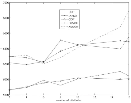
Figure 5. Running time of the algorithms with instances changing for k=16

Figure 6. Running time of the algorithms with different attributes for k=16

4.4. Time performance and scalability

In this section, we evaluate the time performance and the scalability of the LOF algorithm, the INFLO

algorithm, the COF algorithm, the DSNOF algorithm and the NDDOF algorithm with the same method as in [27]. The test dataset is also a UCI dataset, named letter-recognition dataset. The dataset has 20000 instances with 16 attributes.

With increasing number of instances from 2000 to 10000, Figure 5 shows the running time of each algorithm on the dataset with 16 attributes and k = 16. Obviously, the time complexity of NDDOF algorithm is higher than that of others. It is because getting the minimum hyper sphere is an iterative process that the density calculating progress costs much time.

When the number of instances becomes larger than 8000, the running times of these algorithms are similar, namely, the time growth rate of NDDOF is smaller than others.

To evaluate the scalability of the algorithms about the dimension of the dataset, we run the five algorithms on the letter-recognition dataset with 8000 instances and the number of attributes increasing from 2 to 16. The results are exhibited in Figure 6. The

running time of five algorithms doesn’t change much. In other words, the number of attributes has little effect on the scalability of the algorithms.

5. Conclusions

This paper presents a neighbor-density-deviation based outlier detecting algorithm.

For verifying the effectiveness of the new density definition, we conducted experiments on a synthetic dataset. Furthermore, we also experiment with the

NDDOF algorithm on real UCI datasets. The results demonstrate some advantages of our algorithm. First, the parameter k of NDDOF algorithm could be chosen easily, and is generally equal to the number of dimension of the dataset. The value of k will reduce the subjective influence to the algorithm. Second, our density definition of an object is more proper and meaningful than the existing definitions. Third, the

NDDOF algorithm can deal with a dataset with different density clusters. Fourth, the NDDOF

algorithm could distinguish outliers from the objects in the small cluster correctly. Even more, the proposed outlier detecting algorithm is more accurate than the existing algorithms.

Because the time complexity of NDDOF is high, the future research work will focus on improving the time performance of our algorithm by using the R-tree and distributed computing.

Acknowledgments

The research is financially supported by the National Natural Science Foundation of China (61375055), the Program for New Century Excellent Talents in University (NCET-12-0447), the Natural Science Foundation of Shaanxi Province of China (2014JQ8365) and the Fundamental Research Funds for the Central University.

References

[1] D. Hawkins. Identification of Outliers. London: Chapman and Hall, 1980.

[2] K. Shi, L. Li. High performance genetic algorithm based text clustering using parts of speech and outlier elimination. Applied Intelligence, 2013, Vol. 38, No. 4, 511-519.

[3] A. S. Koyuncugil, N. Ozgulbas. Financial early warning system model and data mining application for risk detection. Expert Systems with Applications, 2012, Vol. 39, No. 6, 6238-6253.

[4] P. Chaste, L. Klei, S. J. Sanders, et al. Adjusting Head Circumference for Covariates in Autism: Clinical Correlates of a Highly Heritable Continuous Trait. Biological Psychiatry, 2013, Vol. 74, No. 8, 576-584. [5] K. Zhang, M. Luo. Outlier-robust extreme learning

(11)

[6] H. Zhao, B. Jiang, J. Tang, B. Luo. Image matching using a local distribution based outlier detection technique. Neurocomputing, 2015, Vol. 148, 611-618. [7] R. Y. Jiang, H. L. Fei. A Family of Joint Sparse PCA

Algorithms for Anomaly Localization in Network Data Streams. IEEE Transactions on Knowledge and Data Engineering, 2013, Vol. 25, Issue 11, 2421-2433. [8] V. Barnett, T. Lewis. Outliers in Statistical-Data.

Journal of the Operational Research Society, 1995, Vol. 46, Issue 8, 1034-1035.

[9] V. J. Hodge, J. Austin. A survey of outlier detection methodologies. Artificial Intelligence Review, 2004, Vol. 22, No. 2, 85-126.

[10] Hido, T. Y. Inlier-based outlier detection via direct density ratio estimation. In: The 8th IEEE International Conference on Data Mining, Washington DC, USA, 2008, pp. 223-232.

[11] M. E. Otey, A. Ghoting, S. Parthasarathy. Fast distributed outlier detection in mixed-attribute data sets. Data Mining and Knowledge Discovery, 2006, Vol. 12, No. 2-3, 203-228.

[12] K. Yamanishi, J.-I. Takeuchi. Discovering outlier filtering rules from unlabeled data. In: Proceedings of the 7th ACM SIGKDD International Conference on Knowledge discovery and data mining, New York, USA, 2001, pp. 389-394.

[13] C. Cassisi, A. Ferro, R. Giugno. Enhancing density-based clustering: Parameter reduction and outlier detection. Information Systems, 2013, Vol. 38, No. 3, 317-330.

[14] L. Duan, L. Xu, F. Guo. A local-density based spatial clustering algorithm with noise. Information Systems, 2007, Vol. 32, No. 7, 978-986.

[15] P.-N. Tan, M. Steinbach, V. Kumar. Introduction to data mining. USA: Addison-Wesley Higher Education, 2006.

[16] E. M. Knorr, R. T. Ng. Algorithms for mining distance-based outliers in large datasets. In: Proceedings of the 24th International Conference on Very-Large Databases, New York, USA, 1998, pp. 392-403.

[17] E. Knorr, R. Ng, V. Tucakov. Distance-based outlier: Algorithms and applications. The VLDB Journal, 2000, Vol. 8, No. 3, 237-253.

[18] F. Angiulli, S. Basta. Distributed Strategies for Mi-ning Outliers in Large Data Sets, IEEE Transactions on Knowledge and Data Engineering, 2013, Vol. 25, No. 7, 1520-1532.

[19] M. M. Breunig, H. P. Kriegel. LOF: Identifying density-based local outliers. ACM SIGMOD Record, 2000, Vol. 29, No. 2, 93-104.

[20] J. Wen, Anthony, K. H. Tung, J. Han. Mining top-n local outliers in large databases. In: Proceedings of the

7th ACM SIGKDD International Conference on Knowledge Discovery and Data Mining, New York, USA, 2001, pp. 293-298.

[21] A. L. M. Chiu, W.-F. Ada. Enhancements on local outlier detection. In: Proceedings of the 7th International Database Engineering and Applications Symposium, Sigmod Record, 2003, pp. 298–307. [22] S. Papadimitriou, H. Kitawaga, P. B. Gibbons, C.

Faloutsos. LOCI: Fast outlier detection using the local correlation integral. In: The 19th International Conference on Data Engineering, Bangalore, India 2003, pp. 315–328.

[23] J. Tang, Z. X. Chen, A. W. C. Fu, et al. Capabilities of outlier detection schemes in large datasets, framework and methodologies. Knowledge and Information Systems, 2007, Vol. 11, No. 1, 45-84. [24] W. Jin, A. K. H. Tung, J. W. Han, W. Wang.

Ranking outliers using symmetric neighborhood relationship. Lecture Notes in Computer Science, 2006, Vol. 3918, pp. 577-593.

[25] Y. Wan, F. Bian. Cell-based outlier detection algorithm, In: the 12th Pacific-Asia Conference on Knowledge Discovery and Data Mining, Osaka, Japan, 2008, pp. 1042–1048.

[26] F. Jiang, Y. F. Sui, C. G. Cao. Some issues about outlier detection in rough set theory. Expert Systems with Applications, 2009, Vol. 36, No. 3, 4680-4687. [27] H. Cao, G. Q. Si, Y. B. Zhang, L. Jia. Enhancing

effectiveness of density-based outlier mining scheme with density-similarity-neighbor-based outlier factor. Expert Systems with Applications, 2010, Vol. 37, No. 12, 8090-8101.

[28] http://en.wikipedia.org/wiki/N-sphere.

[29] P. Kumar, J. Mitchell, E. Yildirim. Computing Core-Sets and Approximate Smallest Enclosing HyperSpheres in High Dimensions. In: 5th Workshop on Algorithm Engineering and Experiments (ALENEX 2003) BALTIMORE, MD, 2003, pp. 45-55.

[30] X. Meng, Z. Chen. On user-oriented measurements of effectiveness of web information retrieval systems, In: International Conference on Internet Computing/International Symposium on Web Services and Applications, Las Vegas, USA, 2004, pp. 527-533. [31] C. C. Aggarwal, P. S. Yu. Outlier detection for high dimensional data. ACM SIGMOD Record, 2001, Vol. 30, No. 2, 37-46.

[32] M. Ye, X. Li, M. E. Orlowska. Projected outlier detection in high-dimensional mixed-attributes data set. Expert Systems with Applications, 2009, Vol. 36, No. 3, 7104-7113.

[33] Z. Y. He, X. F. Xu, S. C. Deng. Discovering cluster-based local outliers. Pattern Recognition Letters, 2003, Vol. 24, Issue 9-10, 1641-1650.