39
*Corresponding author
Email address: [email protected]
Optimization of the injection molding process of Derlin 500 composite
using ANOVA and grey relational analysis
S. Khalilpourazarya,* and N. Payamb
a Faculty of Mechanical Engineering, Urmia University of Technology, Urmia, Iran
b Projects Engineering Department, Mapna Boiler & Equipment Engineering & Manufacturing Co., Karaj, Iran
Article info: Abstract
Warpage and shrinkage control are important factors in proving the quality of thin-wall parts in injection modeling process. In the present paper, grey relational analysis was used in order to optimize these two parameters in manufacturing plastic bush of articulated garden tractor. The material used in the plastic bush is Derlin 500. The input parameters in the process were selected according to their effect on shrinkage and warpage values, melt temperature, mold temperature, injection rate, injection pressure, and packing pressure. Then, the Taguchi method was applied to design the experiments, and through the use of Mold Flow software injection molding process was simulated based on these experiments and the input parameters. Based on the results obtained from the simulation, the input parameters were analyzed in three levels using grey relational analysis. Then, analysis of variance and confirmation tests were carried out on the output of grey relational analysis to predict the optimum values of the input parameters and to calculate the dimensional changes of the plastic bush. Gaining these values, the plastic bush sample was manufactured, and its 3D point cloud model was generated by a scanner. At the end, by generating 3D solid model of the plastic bush its dimensional features were studied. The comparison of the warpage and shrinkage values between grey relational analysis and 3D CAD model indicates the precision of the method in controlling and measuring these two parameters.
Received: 18/02/2015 Accepted: 08/03/2016 Online: 11/09/2016
Keywords:
Injection molding, Grey Relational Analysis, ANOVA,
Warpage, Shrinkage.
1. Introduction
Injection molding process is a conventional manufacturing method for producing parts by injecting material into a metal mold. One of the advantages of this method is the possibility of manufacturing plastic parts with thin-wall plastics. The quality of the manufactured parts depends on the plastic material, the design of
40
shrinkage in the part. Based on the studies carried out, the low injection pressure, low cooling time, high temperature of the melt and the mold, the low packing pressure, and dissimilar cooling are among chief factors of shrinkage [2]. On the other hand, the geometry of the part and the mechanical properties of the material are very effective factors in the phenomenon of warpage. According to the importance of controlling these defects in plastic parts, a lot of studies have been carried out on the effective and controllable parameters in injection modeling process. Lioa et.al [2] employed the Taguchi method to measure warpage and shrinkage of the thin-wall injected parts. Based on the studies, packing pressure has the most effective role in warpage and shrinkage in thin-wall parts.
Shen et.al [3] simultaneously used grey relational analysis and Taguchi method to study the effect of input parameters like injection temperature, mold temperature, injection time, injection pressure, on microinjection modeling in PMO, PS, PC, PP plastics. The investigations reveal that the ability to predict the optimum value of the input parameters in grey relational analysis method is highly compatible with the results obtained from Mold Flow software. In another study, the orthogonal array with the grey relational analysis and Fuzzy logic analysis was used in injection molding process of parts with PS/ABS material to optimize the parameters of mold temperature, melt temperature, filling pressure, and filling time. The results from the experiments showed that using the methods at the same time can greatly increase the productivity of manufacturing [4]. Tang et.al [5] studied the factors effective in reducing warpage using the Taguchi method. The results indicated that melt temperature and filling time respectively have the highest and the lowest effects on the warpage in plastic parts. Based on this, to decrease warpage, the optimum values for melt temperature, packing pressure, packing time, and filling time were presented. Oktem et.al [6] used the signal-to-noise (S/N) and the analysis of variance (ANOVA) to optimize shrinkage and warpage values for thin-shell parts and proved the efficiency of this method [7]. In the present
paper, the injection molding process in plastic bush of the articulated garden tractor was investigated. The Taguchi method was used to design the experiments, and the injection molding process was simulated by Mold Flow software. Based on this simulation, we obtained the levels needed to predict optimum values for the input parameters and the amount of dimensional changes in the plastic bush by integrating grey relational analysis and ANOVA. Based on these results, the sample plastic bush was manufactured. Then, the bush was scanned by DL-SET01 scanner and a 3D CAD model of the bush was generated from its 3D point cloud model.
2. The properties of the plastic bush
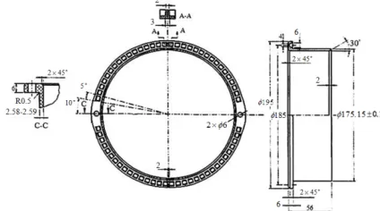
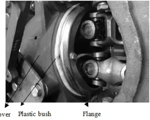
The plastic bush used in the present study assembled between the flange and cover in the articulation central of the tractor. It made motion possible in these two parts and makes it possible in the tractor that the flange of the articulation center rotates in the cover with at last 15while moving across unequal surfaces. The plastic bush drawing along with the dimensions (in millimeters) is depicted in Fig. 1.
Fig. 1. Dimensions of the selected plastic bush (in millimeters).
41
Fig. 2. Plastic bush assembled between cover and flange in the articulation central of the tractor.
Fig. 3. Generated fracture in plastic polyethylene bush.
3. The change in the material of the plastic bush
According to the inefficiency of polyethylene, for this purpose, another material was chosen to substitute it. In this study, Derlin 500, which is one of the engineering thermoplastics, has been used. Low friction coefficient, excellent dimensional stability, resistance against high wear, and its use in precision parts requiring high stiffness are some of the properties of Derlin 500. The physical properties of Derlin 500 plastic to manufacture a plastic bush are presented in table 1.
After deciding for the material of the plastic bush, its 3D CAD model was provided according to the depicted dimensions in Fig. 1. To analyze the molding injection process of the plastic bush, and also to design gate, runner and sprue, and the cooling system of the mold Mold Flow software was used. Then, using the results from the simulation, the injection process of adequate range for, five parameters melt temperature (Me), mold temperature (Mdie
), injection rate (IR), injection pressure (
p
P ),
and package pressure (Ppp), were determined.
Figure 4 shows the analysis of plastic bush of the articulation central in this software using Derlin 500 material.
Table 1. Physical characteristics of Derlin 500. Value Parameter
3530-3550 MPa Elastic Modulus
0.38-0.42 Poisson's Ratio
1360 MPa Shear Modulus
0.0001
C
1
CTE
1500-2000
C Kg.
J
Specific Heat
0.3-0.23 mc
W Thermal Conductivity
1.1494
3
cm g Melt Density
1.435 3
cm g
Solid Density
(50C-105C) Mold Temperature
(180C-235C) Melt Temperature
118 C Ejection Temperature
0.45 MPa Max. Shear Stress
40000
S
1
Max. Shear Rate
Fig. 4. Simulation of the injection molding process in Mold Flow software.
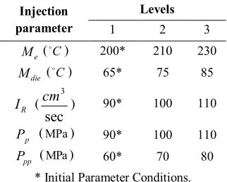
4. Levels of the experiment
42
objectives, unlike the difficulties and infeasibility of other methods. In grey analysis, each test has input parameters divided into levels according to the application conditions or the effectiveness. In this study, according to the analysis in the Mold Flow software, five input parameters for the plastic injection molding process were selected and investigated in three levels. The parameters and the levels under investigation are shown in table 2, and all the experiments are according to the defined levels [8]. Level one is considered the primary parameter for all the parameters.
5. Orthogonal array
These arrays are
m
n
matrixes with the rows as the number of tests and columns as the input parameters. The matrix is built in the way that repeating tests are identified while the experiments are carried out to satisfy the minimum number of tests such that the final target can be achieved. The total degree of freedom for the proposed system is calculated as follows [9]:(5.1) FD =1+
(Degree of Freedom×level)Table 2. Parameters and related levels. Injection
parameter
Levels
1 2 3
e
M (C) 200* 210 230
die
M (C) 65* 75 85
R
I (
sec
3
cm
) 90* 100 110
p
P (MPa) 90* 100 110
pp
P (MPa) 60* 70 80
* Initial Parameter Conditions.
Since the degree of freedom for this system is 11, the array L27can be used due to the capability of the array in designing the specific type of the experiment.
6. The considered positions on the plastic bush geomtry
The amount of warpage and shrinkage in a plastic part can be studied in different points of that. In this paper, to determine the values for warpage and shrinkage in the plastic bush, the very points were used which are important in the geometry of the part and its assembly inside the articulation central. The defined positions for the values of
x
1,x
2,x
3,x
4,x
5,y and z on the plastic bush are shown in Fig. 5.By determining these points, the amount of shrinkage in points
x
1,x
2,x
3,x
4,x
5 are respectively shown by x1,x2,x3,x4, and5
x
. Shrinkage along
x
axis is defined in Eq. (6.1).(6.1) ) (
5 1
5 4 3 2
1 x x x x
x
X
Fig. 5. Considered positions on the plastic bush geometry.
Shrinkage along y axis is shown by Y and is calculated from the following equation:
(6.2) Y
Y
Warpages along
z
axis are measured by determining displacement alongz
axis for pointsz
1 andz
2. In the present paper warpageis defined as out of plane deformation with transitional reference plane from point
z
2. Ininjected plastic bush the amount of warpage in
43
2
Z
respectively, and in this case the amount of warpage in
z
direction are measured through Eq. (6.3). (6.3) 2 1 Z ZZ
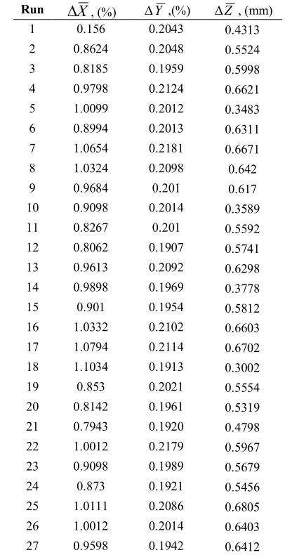
So, the values measured for the warpage along z axis and the shrinkages along x and y for all the experiments by Mold Flow software is presented in table 3.
7. Grey relational analysis
Grey relational analysis was first suggested by J. Deng in 1982 [10]. The purpose of grey relational analysis is to change an issue to a simple and comprehensible one. To this end, inputs with multiple objectives are turned to inputs with one objective so that getting the results and analyzing inputs are simplified after normalizing them by grey relational generating and obtaining grey relational coefficient and grey relational grade.
Then based on these the grey graph is drawn. So, in order to make comparison possible, first the parameters should be made normalized so the process of comparing them makes sense [10]. Since the lower the values for warpage and shrinkage, the better the quality of the part manufactured, Eq. (7.1) is used to normalize and make grey relational generating.
(7.1) ) ( min ) ( max ) ( ) ( max )
( 0 0
0 0 * k X k X k X k X k X i i i i i
In this equation,
max
X
i0(
k
)
is the largest value ofX0(k)i , min ( ) 0
k
Xi is the smallest value of
X
i0(
k
)
andX
i*(
k
)
parameters is the input value of grey relational analysis for the i response for the k experiment, which is the crude value of the input prior to analysis [10]. To provide a great understanding of grey relational generating, a value is defined as the difference of the input value which can be compared from Eq. (7.2) [11].(7.2) ) ( ) ( ) ( * * 0
0i k X k Xi k
To determine grey relational coefficient, Eq. (7.3) is employed [11, 12]
(7.3) max 0 max min . ) ( . ) ( k k i i
Table 3. Numerical layouts obtaining from Mold Flow simulation.
Run X, (%) Y ,(%) Z , (mm)
1 0.156 0.2043 0.4313
2 0.8624 0.2048 0.5524
3 0.8185 0.1959 0.5998
4 0.9798 0.2124 0.6621
5 1.0099 0.2012 0.3483
6 0.8994 0.2013 0.6311
7 1.0654 0.2181 0.6671
8 1.0324 0.2098 0.642
9 0.9684 0.201 0.617
10 0.9098 0.2014 0.3589
11 0.8267 0.201 0.5592
12 0.8062 0.1907 0.5741
13 0.9613 0.2092 0.6298
14 0.9898 0.1969 0.3778
15 0.901 0.1954 0.5812
16 1.0332 0.2102 0.6603
17 1.0794 0.2114 0.6702
18 1.1034 0.1913 0.3002
19 0.853 0.2021 0.5554
20 0.8142 0.1961 0.5319
21 0.7943 0.1920 0.4798
22 1.0012 0.2179 0.5967
23 0.9098 0.1989 0.5679
24 0.873 0.1921 0.5456
25 1.0111 0.2086 0.6805
26 1.0012 0.2014 0.6403
27 0.9598 0.1942 0.6412
In which the parameter min, max, 0i(k), )
(k
i
44
the i response for the k experiment, grey coefficient, respectively. It should be noticed that the value of the grey coefficient is restricted to the range [0, 1] and according to the reference [12], the optimal grey coefficients are usually selected as average (0.5).
8. Grey relational grade
Grey relational grade, along with grey relational coefficient, is a parameter which helps clarifying the input position to obtain an optimal response. This parameter is obtained through Eq. (8.1) [12].
(8.1)
m
k i i
i k
m 1
) ( 1
where,
iis the weighted value or importance of each parameter. When all the parameters have the same level of effectiveness,
ican be neglected. Table 4 lists the related grey relational grade for each grey relational coefficient.Equation (8.2) can use to determine the grey relational grade for each level. It is obvious that grey relational grade for each level is the average amount of all grades [13].
(8.2)
k
i i
k
A
1
1
Where,
A
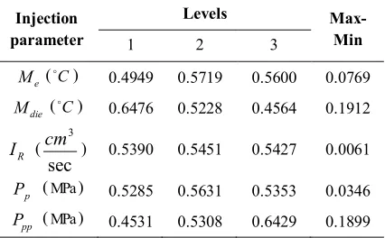
indicates grey grade for each level and k is a constant coefficient [14].Table 5 includes grey relational grade for each level. In this table, a set of values is presented as Max-Min values for grey grade data; these values are indeed the difference between the maximum and the minimum values of grey grade for each level. This value shows the stability of each parameter. The lower it is, the more stable the parameter is.
9. Grey relational graph
Grey relational graph is related to the levels and grey relational grade for each level; it is first determined as points, then the line crossing
these points is drawn. In this paper grey relational graph for each level is studied and then drawn according to the tables for each level (see Fig. 6); finally, all five graphs are presented in one graph [15, 16].
Table 4. Grey relational coefficient and grey relational grade.
Run
Grey relational
coefficient Grey
relational grade
Order X
, %
Y
, %
Z
, mm
1 0.560 0.502 0.592 0.551 15
2 0.694 0.493 0.430 0.539 13
3 0.865 0.725 0.388 0.659 22
4 0.454 0.387 0.344 0.395 7
5 0.418 0.566 0.798 0.594 18
6 0.595 0.564 0.365 0.508 11
7 0.363 0.333 0.341 0.346 1
8 0.394 0.418 0.357 0.390 5
9 0.470 0.571 0.375 0.472 10
10 0.572 0.561 0.764 0.633 21
11 0.827 0.571 0.423 0.607 19
12 0.929 1.000 0.410 0.779 26
13 0.481 0.425 0.366 0.424 8
14 0.442 0.688 0.710 0.613 20
15 0.592 0.745 0.404 0.580 17
16 0.393 0.413 0.346 0.384 3
17 0.352 0.398 0.339 0.363 2
18 0.333 0.958 1.000 0.764 25
19 0.725 0.546 0.427 0.566 16
20 0.886 0.717 0.451 0.685 24
21 1.000 0.913 0.514 0.809 27
22 0.428 0.335 0.391 0.384 4
23 0.572 0.626 0.415 0.538 12
24 0.663 0.907 0.437 0.669 23
25 0.416 0.434 0.333 0.394 6
26 0.428 0.561 0.359 0.449 9
27 0.483 0.797 0.358 0.546 14
Table 5. Grey relational grade for each level.
Injection parameter
Levels
Max-Min
1 2 3
e
M (C) 0.4949 0.5719 0.5600 0.0769
die
M (C) 0.6476 0.5228 0.4564 0.1912
R
I (
sec
3
cm
) 0.5390 0.5451 0.5427 0.0061
p
P (MPa) 0.5285 0.5631 0.5353 0.0346
pp
45
Fig. 6. Effect of injection molding parameter levels on the multi-performance.
10. Value of effectiveness of each parameter
The calculation of the influence of each parameter can be done by Eqs. (10.1) to (10.4) [17].
(10.1)
k
i ij
K B
1
1
(10.2)
n m k
(10.3) 100
1
m
i ij ij i
B N
B N B
(10.4) )
( ij ij
ij Max Min
B
N
where,B is the grey grade for each parameter,
ij
is the grey relational coefficient, k is the equation coefficient, m is the number of tests with level value of n,B
i is the ith parameter effectiveness percent for jth level andN
B
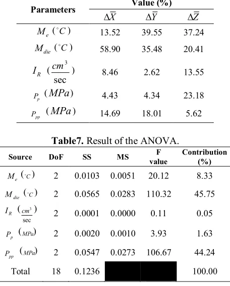
ijisthe Max-Min value of grey relational coefficient for each level. Table 6 lists the effectiveness values of input parameters on the results.
11. Analysis of variance
The final goal in Analysis of Variance is to study the effects of parameters injection molding process on the properties of the final manufactured part. This is done through total
variability of grey relational grades. The total variability is determined from the sum of squared deviations of the total mean of the grey relational grade by each input parameter and the error. In ANOVA, Fisher’s ratio is used to determine whether a parameter has a considerable effect on quality characteristic or not. This process is possible by comparing the F value of the test of each parameter with the standard F value (F0.05) at the 5 % significance level. If the F value is greater than F0.05, then the parameter under investigation has a significant effect on the process [18]. Also, the percentage of each parameter’s contribution in the total sum of the squared deviations can be used to study the importance of each parameter’s change involved in the process [18]. The more the F value increases, the more its effect on the performance of the process is [19]. In the present study, errors are ignored due to their inconsiderable effect. In table 7, the results from ANOVA are presented.
Table 6. Effectiveness values of input parameters on plastic bush geometry.
Value (%) Parameters
Z
Y
X
37.24 39.55
13.52
e
M (C)
20.41 35.48
58.90
die
M (C)
13.55 2.62
8.46
R
I (
sec
3
cm )
23.18 4.34
4.43
p
P (MPa)
5.62 18.01
14.69
pp
P (MPa)
Table7. Result of the ANOVA.
Source DoF SS MS F
value
Contribution (%)
e
M (C) 2 0.0103 0.0051 20.12 8.33
die
M (C) 2 0.0565 0.0283 110.32 45.75
R
I (
sec
3
cm ) 2 0.0001 0.0000 0.11 0.05
p
P (MPa) 2 0.0020 0.0010 3.93 1.63
pp
P (MPa) 2 0.0547 0.0273 106.67 44.24
46
12. Confirmation test
According to the results presented in table 5, in this phase the confirmation test Eq. (12.1) is used to estimate grey relational grade and each output parameter [20].
) (
1
1 m n
k
m
(12.1)
In this equation,
m is the grey relational grade average for each level,
1 is the optimal grey relational grade for each level, and n is the number of input parameters. The estimation of grey relational grade means the average of grey relational grade values added to the total difference between optimal grey relational grade for each level and the mean for the optimal parameters; this is presented in table 8.Table 8. Results of Parameters Effectiveness. Initial
parameter setting
Optimal parameters
Prediction Experime nt
Level Me1Mdie1 IR1PP1PPP1
Me3Mdie1
IR3PP2PPP3
Me2Mdie1
IR2PP2PPP3
ΔX 0.9156 0.7867 0.7943
ΔY 0.2043 0.1902 0.1920
ΔZ 0.4313 0.4752 0.4798
GRG 0.6922 0.8014 0.8092
Improvement in grey relational grade: 0.1170
In this table, the Initial Parameter Setting row is about the initial setting and the basic experiment. The Experiment row is calculated based on the experiment results which are included in table 3, and the Prediction row is about the predictions of the practical results which are very close to experiment results. Grey relational grade in the most optimal experiment shows an increase of 0.1170 units, and this is an indication of total optimal experiment situation.
13. Manufacturing of the injection mold
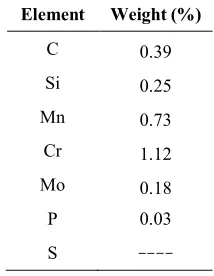
According to plenty number of plastic bushes manufactured, steel Mo40 is used to manufacture the mold. Some properties of this steel include sufficient plasticity, durability, yield strength, tensile strength, good thermal conductivity, and anti-corrosion qualities. In tables 9 and 10 the chemical composition of this steel and equivalent steels in other standards are show.
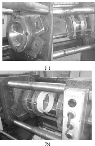
To manufacture molds electro discharge machining operation (EDM) and milling are applied on plates made of Mo40. 5 Axis CNC milling machine model Fanuc was used for milling the mold. Figure 7(a) shows the injection mold manufactured based on the analyses on the plastic bush in Mold Flow software, and Fig. 7(b) shows the manufactured plastic bush after the injection process.
Table 9. The percentages of the steel Mo40 components.
Element Weight (%)
C 0.39
Si 0.25
Mn 0.73
Cr 1.12
Mo 0.18
P 0.03
S
----Table 10. The equivalents of steel Mo40 in different standards.
Germany DIN U.S.A
SAE/ASTM Sweden
S.S. England
B.S.
Standard
1.7225 4140
42CrMo4 708M40
Steel name
14. 3D scanning process
47 (a)
(b)
Fig. 7. (a) Manufactured mold inserted on the injection machine, (b) Mnufactured plastic bush.
Fig. 8. 3D point cloud model of manufactured plastic bush.
3D scanner measures a vast number of points on external surface of a workpiece and output results consist of a point cloud as a data file. 3D point cloud is a collection of the points that usually defined by X, Y, and Z coordinates in a three-dimensional coordinate system and often represent the external surface of a scanned object. Point clouds can be directly inspected, but usually are not directly usable in most 3D
applications. Therefore a common way is to convert the 3D point cloud to a CAD model through a process named surface reconstruction. In this paper, by 3D point cloud model, 3D CAD model was produced and all its dimensional parameters were measured. 15. Results and discussions
In this study the following results were obtained from grey relational Analysis and ANOVA. According to table 4, the 21st experiment has the highest grey relational grade among the other experiments and is the optimum test. In addition, test 7, which has a low grey relational grade, provides the weakest result. Based on table 5, each level of the parameters with a higher grey relational grade is the optimum level among the selected levels for the test and is known as the optimum condition. The best values for the input parameters in the injection process are presented in table 11.
Table 11. Optimum values for all input parameters. Parameters Optimum test Optimum condition
e
M (C) 230 210
die
M (C) 65 65
R
I (
sec
3
cm ) 110 100
p
P (M P a) 100 100
pp
P (MPa) 80 80
- The input parametersMdie,Me and Me with
58.9, 39.55, 37.24 percentages of effect have the highest effect on X , Y , Z respectively.
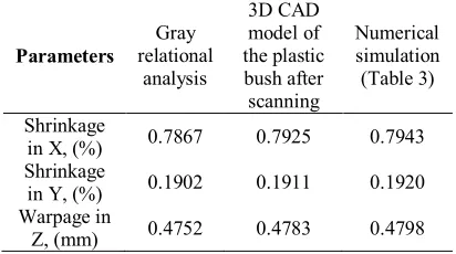
- Based on ANOVA Table, Mdie parameter with 45.75 and IR with 0.05 percent has the most and the least effect on the test conditions. - Table 12 includes the predicted values to determine the shrinkage in x and y directions, and also the warpage in z direction in grey relational analysis, and also the measurement of the 3D model of the plastic bush.
48
results. The values of shrinkage in x and y directions, and the values of warpage in z direction decreased about 0.95%, 0.93%, and 0.95% after the optimization process with grey relational analysis in comparison to the values presented in table 3. Also, the difference between the values predicted by grey relational analysis and the real manufactured plastic part is considerably low.
Table 12. Comparing of shrinkage and warpage values in three direction.
Parameters
Gray relational
analysis
3D CAD model of the plastic bush after scanning
Numerical simulation (Table 3)
Shrinkage
in X, (%) 0.7867 0.7925 0.7943
Shrinkage
in Y, (%) 0.1902 0.1911 0.1920
Warpage in
Z, (mm) 0.4752 0.4783 0.4798
16. Conclusions
In this paper, grey relational analysis was used to optimize two parameters, warpage and shrinkage, in manufacturing tractor plastic bush. The plastic used in manufacturing the bush is Derlin 500. The input parameters of the process are melt temperature, mold temperature, injection rate, injection pressure, and packing pressure. After designing the experiments with Taguchi method, the injection process was simulated in Mold Flow software based on these experiments. Then, with the help of grey relational analysis, and analysis of variance the optimum values for the input of the experiments were chosen and after that, the values of the plastic bush dimensional changes were predicted based on the confirmation test. At the end, by determining the optimal values the plastic bush was manufactured, and its 3D point cloud model was generated by a scanner and its dimensional properties were studied. Based on ANOVA Table, the two parameters of mold temperature and injection rate, with 47.75% and 0.05% respectively, have the most and the least effect on the experiment conditions.
The comparison of the results show that by using grey relational analysis the values of shrinkage in the x and y directions, and the value of warpage in the z direction decreased 0.95%, 0.93%,and 0.95% respectively. On the other hand, the difference between the values predicted by grey relational analysis and measuring and those of its 3D CAD model is very low.
Acknowledgement
This research project has been carried out with technical support of the Orumieh Tractor Manufacturing (O.T.M.Co).
References
[1] M. C. Huang and C. C. Tai, “The Effective Factors in the Warpage Problem of an Injection-Molded Part with a Thin Shell Feature”, J. Mater. Process Technol., Vol. 110, No. 1, pp. 1-9, (2001).
[2] S. J. Liao, D. Y. Chang, H. J. Chen, L. S. Tsou, J. R. Ho, H. T. Yau, W. H. Hsieh, James, T. Wang and Y. C. Su, “Optimal Process Conditions of Shrinkage and Warpage of Thin-Wall Parts”, Polymer Eng. Sci., Vol. 44, No. 5, pp. 917-928, (2004).
[3] Y. K. Shen, H. W. Chien and Y. Lin, “Optimization of the Micro-Injection Molding Process Using Grey Relational Analysis and Mold Flow Analysis”, J. Reinforced Plastic Composite, Vol. 23, No. 17, pp. 1799-1814, (2004).
[4] D. Kondayya, A. G. Krishna, “An Integrated Evolutionary Approach for Modeling and Optimization of CNC End Milling Process”, Int. J. Comp. Integrat. Manufact., Vol. 25, No. 25, pp. 1069-1084, (2012).
[5] S. H. Tang, Y. J. Tan, S. M. Sapuan, S. Sulaiman, N. Ismail and R. Samin, “The Use of Taguchi Method in the Design of Plastic Injection Mold For Reducing Warpage”, J. Mater. Process Technol., Vol. 182, No. (1-3), pp. 418-426, (2007). [6] H. Oktem, T. Erzurumlu and I. Uzman,
49 Technique in Determining Plastic
Injection Molding Process Parameters For a Thin-Shell Part”, Mater. Des.,Vol. 28,
No. 4,
pp. 1271-1278, (2007). [7] M. Altan, “Reducing Shrinkage inInjection Moldings via the Taguchi, ANOVA and Neural Network Methods”,
Mater. Des., Vol. 31, No. 1, pp. 599-604, (2010).
[8] G. Rajyalakshmi and P.V. Ramaiah, “Multiple Process Parameter Optimization of Wire Electrical Discharge Machining on Inconel 825 Using Taguchi Grey Relational Analysis”, Int. J. Adv. Manufact. Technol.,Vol. 69, No. 5, pp. 1249-1262, (2013).
[9] R. Ramanujam, N. Muthukrishnan and R. Raju, “Optimization of Cutting Parameters for Turning Al-SiC (10p) MMC Using ANOVA and Grey Relational Analysis”, Int. J. Prec. Eng. Manufact., Vol. 12, No. 4, pp. 651-656, (2011).
[10] N. Beri, A. Kumar, S. Maheshwari and C. Sharma, “Optimization of Electrical Discharge Machining Process with Cu-W Powder Metallurgy Electrode Using Grey Relation Theory”, Int. J. Mach. Mater., Vol. 9, No. (1-2), pp. 103-115, (2011). [11] K. Palanikumara, B. Lathab, V. S.
Senthilkumarc and J. Paulo, “Analysis on Drilling of Glass Fiber–Reinforced Polymer (GFRP) Composites Using Grey Relational Analysis”, Mater. Manufact. Process, Vol. 27, No. 3, pp. 297-305, (2012). ‘
[12] A. Sharma and V. Yadava, “Optimization of Cut Quality Characteristics during Nd: YAG Laser Straight Cutting of Ni-Based Super alloy Thin Sheet Using Grey Relational Analysis with Entropy Measurement”,
Mater. Manufact. Process, Vol. 26, No. 2, pp. 1522-1529, (2011).
[13] U. Caudas and A. Hascalik, “Use of the Grey Relational Analysis to Determine Optimum Laser Cutting Parameters with Multi-Performance Characteristics”,
Optics and laser Technol., Vol. 40, No. 7, pp. 987-994, (2008).
[14] B. Acherjee, A. S. Kuar, S. Mitra and D. Misra, “Application of Grey-Based Taguchi Method for Simultaneous Optimization of Multiple Quality Characteristics in Laser Transmission Welding Process of Thermoplastics”, Int. J. Adv. Manufact. Technol., Vol. 56, No. 9, pp. 995-1006, (2011).
[15] B. M. Gopalsamy, B. Mondal and S. Ghosh, “Optimization of Machining Parameters for Hard Machining: Grey Relational Theory Approach and ANOVA”, Int. J. Adv. Manufact. Technol., Vol. 45, No. 1, pp. 1068-1086, (2009).
[16] C. Y. Ho and Z. C. Lin, “Analysis and Application of Grey Relation and ANOVA in Chemical–Mechanical Polishing Process Parameters”, Int. J. Adv. Manufact. Technol.,Vol. 21, No. 1, pp. 10-14, (2003).
[17] S. Khalilpourazary, P. M. Kashtiban and N. Payam, “Optimization of Turning Operation of St37 Steel Using Grey Relational Analysis”, J. Comput. Appl. Res. Mech. Eng., Vol. 3, No. 2, pp. 135-144, (2014).
[18] M. Norhamidi, M. Nor, N. Hafiez, S. Ahmad, M. H. I. Ibrahim and M. R. Harun, “Multiple Performance Optimization for the Best Injection Molding Process of Ti-6Al-4V Green Compact”, Appl. Mech. Mater., Vol. 44, No. 1, pp. 2707-2711, (2011).
[19] S. Datta, A. Bandyopadhyay and P. K. Pal, “Grey-based Taguchi Method for Optimization of Bead Geometry in Submerged Arc Bead-on-Plate Welding”,
Int. J. Adv. Manufact. Technol., Vol. 39, No. 11, pp. 1136-1143, (2008).