An Algorithm for Plant Disease Visual Symptom Detection in Digital Images Based on Superpixels

Vol.9 (2019) No. 1

ISSN: 2088-5334

An Algorithm for Plant Disease Visual Symptom Detection in Digital

Images Based on Superpixels

Itamar F. Salazar-Reque

, Samuel Gustavo Huamán

, Guillermo Kemper

, Joel Telles

, Daniel Diaz

INICTEL-UNI, National University of Engineering, San Luis 1771, San Borja, 15021, Peru E-mail: *[email protected]

Abstract— Quantifying diseased areas in plant leaves is an important procedure in agriculture, as it contributes to crop monitoring

and decision-making for crop protection. It is, however, a time-consuming and very subjective manual procedure whose automation is, therefore, highly expected. This work proposes a new method for the automatic segmentation of diseased leaf areas. The method used the Simple Linear Iterative Clustering (SLIC) algorithm to group similar-color pixels together into regions called superpixels. The color features of superpixel clusters were used to train artificial neural networks (ANNs) for the classification of superpixels as healthy or not healthy. These network parameters were heuristically tuned by choosing the network with the best classification performance to obtain the automatic segmentation of the diseased areas. The performance of the classifier was measured by comparing its automatic segmentations with those manually made from a database with public and private images divided into nine groups by visual symptom and plant. The mean error of the area obtained was always below 11%, and the average F-score was 0.67, which is higher than that found by the other two approaches reported in the literature (0.57 and 0.58) and used here for comparison.

Keywords— segmentation; superpixels; leaf diseases.

I. INTRODUCTION

Estimating the severity of leaf diseases reliably is an overriding activity to predict yield losses, to monitor and forecast epidemics, to evaluate the resistance of plants to diseases, etc. However, not only is this procedure time-consuming, it requires qualified personnel [1]. Automatic segmentation of diseased leaf areas using image-processing techniques could provide solutions to such problems, though it reports its own extrinsic and intrinsic challenges. Extrinsic issues are those related to image acquisition artifacts such as changes in illumination and specular reflections, among others. Intrinsic issues, on the other hand, refer to processing problems such as ambiguous disease boundaries, multiple disease visual symptoms, and leaf isolation in a complex background [2]. Table I briefly summarizes these problems.

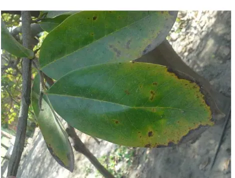
Figure 1 shows a Cherimoya leaf. In it, some extrinsic issues become evident: specular reflection and changes in illumination due to the position of the sun now of taking the picture. Intrinsic issues are also visible: Interest leaf isolation will not be an easy task, as the background is complex and composed of similar leaves, stems and soil; there is more than one visual symptom, and the yellow area boundaries are diffuse and difficult to determine, in contrast to the dark areas with more defined edges.

Fig. 1 Leaf sample image of a Peruvian native tree called Cherimoya, in which extrinsic and intrinsic problems are seen.

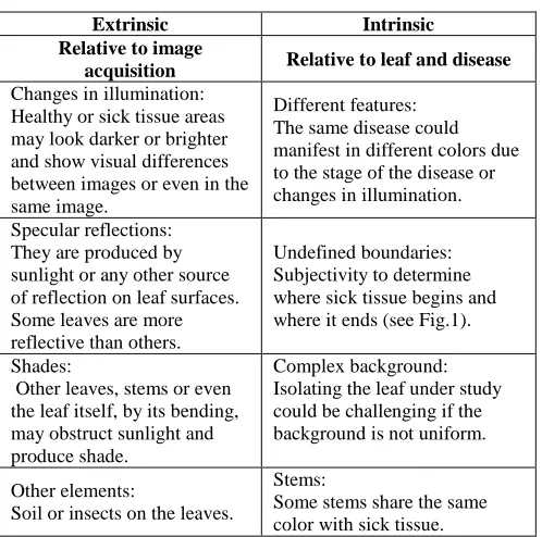
TABLE I

CHALLENGES IN AUTOMATIC SEGMENTATION OF DISEASED AREAS

Extrinsic Intrinsic

Relative to image

acquisition Relative to leaf and disease

Changes in illumination: Healthy or sick tissue areas may look darker or brighter and show visual differences between images or even in the same image.

Different features: The same disease could manifest in different colors due to the stage of the disease or changes in illumination. Specular reflections:

They are produced by sunlight or any other source of reflection on leaf surfaces. Some leaves are more reflective than others.

Undefined boundaries: Subjectivity to determine where sick tissue begins and where it ends (see Fig.1). Shades:

Other leaves, stems or even the leaf itself, by its bending, may obstruct sunlight and produce shade.

Complex background: Isolating the leaf under study could be challenging if the background is not uniform.

Other elements:

Soil or insects on the leaves.

Stems:

Some stems share the same color with sick tissue.

by Corythucha ciliata. In [4], Kruse et al. compared four methods to classify pixels of clover leave exposed to ground-level ozone; they reported the LDA (Linear Discriminant Analysis) classifier as the best of those evaluated. In [5], Pydipati et al. quantified diseased tissues in grapefruit leaves (Duncan variety) using texture metrics on the HSI color transform under laboratory conditions. In [6], Zhou et al. used a 2D color histogram to train a Support Vector Machine (SVM) classifier and determine if the tissue is damaged or not. In [7], Phadikar et al. proposed a Fermi energy-based method for the automatic segmentation of diseased areas in rice leaves. Using images of Oil Palm trees’ crown taken from a drone, Makky et al. [8] used ratios between color channels to find relationships with chlorophyll content which could be used to determine whether the evaluated leaf area is ill or not.

Not many research studies have tried to solve the automatic segmentation problem covering more than one disease in different plants. In [9], Camargo & Smith developed a method based on the analysis of the channel histograms from their color model (I3a, I3b, H) overall image. This analysis was used to perform adequate thresholding and generate masks that were then combined based on the maximum intensity values in each of the histograms. In [10], Barbedo developed a method for diseased area segmentation that uses two relationships obtained through pixel-level operations between RGB color channels to generate binary masks. Then, Boolean operations are applied to such binary masks to obtain the result.

However, these studies report problems when evaluating diffuse diseased areas, probably because assessing features pixel by pixel or globally is not as suitable as doing it taking into account neighboring pixels instead. Evaluating diffuse areas using algorithms that take into account only pixel-level data would lead to losing information, as the intensity distribution of neighboring pixels would not be considered,

which would result in false positives. On the other hand, doing only a global analysis would cause to lose local positional features.

In this work, superpixels have been used as a mechanism to preserve neighborhood features, grouping pixels together by color and spatial proximity. Later, a classifier (neural network) was trained using the superpixel features, generating binary masks that were then checked against the labeled reference images (ground truth). Reference image labeling is a determining and time-consuming procedure for the correct evaluation of classifiers and comparison with other approaches.

Although the Plant Village project [11] tried to offer a free plant image database (it was discontinued due to operating costs), there were no ground-truth images to be used as a reference. This is even more critical when we talk about more recent techniques such as deep learning, which requires not only computationally expensive training. However, a large number of training images and therefore manually labeled images.

This work is divided as follows. Section II introduces the set of images used, the superpixel generation procedure based on color and position, the parameters followed for artificial neural network design, and the quantitative validation procedure. Section III reports the results obtained when quantitatively comparing the proposed method with other methods. In Section IV, the results are discussed. Finally, in Section V, the conclusions are presented.

II. MATERIAL AND METHOD

The proposed methodology used a multilayer perceptron neural network to classify superpixels as healthy or not. The classifier was built using color characteristics taken from training superpixels (Figure 2); these characteristics were color transformations from the original image. In this section, we will describe the image database used and the conditions in which pictures were taken. Also, we will detail the proposed methodology’s most important blocks for image processing

A. Image database

Two hundred seventy-nine images of leaves were used, as divided into nine different groups by plant and disease. Table II provides a list of these groups, as well as a brief description of the visual manifestation of the disease and the number of samples per group.

Fig. 2 Flowchart of the proposed method.

The rest of the images were acquired from the Plant Village website. They belong to apple or grape leaves with visual disease symptoms in a uniform background; uniformity was obtained by placing a gray or black paper under the leaf of interest. Images have an approximate resolution of 600 x 800 pixels and 24-bit color depth and were taken under natural light conditions with a Sony DSC-Rx100/B 20.2 MP digital camera. For more information, see [11].

All of the images have 24-bits color depth (true color RGB) with primary components IR(x,y) , IG(x,y) and

) , (x y IB .

B. Background extraction

We specified that complex background consists of stems, other leaves, soil, among others (as shown in Figure 1) as this is a challenging task, which is still under study [12], some approaches use images acquired under controlled conditions [13]. The images used for this study have either a uniform or a complex background that must be removed before any procedure for diseased tissue segmentation.

Thus, complex backgrounds (Groups n = 4, 6, 7, 8 and 9 – Table I) were manually removed using free selection tool (Lasso tool) from GIMP 2.8 software, while uniform backgrounds (Groups n = 1, 2, 3 and 5 – Table I) were automatically removed by thresholding one of the channels of the image transformed into the hue (H), saturation (S) and value(V) color model, with components IH(x,y), IS(x,y)

and IV(x,y), or to the luminance (Y), blue chrominance

(Cb) and red chrominance (Cr) color model, with components IY(x,y), ICb(x,y) and ICr(x,y).

For automatic background extraction, we have used masks obtained by thresholding, which varies depending on the group the image belongs (see Table II). Such masks are generated as follows:

Group n = 1

 

 _{< <}

=

otherwise ,

0

51 . 0 ) , ( 2 . 0 , 1 ) , (

1

y x I y

x

b H (1)

Group n = 2

 

 _<

=

otherwise ,

0

48 . 0 ) , ( , 1 ) , ( 2

y x I y

x

b Cb (2)

Group n = 3

 

 _{< <}

=

otherwise ,

0

1 ) , ( 11 . 0 , 1 ) , (

3

y x I y

x

b S (3)

Group n = 5

 

 _<

=

otherwise ,

0

51 . 0 ) , ( , 1 ) , ( 5

y x I y

x

b Y (4)

Thus, a region of interest segmentation (only leaves) can be computed as:

) , ( ). , ( ) , (

'

y x b y x I y x

IR = R n (5)

) , ( ). , ( ) , (

' _{x y I x y b x y}

I_G = _{G n} (6)

) , ( ). , ( ) , (

' _{x y I x y b x y}

I_B = _{B n} (7)

where n specifies the group the image analyzed belongs.

C. Training and test samples

Sixty-eight representative images (25% of total), as classified into the nine different groups (each one with its corresponding binary mask), were chosen as training samples (see Figure 3).

Images with diseased areas in different parts of the leaf (apex, veins, center) were selected so that a good generalization is guaranteed when training our classifier. The remaining images became test samples used to verify the proper operation of the classifier.

D. Binary masks

Binary masks were made from the images of isolated leaves (Figure 3). Binary masks show diseased areas in white and the rest in black. They were also divided into training and test groups; the first is used to generate data for our neural network training, while the latter is used to quantify our method’s results and compare them with the approaches of Camargo [9] and Barbedo[10].

E. Superpixel generation

TABLEII SET OF IMAGES USED

Group n Plant and

disease Visual description Samples

1 Apple, scab Black or dark gray lesions on the leaf surface.

30

2 Apple, black rot

Circular light lesions with reddish or purplish margins.

30

3 Apple, cedar apple rust

Small bright yellow spots that gradually enlarge and change color to orange. They may show brighter concentric rings.

30

4 Avocado necrosis and infection

Necrosis: Dark margins. Infection: Yellow spots.

30

5 Grape, black rot

Circular black or brown lesion.

30 6 Mango,

necrosis

Brown spots with dark margins.

30 7 Potato,

Alternaria

White, black, brown and yellow spots.

39 8 Peach,

bacterial spot

Brown or black spots with a yellow halo.

30 9 Quinoa,

mildew Yellow spots.

30 Total 279

There are numerous techniques to generate superpixels. A review of such techniques is presented in [14]. For superpixel generation, we have used the approach presented in [15], which adapted the k-means grouping method to obtain the SLIC algorithm in which superpixels are produced from the groups obtained by proximity, as measured with a non-obvious distance D(x,y) from the 5-dimensional space generated by the CIELAB color model (with components

) , ( ' y x

IL , ( , )

'

y x

I_a and I_b'(x,y)) and from the position of the pixels in the image plane (x,y).

SLIC takes as input the quantity K of superpixels that is desired and follows the next procedure:

Step 1: The approximate step M between each group center is calculated as:

K N

M = (8)

where N is the number of pixels of the evaluated image, and K is the number of superpixels required.

Step 2: K centers of clusters are located (x&_k,y&_k); these centers are points in a 5-dimensional space, three of the dimensions being defined by CIELAB color space channels

(I_L'(x,y), _I'(_x,_y)

a and ( , )

' _{x y}

I_b ) and two by the position of pixels (x,y) in the image plane. The initial K centers (x&_k,y&_k) are separated by a distance M and are laid out in the space (x,y).

Step 3: Then, these K centers are relocated to pixels with smaller gradient values in a v × v window, in order to diminish the likelihood of centers being located in an edge or

noisy pixel. Gradients in a pixel located in x,y are calculated as follows: 2 ' ' 2 ' ' ' | ) 1 , ( ) 1 , ( | | ) , 1 ( ) , 1 ( | ) , ( − − + + − − + = y x I y x I y x I y x I y x F L L L L L (9) 2 ' ' 2 ' ' ' | ) 1 , ( ) 1 , ( | | ) , 1 ( ) , 1 ( | ) , ( − − + + − − + = y x I y x I y x I y x I y x F a a a a a (10) 2 ' ' 2 ' ' ' | ) 1 , ( ) 1 , ( | | ) , 1 ( ) , 1 ( | ) , ( − − + + − − + = y x I y x I y x I y x I y x F b b b b b (11)

The symbol “||” is the euclidian norm and the square window has a side v = 3. The new centers are defined as (x)_k,y)_k).

Step 4: Subsequently, the pixels in a 2M × 2M window at each K center is assigned to the nearest center measured at a distance D(x,y). Distance D(x,y) is not the Euclidean distance. Such distance considers the size of the superpixels to be generated and it is calculated as follows:

2 2 2 2_{( , )} ( , ) ) , ( m M y x ds y x dc y x

D_{k k} k _

      + = (12)

Where dc_kand ds_kbeing the Euclidean distance in colour

space (LAB) and spatial coordinates respectively.

(

)

(

)

(

)

2 ' ' 2 ' ' 2 ) , ( ) , ( ) , ( ) , ( ) , ( ) , ( ) , ( k k b b k k a a k k L L k y x I y x I y x I y x I y x I y x I y x dc ) ) ) ) ) ) − + − + − = (13)

(

) (

)

2 ) ,

( k k

k x y x x y y

ds = −) + −) (14)

Parameter m allows us to weigh the importance between

the similarity of color ( dc_k) and the spatial proximity (ds_k).

After this, K centers positions are recalculated as the average pixel position that belongs to the same group. Then, 2M × 2M square windows centered at the new superpixels centers are defined again, and the procedure is repeated ten times forcing connectivity in every iteration. This procedure results in K superpixels whose final centers are defined as ( x_0,k,y_0,k ) for k = 0,1,…, K-1. Figure 4 shows the

superpixels’ boundaries for iteration 1, 5 and 10. Note how they increase their regularity in every iteration.

We define pixels primary components which belong to

superpixel k from isolated image t as ( j,k, j,k) t

k x y

Lr ,

) , ( j,k j,k t

k x y

Lg and ( j,k, j,k) t

k x y

Lb . Here, (x_j,k,y_j,k) are the pixel coordinates which make up superpixel k. Then j has values j = 0,1,…, Pk – 1, where Pk is the number of pixels which determine superpixel k.

F. Training superpixels

Training superpixels were taken from pixel positions as randomly chosen from every representative image. Using ground-truth images, pixels were taken so that they belong to healthy and diseased areas equally. The location of each pixel corresponds to an image superpixel, our training data will be then obtained from these superpixels.

Fig. 4 Superpixels’ boundaries for iteration 1,5 and 10 in quinoa leaf.

G. Feature extraction

All the nine features correspond to the average values of the superpixel in every channel of the RGB color model and to the color transformations of these average values to the

HSV and YCbCr models. The result will be a vector Xt_kof nine elements per superpixel defined as:

] , , , , , , , ,

[ tk

t k t k t k t k t k t k t k t k t

k = R G B H S V Y Cb Cr

X (15)

where k is the superpixel number of image t. The following equations determine the elements of the vector:



j k j k j t k t k t

k Lr x y

P R (16)



j k j k j t k t k t

k Lg x y

P G (17)



j k j k j t k t k t

k Lb x y

P B (18)                   ₋       ₋ +       ₋       ₋ +       ₋ = − t k t k t k t k t k t k t k t k t k t k t k B G B R G R B R G R

H 1 ₂

5 . 0

cos (19)

      + + − = t k t k t k t k t k t k t

k R G B

B G R

S 1 3 min , , (20)

      = t k t k t k t

k R G B

V max , , (21)

t k t k t k t

k R G B

Y =0.063+0.257 +0.504 +0.098 (22)

t k t k t k t

k R G B

Cb =0.502−0.148 −0.291 +0.439 (23)

t k t k t k t

k R G B

Cr =0.502+0.439 −0.368 −0.071 (24)

A summary of the procedure used to obtain training features is shown in figure 5.

H. Classifier

Inspired by the mechanisms of communication between biological neurons, artificial neural networks (ANNs) consist of layers in which various artificial neurons are found. The neurons between one layer and the other are connected by links that simulate the synapse of their biological equals and whose intensity is governed by weights or parameters (W). These computing systems are usually used as classifiers. The first layer contains the input data, while the class corresponding to the input data is obtained from the last layer; between both, there are hidden layers whose parameters adapt to extract relevant information from the input data and perform the classification task through linear and non-linear transformations.

Figure 6 shows the artificial neural network architecture

used in this work. The input vector Xt_k propagates through the network, where weights W determine each neuron’s

contribution to the other neurons in the posterior layer. Each neuron is activated based on the activation function f. Training is an iterative procedure whose objective is to find the weights W that decrease the error, which is the

difference of the target Tkt and the output t k

s of the artificial neural network.

Thus, ANNs are non-linear modeling tools seeking relationships between previously known inputs and outputs for supervised training. This training process consisted in changing the weights of the connections between neurons according to pre-established rules in the training algorithm and reducing the error of the ANN output compared to the target associated with the input data.

In this case, superpixels were classified as healthy or not healthy based on their color features t

k

X , as specified in section G, which were used as input data to the neural

network. The corresponding targets T_kt were taken from the manually-created binary masks.

In this ANN, a single-hidden-layer topology has been established, in which the number of neurons has been found using the relationship proposed in [16].

1 2 + ≤ Q

r (25)

where Q is the number of inputs to the neural network, and r is the number of neurons in the hidden layer (in this case we have considered r = 19). Likewise, the output of each of the neurons in the hidden layer (pj) is determined by the propagation rule and the activation function of the neurons shown in the following equations:



=

+ = 9

1

1 1

, ,

i

j i j t k,i t

j

k X w

net θ (26)

1 1

2 )

(

,

2 ,

1

, −

+ = =

− t

j k

net t

j k t

j k

e net

f

p (27)

where X_k,it , represents the input i

,

: case In this

( Xk,t₁=Rtk 2 ,

t k t

k, G

X = Xk,t₃=Btk, 4 ,

t k t

k, H

X =

Fig. 6 Architecture of the artificial neural network used in this work.

, 5

t k t

k, S

X = X_k,t₆=Vtk, ₇ ,

t k t

k, Y

X = Xt_k,8=Cbtk and

); 9

t k t

k, Cr

X = w1_j,i , represents the weight that links the

hidden neuron j with the input neuron i; θ1_j, represents the

trend coefficient (bias) in neuron j of the first layer; t j k

net _, ,

is the value as calculated according to the propagation rule for neuron j, which will be evaluated in the activation function f1. The sigmoid hyperbolic tangent of the input defines the activation function f1 t

j k

net _, . Then, the output of

the neural network (s ) can be computed as: _kt





 

  

+ =

j

j t

j k j

j t

j k t

k f p w p w

s _{2 , 1}2 θ₁2 _{, 1}2 θ₁2 (28)

In this case, the activation function of the neuron in the

output layer (f2) is proportional;

2 ,i j

w , represents the weight

that connects the output neuron with the neuron of the

hidden layer j; θ12, represents the bias coefficient in the neuron of the output layer. The weight training algorithm is back-propagation, and it modifies the weights depending on

the errors found when comparing the output s with the t_k

target T . _kt

t k t k t

k s T

error = − (29)

A detailed explanation of the algorithm is found in [16].

I. Performance measures

positives (FP), which represent the number of healthy pixels incorrectly classified as diseased pixels; and false negatives (FN), which represent the number of diseased pixels incorrectly classified as healthy pixels. Another performance measure used was accuracy (ACC), whose calculation is obtained using the next equation.

FN FP TN TP

TN TP ACC

+ + +

+

= (30)

Additionally, the F-score and the Jaccard index (IJ) were calculated according to the following equations:

PRE TPR

PRE TPR score

F

+ × × =

− 2 (31)

FN FP TP

TP IJ

+ +

= (32)

where TPR is the true positive rate and is calculated as TPR = TP/(TP + FN); PRE is the precision, whose calculation is governed by PRE = TP/(TP + FP). The F-score and the Jaccard index are used because they correctly combine and penalize the similarities and differences between the obtained and desired results [17].

An important application of diseased area segmentation is the quantification of the infected area in the leaf under study. To study this application, the error has been calculated as the difference between the area obtained from the manually-segmented mask and the area of the mask calculated with the method under study (According to [9], [10] or the proposed method). The error is calculated as:

100 × −

=

manual manual calculated

area

A A A

e (33)

III.RESULTS AND DISCUSSION

The method proposed has been compared with the approaches in [9] and [10]. The comparison used the average TPR, ACC, F-score and IJ for each group. We have obtained values consistently greater than those of other approaches, thus demonstrating the robustness of our method. The TPR of the proposed method is in range of 0.42 to 0.90, which is higher than that of other approaches (Figure 7). The ACC is in the range of 0.55 to 0.98 and had similar variations that of the other two methods whose variations are in the range of 0.58 to 0.94 and 0.7 to 0.98 for [9] and [10], respectively (Figure 7).

The F-score is a complete measurement because it takes into account TPR and PRE values. The proposed method showed average values ranging from 0.56 to 0.80 (Figure 7). This range is narrower than the one of the methods proposed by [10] (0.33-0.83) and that [9] (0.38-0.73).

On the other hand, the IJ, which can be understood as the ratio between the intersection of the calculated mask and the manual mask and their combination, also presented less variable values in the proposed method (0.43-0.69) when

compared with [9], whose index ranged from 0.28 to 0.58, or [10], which ranged from 0.21 to 0.73 (Figure 7).

Fig. 7 Performance measurements of the methods proposed by Camargo [9], Barbedo [10] and our method.

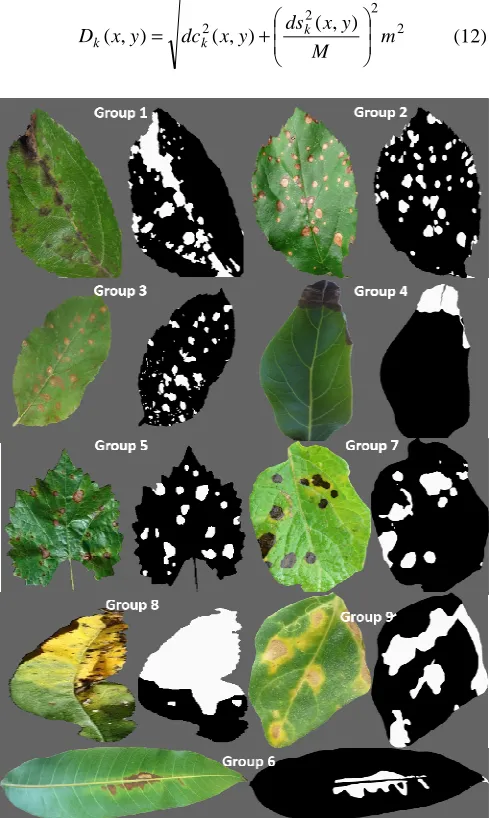
Figure 8 shows one image per group with its manually-created mask and the masks obtained when evaluating the picture with the proposed method and with the other two approaches. Images from groups 1, 8 and 9 show different diffuse zones. The masks obtained using the methods in [9] and [10] perform well only on the areas with strong visual disease symptoms, such as veins (group 1) or necrotic edges (group 8), but not on diffuse areas. In images of groups 2 and 5 (Figure 8), diseased areas are well contrasted with the background, which results in a similar performance by all three algorithms.

Evaluation of the area error allowed us to evaluate the use of the approaches in practical situations. Figure 9 presents quartiles and outliers in a boxplot diagram. In diagrams from Figure 9, we can see that the median error of the estimated diseased area using the proposed method is always below 10%, and in groups 1, 4, 5, 8 and 9, these values are lower than those of the others two methods. In groups 2, 3, 6 and 7, results are comparable to those of the other methods. However, the differences between the errors calculated with the other two methods are always under 6%. In the case of the image group 2, the median error evaluated using [9] is 2.9%, the one using [10] is 0.32%, and the one using our method is less than 0.5%; with the last two being quite accurate.

Fig. 9 Comparison of the area errors using the method proposed for Camargo [9], Barbedo [10] and our method.

In addition to the intrinsic challenges, there are also extrinsic difficulties such as the presence of soil, shadows or specular reflections, the latter being quite problematic because they are usually mistaken for disease, especially in images of plants whose leaves are very reflective, such as groups 4, 5 and 6, corresponding to leaves of avocado, grape, and mango, respectively. Therefore, it is best to take into consideration these conditions when taking the picture.

Another important source of error is veins, which in some cases are similar to the leaf, but in others make a great contrast with them; the color of diseased and healthy veins usually differs from those of leaves.

The issue was solved by using superpixels; part of the veins was grouped with the leaf surface and, when averaging color values, their influence was reduced

However, this does not usually occur with central veins, as they are more prominent. As said before, a benefit of using average color features on superpixels instead of common pixels is that the first incorporate leaf spatial color data and allow reducing some artifacts caused by pixels saturated by illumination or edge pixels. These conditions cause many false positives (FP) when evaluating pixel by pixel. Nonetheless, this benefit may be counteracted in the

presence of very small diseased areas, because average color features might cause the same effect as saturated pixels. It should be noted that, while spatial color features are important, texture features, as evaluated here according to work in [18], do not make significant contributions, but they increase the computational load and even generate false positives (FP). The reason is that the textures are generated on grayscale images, thus losing vital data for the correct discrimination of affected areas. It is, therefore, necessary to incorporate better color features that consider spatial data.

Image resolutions were slightly different with 600x800 pixels for groups n = 1,2,3,5 and 800x900 pixels for the rest. Therefore, as we have set the number of superpixels (K) to 800, each superpixel has in average approximately 600 and 650 pixels respectively. This makes 50 pixels of difference, which, for a leave of 10 cm with 600x800 resolution, represents approximately 0.8 mm2 of the area which is a negligible size for the naked eye. However, further work should be done to find how superpixels size alters segmentation.

classifies new data based on labeled data (training data) according to similarity with its k-neighborhoods, Support Vector Machine (SVM) and a Naive Bayesian Classifier (NBC) reported in [19]. Results show that SVM and NBC classifiers surpass the KNN classifier and their results similar to those obtained with the artificial neural network; improvements are mainly due to the use of superpixels.

TABLEIII

F-SCORES RESULTS WITH DIFFERENT CLASSIFIERS

Group KNN(1) KNN(3) SVM NBC

1 0.518 0.525 0.541 0.475

2 0.728 0.689 0.765 0.784

3 0.575 0.547 0.627 0.587

4 0.738 0.760 0.735 0.803

5 0.708 0.716 0.754 0.688

6 0.557 0.532 0.576 0.485

7 0.623 0.627 0.670 0.631

8 0.647 0.605 0.719 0.745

9 0.559 0.561 0.549 0.591

IV.CONCLUSIONS

The proposed method for the segmentation and estimation of diseased areas in plant leaves reports consistent results and, in most of the studied cases, shows a performance higher than that of the methods used for comparison. This means that the method allows detecting diseased areas based on a wide arrange of visual symptoms in a short time as the computational cost is not high. Like the other methods, the presence of specular reflections, shadows, and soil at the moment of taking the picture pose some difficulties that need to be taken into consideration. However, our method preserves neighboring characteristics that allow us to perform a proper segmentation even in diffuse areas where the other approaches are imprecise.

ACKNOWLEDGMENTS

To the National Innovation Program for Competitiveness and Productivity (Innóvate Perú) for the funds allocated to the project (388-PNICP-PIAP-2014). To the National Institute of Agrarian Research, the International Potato Institute, the Agro-Industrial Innovation Center for the Productivity in Moquegua and the Agrarian University of La Molina for allowing the acquisition of images of their crops. To the National Institute of Research and Training in Telecommunications (INICTEL-UNI) for providing the necessary logistical support for the development of the work.

REFERENCES

[1] C. H. Bocka, G. H. Pooleb, P. E. Parkerc, T. R. Gottwald, "Plant Disease Severity Estimated Visually by Digital Photography and Image Analysis and by Hyperspectral Imaging," Critical Reviews in Plant Science, vol. 29, no. 2, pp. 59-107, 2010. doi: 10.1080/07352681003617285.

[2] J.G.A. Barbedo, “A Review on the Main Challenges in Automatic Plant Disease Identification Based on Visible Range Images,”

Biosystems Engineering, vol. 144, pp. 52–60, April 2016. doi: 10.1016/j.biosystemseng.2016.01.017.

[3] A. Clément, T. Verfaille, C. Lormel, B. Jaloux, “A New Colour Vision System to Quantify Automatically Foliar Discolouration Caused by Insect Pests Feeding on Leaf Cells,” Biosystems Engineering, vol. 133, no. 0, pp. 128–140, 2015, ISSN 1537-5110. doi: 10.1016/j.biosystemseng.2015.03.007.

[4] O. M. O. Kruse, J. M. Prats-Montalbán, U. G. Indahl, K. Kvaal, A. Ferrer, C. M. Futsaether, “Pixel Classification Methods for Identifying and Quantifying Leaf Surface Injury from Digital Images,” Computers and Electronics in Agriculture, vol. 108, pp.

155-165, 2014. ISSN 0168-1699,

http://dx.doi.org/10.1016/j.compag.2014.07.010.

[5] Pydipati, R., Burks T.F. and Lee, W.S., "Identification of Citrus Disease Using Color Texture Features and Discriminant Analysis," Computer and Electronics in Agriculture, pp.49-59, 2006.

[6] R. Zhou, S. I. Kaneko, F. Tanaka, M. Kayamori, M. Shimizu, "Disease Detection of Cercospora Leaf Spot in Sugar Beet by Robust Template Matching," Computers and Electronics in Agriculture, vol. 108, pp. 58-70, 2014.

[7] S. Phadikar, J. Sil, A. Kumar, "Rice Diseases Classification Using Feature Selection and Rule Generation Techniques,” Computer and Electronics in Agriculture, vol. 90, pp. 76-85, 2013. doi: 10.1016/j.compag.2012.11.001.

[8] Makky, M., Yanti, D., & Berd, I. (2018). Development of Aerial Online Intelligent Plant Monitoring System for Oil Palm (Elaeis guineensis Jacq.) Performance to External Stimuli. International Journal on Advanced Science, Engineering and Information Technology, 8(2), 579-587.

[9] A. Camargo, J.S. Smith, "An Image-processing Based Algorithm to Automatically Identify Plant Disease Visual Symptoms,” Biosystems Engineering, vol. 102, no. 1, pp. 9-21, January 2009. ISSN 1537-5110. doi: 10.1016/j.biosystemseng.2008.09.030.

[10] J.G.A Barbedo, “A New Automatic Method for Disease Symptom Segmentation in Digital Photographs of Plant Leaves,” European Journal of Plant Pathology, vol. 147, no 2, pp. 349–364, 2016. doi: 10.1007/s10658-016-1007-6.

[11] D. P Hughes, M. Salathe, "An Open Access Repository of Images on Plant Health to Enable the Development of Mobile Disease Diagnostics,” CoRR, vol. abs/1511.08060, 2015.

[12] A. Borji, M.-M. Cheng, H. Jiang, and J. Li, “Salient Object Detection: A Benchmark,” IEEE Trans. Image Process. vol. 24, no. 12, pp. 5706–5722, Dec. 2015.

[13] Dinah, C., Sam, H., Usman, A., Tineke, M., & Makky, M. (2015). Optical characteristics of oil palm fresh fruits bunch (FFB) under three spectrum regions influence for harvest decision. International Journal on Advanced Science, Engineering and Information Technology, 5(3), 255-263.

[14] D. Stutz, A. Hermans, B. Leibe, “Superpixels: An evaluation of the state-of-the-art”, Computer Vision and Image Understanding, Volume 166, 2018, Pages 1-27, ISSN 1077-3142.

[15] R. Achanta, A. Shaji, K. Smith, A. Lucchi, P. Fua and S. Süsstrunk, "SLIC Superpixels Compared to State-of-the-Art Superpixel Methods," IEEE Transactions on Pattern Analysis and Machine Intelligence, vol. 34, no. 11, pp. 2274-2282, Nov. 2012. doi: 10.1109/TPAMI.2012.120.

[16] R. Hecht-Nielsen, "Theory of the Backpropagation Neural Network,” Proceedings of International Joint Conference on Neural Networks, vol. 1, pp. 593-605, 1989.

[17] V.Garcia, H. de Jesus Ochoa Dominguez, B. Mederos. “Analysis of Discrepancy Metrics Used in Medical Image Segmentation.” IEEE Latin America Transactions, 13(1), (2015) 235-240.

[18] C. Dharmagunawardhana, S. Mahmoodi, M. Bennett, M. Niranjan, “Gaussian Markov Random Field Based Improved Texture Descriptor for Image Segmentation,” Image and Vision Computing, vol. 32, issue 11, pp. 884-895, 2014. ISSN 0262-8856, http://dx.doi.org/10.1016/j.imavis.2014.07.002.