Arinola A. O. et al/LAUTECH Journal of Engineering and Technology 10(2) 2016: 30-37
30
MONTE CARLO SIMULATIONS FOR UNCERTAINTY QUANTIFICATION:
MATHEMATICAL FOUNDATION AND IMPLICATION OF UNDERLYING
ASSUMPTIONS
Akeem O. Arinkoola
1*, Kazeem K. Salam
1and Aladeitan M. Yetunde
21Petroleum Engineering Unit, Chemical Engineering Department, LadokeAkintola University of Technology,
Ogbomoso, Nigeria
2Chemical Engineering Department, University of Abuja, Nigeria
*Corresponding author
Abstract
Many problems in petroleum engineering involvesolving multivariable complex integrals andanalytic calculation is rarely possible in most practical cases. Numerical approximation appears to be practicable. However, majority of existing numerical solution of a D–dimensional integral with a relative accuracy (ϵ) requires a computation time proportional to ϵ-D. Hence, the use of Ordinary Monte Carlo simulation (OMCS) in uncertainty
quantification has gained tremendous attention. In reality, when historical data is available, variables are not independent and identically distributed (iid). The direct samplingof variable under this condition is not expected to be easy and use of OMCS can be erroneous. Methods based on Markov Chains will offer reasonable solution to this problem. This study evaluates simulation methodsfor quantifying uncertainty in reservoir forecast. The implications of underlying mathematics and assumptions that characterizes them were covered.The p5-p10–p50– p90-p95 uncertainty envelopes from different methods were presented using acase study from Niger Delta. The result is useful for identification and selection of effective tools in uncertainty quantification in the oil industry.
Keywords:
Numerical methods, Uncertainty, Markov chain, Monte Carlo
1.0 Introduction
Monte Carlo simulation is refers to simulation that utilizes random number and statistical analysis to compute results. It is very similar toany random experiments whose likely answer is not known. In this context, Monte Carlo simulation is considered a methodical way of doing “what-if analysis” (SamikRaychaudhuri, 2008).Petroleum engineering problems such as multi-phase and transport are usually integration problems. It is difficult to express a given reservoir performance perfectly as a closed function of a state and decision variables due to the associated uncertainties. Numerical solution of a multidimensional integral with reasonable accuracy requires a large computation time. Numerical Methods can handle more complex models but often characterize by repetition for each decision point. Analytical Methods can examine many decision points at once but limited to simple models (Gilks et al., 1996).
The preference for simulation methods is increasing despite availability of some asymptotic advantages of deterministic approaches to integration(R.Y. Rubinstein, 1981 andWilson andAdam, 1983). Deterministic methods are limited by high computing time. This is unacceptable to asset team in most cases because it affects developmental decisions. Simulation can handle very complex and realistic systems but has to be repeated for each decision
point. A more important fact is that simulation methods are generally straightforward for the investigator to implement. Itrelies on an understanding of a few principles of simulation and the structure of the problem at hand (John Geweke, 1996). Contrarily, deterministic methods typically require much larger problem-specific investments in numerical methods and assumptions in cases analytical solutions are sort.
Monte Carlo simulations are stochastic algorithms using the central limit theorem to compute multidimensional integrals (Liu and Oliver, 2003). Thus, with the central limit theorem, Monte Carlo simulationserror scales as ϵ-2, regardless of the dimensionality.
Every application of the Monte Carlo method can be reduced to a solution of a definite integral of form (Bernd and Alain, 2008).
= ( ) (1)
where domain Ω is a region in multiple-dimensional space and f(x) is the integrand. The integral I can be interpreted as the expected value of random variable f(X), where x is an independent random variable identically distributed (iid) in Ω. For practical application, the integral is usually of high dimensionality hence analytic calculation of an exact solution is not feasible. However, the approximate
Arinola A. O. et al/LAUTECH Journal of Engineering and Technology 10(2) 2016: 30-37
31
solution also requires a probability distribution, π from which set of samples, , … , in Ω is determined.The question this study set to address is that “What are the implications of different assumptions for the determination of point-estimate that reflect the actual structure of π?
Given a probability distribution, π, approximation of the integral ( )is the expected value (equation 2) using random sample x.
( ) = ( ) = ( ) ( ) (2)
Suppose are the upper and lower bounds of the integral, respectively, and that the region can be split into m intervals = < < . . . < <
= . Then the integral of a function (. ) is: ( )
= ( ) (3) In practice, may be infinite, in which case some cut-off point is required. In general, the cut-off are chosen so that the vast majority of the probability lies between such that:
( )
≈ 1 (4) The function can be approximated numerically using a polygon with an easy-to- compute area. There are literally many of such approximations, each with their own advantages and limitations.The rectangle rule approximates the area under the curve with a rectangle (equation 5). The rectangle rule provides exact solution only if the function was piece-wise flat.
ℎ( ) ≈ ℎ +2 ( − )(5)
Trapezoid rule improves the approximation by replacing the function at the midpoint with the average value of the function, and would be exact for any piece-wise linear function (including piece-wise flat functions).The trapezoid rule approximates the area under the curve with a trapezoid and is given by equation 6.
ℎ( ) ≈ℎ( ) + ℎ( )2 ( − )(6)
Simpson’s rule is based on using quadratic approximation to the underlying function. It is exact when the underlying function is piece-wise linear or quadratic. Simpson’s Rule approximation is given by equation 7.
ℎ( ) ≈ 6− ℎ( ) + 4ℎ +2 + ℎ( ) (7)
2.0 Ordinary Monte Carlo Simulations
Distinctions can be made between Monte Carlo Methods using graphical representation. For Ordinary Monte Carlo, the graphical model for naıve Bayes (Figure 1)withno edges between any of the nodeshas been used (Iain Murray, 2007). The features xd are dependent, but independent conditioned on the class variable c. Figure 1 is a directed graphical model for the joint distribution with class variable c and feature vector = . This simplest multivariate distribution assumes that all of their component variables x are independent.By implication, the independency of two measurable sets X1 and X2 (equation 8) implies any information about an event occurring in one set has no information about whether an event occurs in another set.
( ∩ ) = ( ) ( )(8)
One immediate implication of this assumption is that, the conditional probability of one given the other is the same as the unconditional probability of the random variable. This is impossible in practical sense.
( ⁄ ) = ( )(9)
Figure 1:Ordinary Monte Carlo Mathematically:
( )
= ( ) (10) The sum of this function divided by N will converge
to the expectation of the function as N becomes very large and the probability density (an estimate of < >and , its variance) in the large N limit can be written as
lim→ ( ) = 1
2 (11)
The estimate therefore becomes:
( ) ≈ ± (12)
3.0 Bayesian Simulations
Arinola A. O. et al/LAUTECH Journal of Engineering and Technology 10(2) 2016: 30-37
32
unknown quantities, and a prior distribution that describes ones beliefs about the unknown quantities independent of the data (Efendiev et al., 2006). Most commonly, the unknown quantities of interest are the parameters in a model, and the statistical model is the likelihood function ( ⁄ ). After collecting the data, one can update prior beliefs about and calculate the posterior distribution ( ⁄ ).Bayesian approach, expresses uncertainties in the model’s parameters θ in terms of probability. Parameter uncertainty is quantified first by introducing a prior probability distribution ( ), which represents the knowledge about θ before collecting any new data, and second, by updating this prior probability on θ to account for the new data collected (D).
This updating is performed using Bayes’ theorem, which can be expressed as:
= ( ⁄ ). ( ).( ⁄ ). ( ) (13)
Where ( ⁄ )is the posterior distribution of ; ( ⁄ ). ( ) is a normalizing constant required so that ( ⁄ ). = 1, and ( ⁄ )is the conditional probability for the measured data given the parameters. ( ⁄ )isoften referred to as the likelihood function.
Unlike ordinary Monte Carlo, the arrow directions in Figure 2 make a big difference compare with Figure 1.
Figure 2: Hidden causes
The xd are independent in the generative process. After observing y, knowledge about x forms a potentially complex joint distribution. Here, the direct sampling from is difficult. Methods based on Markov chains can offer a solution to this problem (Iain Murray, 2007).
Mathematically, ( , ) = ( )
= ( ) (14) Bayesian inference is carried out conditional on the observed data and does not rely on the assumption that a hypothetical infinite population of data exists. These differences give certain advantages to
Bayesian methods over ordinary Monte Carlo; such as that all inferences are exact and not approximated. 4.0 Case study
The use of uncertainty and risk analysis tools in the petroleum industry has increased since the first oil crisis. Uncertainty can emanate from numerous sources and directly impact the physical reservoir description (Vanegas et al., 2006). Monte Carlo simulation is usually combined to generate important probabilities that correspond to top-down figures with their corresponding values of parameters. The adoption of various methods is often based on discretions or practices with no or little attention been paid to the risks associated with decisions that came afterwards. The result from two Monte Carlo simulations for uncertainty quantification is presented.
This case study demonstrates the application of Ordinary and Markov-Chain Monte Carlo simulations in quantifying uncertainty of production forecast of a field in the Niger Delta.The study objective was to evaluate infill drilling potentials and quantify associated uncertainty. Evaluation and selection of infill opportunity was carried out by simulating reservoir incremental oil production and water breakthrough time from vertical and horizontal wells completed within the reservoir sub-regions the details on the field description is available online (Arinkoola et al., 2015).
4.1 Forecast performance model
The proxy model for the production forecast was approximated by the function:
y( , ) MMstb
= β + β SWI + β PERMX (15)
where SWI is the initial water saturation, PERMX is the horizontal permeability
ℎ = 2.488,
= 53.0332 = −17.2437.
4.2 Crystal ball - Ordinary Monte Carlo Simulation
The process starts with Equation15. One hundred thousand (100,000) uniformly distributed numbers between x to x , and y to y are randomly drawn using a Latin hypercube sampling techniquefrom a probability density function (Eqn. 16) obtained by dividing ( , ) by the total area under the curve.
( , )
= ( , )
( , ) (16)
A method of identifying ( , ) that makes more sense computationally is to utilize the cumulative distribution function. The pdf is transformed into a cumulative probability distribution.
Arinola A. O. et al/LAUTECH Journal of Engineering and Technology 10(2) 2016: 30
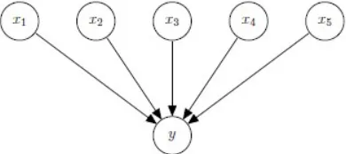
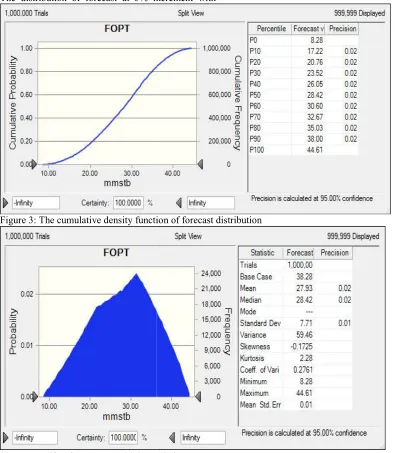
The results from the Crystal ball are presented as shown in Figure 3 and 4 as pdf and cdf respectively. The distribution of forecast at 5% increment with
Figure 3: The cumulative density function of forecast distribution
Figure 4: Pdf as forecast are with its statistics
Table 2: Forecast distribution and corresponding percentiles
Percentiles FOPT(MMSTB)
P5 14.67
P10 17.22
P50 28.42
P90 38.00
P95 40.03
4.3 WinBUGS - Bayesian Simulator
Arinola A. O. et al/LAUTECH Journal of Engineering and Technology 10(2) 2016: 30-37
33
The results from the Crystal ball are presented as shown in Figure 3 and 4 as pdf and cdf respectively. The distribution of forecast at 5% increment withcorresponding values of parameter is also presented in Table 2.
Figure 3: The cumulative density function of forecast distribution
Figure 4: Pdf as forecast are with its statistics
Table 2: Forecast distribution and corresponding percentiles
FOPT(MMSTB) PERMX SWI
14.67 0.61 0.66
17.22 0.64 0.67
28.42 0.93 0.77
38.00 1.22 0.87
40.03 1.25 0.89
WinBUGS is a windows version of the BUGS program for Bayesian analysis of complex statistical
37
nding values of parameter is also presented
Arinola A. O. et al/LAUTECH Journal of Engineering and Technology 10(2) 2016: 30
models using Markov Chain Monte Carlo (MCMC) techniques. WinBUGS allows models to be described using a slightly amended version of the BUGS language, or as Doodles (graphical representations of models) which can, if desired, be translated to a text based description.
4.3.1 Specifying model in the BUGS language The BUGS language allows a concise expression of the model, using the 'twiddles' symbol ~ to denote stochastic (probabilistic) relationships, and the left arrow ('<' sign followed by '-' sign) to denote deterministic (logical) relationships. The stochastic parameters β0, β1, β2 and τ in the proxy equation are given proper but minimally informative prior distributions, while the logical expression for sigma allows the standard deviation (of the random effects distribution) to be estimated. The model is specified as follows:
model {for (i in 1:N) { r[i] ~ dbin(p[i], n[i]) b[i] ~ dnorm(0, tau) logit(p[i]) <- beta0 + beta1*x1[i]+beta2*x2[i]+b[i]
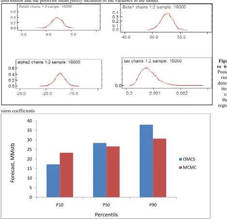
Figure 5 History plots showing two chains that are overlapped, an indication of convergence
Table 3 shows the posterior summaries of the parameters of the regression coefficients and the variance of the regression model. The posterior means and medians of the coefficients ofPERMX and
Arinola A. O. et al/LAUTECH Journal of Engineering and Technology 10(2) 2016: 30-37
34
hain Monte Carlo (MCMC) techniques. WinBUGS allows models to be described using a slightly amended version of the BUGS hical representations of models) which can, if desired, be translated to atext-Specifying model in the BUGS language The BUGS language allows a concise expression of the model, using the 'twiddles' symbol ~ to denote robabilistic) relationships, and the left ' sign) to denote deterministic (logical) relationships. The stochastic and τ in the proxy equation are given proper but minimally informative prior distributions, while the logical expression for sigma allows the standard deviation (of the random effects distribution) to be estimated. The model is specified
beta0 ~ dnorm(0, 1.0E beta1 ~ dnorm(0, 1.0E beta2 ~ dnorm(0, 1.0E tau ~ dgamma(0.001, 0.001)
sigma< }
To check the convergence of MCMC simulations while running the model, multiple chains with divergent starting points were run using derivative free adaptive rejection sampling algorithm.
Figure5 shows the trace plots for different parameters. The overlapping of the chains is an indication that reasonable convergence has been achieved after 11000 iterations. To obtain samples for posterior inference, Monte Carlo error was calculated for each parameter. A total of additional 10000 simulations were required to obtain Monte Carlo error less than 5% of the sample standard deviation for all parameters.
History plots showing two chains that are overlapped, an indication of convergence
shows the posterior summaries of the parameters of the regression coefficients and the variance of the regression model. The posterior means and medians of the coefficients ofPERMX and
SWI indicated that they are important variables. Moreover, we observe that the posterior means of β are slightly different from the ordinary least square estimates (2.152, 52.58, -17.31) T concluding that
37
} beta0 ~ dnorm(0, 1.0E-6) beta1 ~ dnorm(0, 1.0E-6) beta2 ~ dnorm(0, 1.0E-6) tau ~ dgamma(0.001, sigma<- 1 / sqrt(tau)
To check the convergence of MCMC simulations while running the model, multiple chains with divergent starting points were run using derivative-free adaptive rejection sampling algorithm.
shows the trace plots for different s. The overlapping of the chains is an indication that reasonable convergence has been achieved after 11000 iterations. To obtain samples for posterior inference, Monte Carlo error was calculated for each parameter. A total of additional were required to obtain Monte Carlo error less than 5% of the sample standard
Arinola A. O. et al/LAUTECH Journal of Engineering and Technology 10(2) 2016: 30
our prior was essentially a little bit informative
Table 3 Posterior summaries of the indicator parameters included in the Bayesian model node mean sd MC error
beta0 2.152 1.02 0.06495 beta1 52.58 1.041 0.06051 beta2 -17.31 0.993 0.05526
Figure 6 displays the posterior kernel density plots for model parameters βi. The posterior distributions of the coefficients are normal for all the variables. The posterior median of the
distribution and the posterior mean justify inclusion of the variables in th
ssion coefficients
Figure 7: Histogram showing comparison of forecast distribution using ordinary and Markov Chain Monte Carlo simulations.
0 5 10 15 20 25 30 35 40
P10
Fo
re
ca
st,
M
M
stb
Arinola A. O. et al/LAUTECH Journal of Engineering and Technology 10(2) 2016: 30-37
35
our prior was essentially a little bit informative implementing minor on the model parameters. ior summaries of the indicator parameters included in the Bayesian model
2.5% 10% 50% 90% 97.5%
0.06495 0.1555 0.8411 2.164 3.43 4.098 0.06051 50.47 51.21 52.61 53.89 54.51 0.05526 -19.36 -18.58 -17.29 -16.06 -15.4
displays the posterior kernel density plots for model parameters βi. The posterior distributions of the coefficients are normal for all the variables. The posterior median of the
distribution and the posterior mean justify inclusion of the variables in the model.
Histogram showing comparison of forecast distribution using ordinary and Markov Chain Monte Carlo
P50 P90
Percentils
OMCS MCMC
37
implementing minor on the model parameters.
start sample 12001 16000 12001 16000 12001 16000
displays the posterior kernel density plots for model parameters βi. The posterior distributions of the
Figu re 6: Poste rior densi
ties of the regre
Histogram showing comparison of forecast distribution using ordinary and Markov Chain Monte Carlo
Arinola A. O. et al/LAUTECH Journal of Engineering and Technology 10(2) 2016: 30-37
36
5.0 Conclusion
The OMCS indicated that the system under study was heterogeneous. This is evident from the extreme forecast distributions (P10 – P90) obtained. However, Bayesian analysis produced posterior estimates (P2.5%, P10%, P50% P97.5% and P90%) that are highly representative being fairly homogeneous typical of the system under study. The high uncertaintyassociated with the use of OMCS can largely be attributed to the assumption of parameter independency on the forecast. When parameters are not independent (iid) the application of Ordinary Monte Carlo analysis around a history match is not valid. A full Bayesian treatment is required.
6.0 Conflict of Interest
The authors declare that there is no conflict of interests regarding the publication of this paper. References
SamikRaychaudhuri (2008), Introduction to Monte Carlo Simulation, Proceedings of the 2008 Winter Simulation Conference, USA
Gilks, W.R., Richardson, S., Spiegelhalter, D.J. (eds.): Markov Chain Monte Carlo in Practice. Chapman & Hall, New York (1996)
John Geweke (1996), Monte Carlo Simulation and Numerical Integration, Handbook of Computational Economics, Volume I Elsevier Science publisher Liu, N., Oliver, D.S.: Evaluation of Monte Carlo methods for assessing uncertainty. SPE J. 8(2), 188– 195 (2003)
Wilson B. C., Adam G., “A Monte Carlo model for the absorption and flux distributions of light in tissue,” Med. Phys.. 10, (6 ), 824 –830 (1983). 0094-2405).
Bernd A. Berg1, Alain Billoire, Markov Chain Monte Carlo Simulations, Wiley Encyclopedia of Computer Science and Engineering, edited by Benjamin Wah, 2008 John Wiley & Sons, Inc.
R.Y. Rubinstein, Simulation and the Monte Carlo Method (John Wiley & Sons, New York, 1981) Iain Murray. Advances in Markov chain Monte Carlo methods. PhD thesis,Gatsby computational neuroscience unit, University College London, 2007 (page 14 - 20)
Efendiev, Y., Hou, T., Luo, W.: Preconditioning Markov chain Monte Carlo simulations using coarse-scale models. SIAM J. Sci. Comput. 28(2), 776–803 (2006)
VanegasJW, Cunha JC, Cunha LB (2006). “ Uncertainty Assessment of production Performance for a Heavy Oil Offshore Field by using the Experimental Design Technique”, paper 2006-125 presented at the Petroleum society’s 7th Canadian International Petroleum Conference, Calgary, Alberta, Canada, June 13-15, 2006.
ArinkoolaA O, Haruna M O, Ogbe D O (2015). Quantifying Uncertainty in Infill well Placement using Numerical Simulation and Experimental Design, J. Petrol Explor Prod Technol, ISSN 2190-0558, DOI 10.1007/s13202-015-0180-z