game theory notes

(1)

Lecture Notes for Ph.D. Game Theory

∗

Philip R. Neary

†

∗_{These notes attempt to fuse material from a course taught by Joel Sobel at UCSD with material} from Mas-Colell, Whinston, and Green (1995), Osborne and Rubinstein (1994), and Van Damme

(1996). They probably contain loads and loads of mistakes. Please let me know me if and when you find any. Updated: March 3, 2014

(2)

Introduction

Last term Chris introduced you to Decision Theory. He showed you a wide range of analytical techniques designed to help a decision maker choose amongst a set of alternatives in light of the consequences of each. He began with how to model a decision maker’s preferences, and then, given such preferences, how the decision maker ought behave in situations with risk, uncertainty, etc.

One key feature of last term was that in all the models, there was only ever one economic agent. But there are many situations of interest involving more than one agent. Game Theory is a formal framework for situations of this nature, as it provides tools to analyse how a decision maker ought behave when his payoff depends not only on his own actions, but also on the actions of others. It can be thought of, and is even sometimes referred to, as interactive decision theory, just as decision theory can be thought of as 1-player game theory.

Another way to say this is that Game Theory takes the underlying premise of Decision Theory - agents are rational (i.e., they pursue well-defined objectives) - and adds a strategic aspect whereby agents care not only about their own actions but also about the actions of others. This is the key feature of game theory and so I will emphasise it again: the payoff that an agent gets from making a particular decision may depend on the decisions of others. Thus, even in very simple settings with no outside risk, uncertainty, etc., a game can be difficult to analyse, since there is still something that the decision maker does not have control over: the behaviour of others.

While Game Theory began as a branch of applied mathematics, it has been hijacked as the formal language of choice by social scientists for describing strategic situations. Researchers proceed via the following steps:

1. Start with a strategic problem

2. Translate the problem into a game

3. Solve the game

4. Translate the solution back to the motivating problem

The first step involves finding an interesting research question. This is hard. The second step requires constructing a mathematical model that describes the situation. This is not easy and is something of an art. The third step is both philosophical and technical. First one must decide on what it means to be a solution, and then one must take the solution concept and apply it. The fourth step is easy, although people often exaggerate wildly.

• The first part of this course is essentially about step 3.

(4)

Like any academic discipline game theory can be divided along many different dimensions, but one extremely natural division is that of cooperative ‘vs’ non-cooperative game theory. A non-cooperative game is a game where players choose strategies independently.1 _{A cooperative game is one in which groups of players}

(re-ferred to as “coalitions”) may enforce cooperative behaviour. Hence the competition is between coalitions rather than between individuals. This course is exclusively about non-cooperative game theory.

Before getting to game theory, I will very briefly review “rational” decision making - in particular decision making under uncertainty.

2

Individual Decision Making

2.1

Choice Under Certainty

The take off point of individual decision making is a set of objects, thechoice set, from which the individual must choose. I will denote this byX. Typical elements of X will be denoted byw, x, y, andz. The elements of X are mutually exclusive and exhaustive. That is, for example, if you choosex then you cannot choosey. And there is no choice “not inX”.

The next component to specify is a preference relation over elements in X. This is the primitive of the individual. This preference relation is simply a binary relation on X that satisfies some fundamental properties called axioms. There are a host of properties that binary relations may satisfy, but we will only require a few. In addition to making intuitive sense, there are two technical properties that a collection of axioms should satisfy. Our set of primitive axioms should be:

(i) consistent, meaning that each axiom can be satisfied simultaneously.

(i) independent, meaning that none of the axioms are redundant, i.e., that no subset of the axioms implies the others.

Suppose we have a binary relation on the set X denoted by R. Formally this is a collection, R, of ordered pairs (x, y), with x, y ∈ X. In other words, R ⊆ X. If (x, y) ∈R, it is standard to write xRy. This can be read as “x is related to y”. If “x is not related toy”, so that (x, y)6∈R, it is conventional to write xRy. I now list some˜ properties that a binary relation may satisfy. A binary relationR on X is said to be:

• reflexive: if for all x∈X it holds that xRx

• irreflexive: if for all x∈X it holds thatxRx˜

(5)

• symmetric: ifxRy implies yRx

• antisymmetric: ifxRy and yRx imply y=x

• asymmetric: ifxRy implies yRx˜

• transitive: if for all x, y, z ∈X,xRy and yRz imply xRz

• negatively transitive: if xRz implies that, for all y ∈ X, either xRy or yRz or both.

for all x, y, z ∈X, xRy˜ and yRz˜ imply xRz˜

• complete ortotal: if for all x, y ∈X, eitherxRy oryRx or both

• acyclic: if x1Rx2, x2Rx3, . . . , xn−2Rxn−1, xn−1Rxn imply x1 6=xn.

A binary relation that is reflexive, symmetric, and transitive is called anequivalence relation. A binary relation that is reflexive, antisymmetric, and transitive is called a partial order. A partial order that is complete or total is called a total order or sometimes alinear order. A linear order where every nonempty set has a least element is called a well-order.

Once we have decided on our (minimal and consistent) collection of axioms from the list above, we will declare a binary relation that conforms to them as beingrational

since it captures how a decision maker ought behave, and declare that we now have a preference relation. We then analyse how the rational preference relation will affect decision making.

Given a preference relation, the goal is to prove a representation theorem. What we seek is to start with the preference relation and derive a real-valued function from the choice setX that is equivalent to the relation. In other words, the utility function should rank all pairs of objects from X in the same way as . This function is often called autility function. In other words we want to show that the axioms are sufficient for the utility function, meaning that when the axiom holds, you can find a utility function that ranks alternatives in the same way. And we also want to show that the axioms are necessary for the representation, meaning that if the representation holds, then the axioms must as well.

So, we have a set from which choices must be made, X, and we want to define a binary relation on pairs of objects from this set that is “rational”. What we take as our primitive binary relation, denoted by , one connoting “strict preference”. That is, we write xy if the decision maker strictly prefers x to y. If x is not preferred to y, writexy.

Ok, so now let’s get to the axioms that we will assume.

Definition 1.A binary relationonXis called apreference relationif it is asymmetric and negatively transitive, i.e.,

(6)

• negatively transitive: if x z implies that, for all y ∈ X, either x y or y z or both.

Here is the first result.

Proposition 1. If is a preference relation, then is irreflexive, transitive, and acyclic.

Some authors prefer to begin with an alternative binary relation that connotes weak preference interpreted as “at least as good as”. This is denoted by _%, where we write x_% y if y x. Naturally, this leads to the same conclusions. We can also define the

indifference relation, ∼, defined as x∼ y if xy and y x (or analogously as x _%y and y_%x).

In words, we say that “x is weakly preferred toy if yis not strictly preferred to x”, and “the decision maker is indifferent betweenxand yif neither is strictly preferred to the other”.

The following proposition relates our three binary relations ,_%, and ∼. Proposition 2. If is a preference relation, then

(a) For all x, y ∈X, exactly one of xy,y x, or x∼y holds.

(b) _% is complete and transitive

(c) ∼ is reflexive, symmetric, and transitive

(d) wx, x∼y, yz, together imply that wy and xz.

(e) x_%y if and only if xy or x∼y (f) x_%y and y_%ximply x∼y

We are now ready to introduce utility functions. The goal is to take the preference relation, , defined above, and to construct a numerical representation that ranks all pairs fromXin exactly the same way. Formally, we are looking for a functionu:X →_R

such that

xy if and only if u(x)> u(y) (1)

Our first representation theorem is stated for the case where the choice set X is finite.

Theorem 1 (Simple Representation Theorem). Suppose we have finite choice set X. A binary relationsucc onX is a preference relation if and only if there exists a function

(7)

You should be able to prove the “if” direction without too much bother. That is, assume there exists a function u and show that is a preference relation. The other direction is harder.

We would like to extend Theorem 1above to the case where the set X is arbitrary, in particular to allowing for it to belarge. There are two notions of large (infinite) of interest here. The first is to let X be countably infinite, and the second for it to be

uncountably infinite.

Theorem 1 can be shown to hold true when X is countably infinite, but not so when uncountable. The well-knownlexicographic preferences can be used to provide a counterexample. To extend the result to include uncountable choice sets, some addi-tion topological restricaddi-tions (relative to the relaaddi-tion ) on the set X are required. In particular, it is required thatX possess a -order-dense subset.2

The last thing I will say here is a quick comment onuniqueness. You will often hear that the representation constructed from the preference relation is unique. This is not really true. Actually the representation is unique up to a strictly increasing trans-formation. That is, if the representation constructed is denotedu, then for any strictly increasing g : _R → _R, the compostive function g ◦ u also represents the preference relation.

2.2

Choice Under Uncertainty

What we want to do in this section is to extend that of 2.1 to allow for the objects in the choice set X to represent uncertain prospects, commonly called lotteries. Fist of all we need a way to model uncertain prospects. There exists more than one way to do this, but the avenue we pursue is due toVon Neumann and Morgenstern (1944) and is conceptually the simplest. However, we pursue this direction as it carries over nicely to the study of games.

The fundamental component used here is that the uncertainty is objective. That is, the various different outcomes each have a given likelihood as specified by a fixed probability distribution. The uncertainty is imposed from the outside (by God perhaps). There is nothing the decision maker can do to affect the uncertainty.

Formally, consider a set ofoutcomes, given by Z, together with a set of probability distributions/measures defined on Z, given by P. In this framework, the preference relation will be defined over pairs of objects in P. That is, our choice set is P. Let’s look at a simple example.

Example 1. Suppose that there are only two outcomes, £0 and £100, so that Z :=

{£0,£100}. The set of distributions,P can then be parameterized by a single number, p, in the interval [0,1], where p is the likelihood of the outcome £100 (and so clearly

(8)

1−p is the likelihood of £0). That is, P :={p|p is the probability of£100}. Note: there is really only one sensible preference relation in this case.

Now let’s make this more general. First we need to consider what is the set of allowable distributions. WhenZ is finite, there are no issues - simply let P denote the set of all probability measures on Z. That is, P :=

p:Z →[0,1]| P

z∈Zp(z) = 1 .

However, as with decision making under certainty, a technical hitch arises when Z is infinite. Note however, that even when Z is finite (and provided it has two or more elements), the choice set P is infinite.

For now we will gloss over the axiom part of the analysis and move on to the utility representation. What I will say is that two of the axioms meant that the relation

is a preference relation in the sense of Definition 1. However, there are two other axioms that are required. These are typically called the independence axiom and the

Archimedean axiom. I suggest you look them up. So we assume four axioms:

Axiom 1 (Asymmetry).

Axiom 2 (Negative Transitivity).

Axiom 3 (Independence axiom).

Axiom 4 (Archimedean axiom).

Taken together, Axioms 1-4 yield the following representation theorem.

Theorem 2 (Expected Utility Representation Theorem). A binary relation on P

satisfies Axioms 1-4 if an only if there exists a function u:Z →_R such that

pq if and only if X

z∈Z

p(z)u(z)>X

z∈Z

q(z)u(z) (2)

Some things are worth mentioning. Theorem2above is also described as a “unique-ness result”, and as before this is slightly misleading. What this means is that the function u above is unique up to an affine transformation. That is, if u satisfies the conditions of the Theorem, then so does the functionv where for a positive real number a and any real number b, v(·) = au(·) +b.

There is sometimes confusion in the terminology. In particular be careful when reading Mas-Colell, Whinston, and Green (1995). They refer to the function u in (2) as the Bernoulli utility function. The weighted sum of the us is the von Neumann Morgernstern utility function. That is, the real-valued function defined on P. For a given lotteryp∈P, we write

U(p) :=X

z∈Z

(9)

3

Strategic Games

A strategic game is a model of interactive decision-making where each decision-maker chooses a strategy independently, and all players do so in ignorance of what the others are choosing (so that we can think of them as choosing simultaneously). Formally, it is a well-defined mathematical object comprised of three things. The first is theplayer set. This describes who is playing the game. Players can be people, firms, countries, animals, etc. The second are the strategies available to each player. Using the examples of players listed above these could be buy/sell, set a high/low price, attack/don’t attack, fight/flee. Finally, it specifies a utility/payoff function for each player, where the utility that a player gets depends on the actions that all the players take. Here is our first definition,

Definition 2. A strategic game, also called a normal-form game, is defined as a triple Γ =nN,{Si}n_i=1,{Ui}n_i=1

o

, where

• N ={1, . . . , n} is a finite set of players,

• {Si}n_i=1 is a collection of finite, nonempty strategy sets, one for each player,

• {Ui}n_i=1 is a collection of utility functions, one for each player, defined on S := Qn

j=1Sj.

IfSi is finite for each player i, then Γ is a finite game.

It is useful to comment on what information the players have. Do players know what their own strategies and payoffs are? Well, if they are going to be both purposeful and goal-orientated they must! Throughout this course we will assume something far stronger - that the structure of the game, the mathematical definition given in Definition

2, is “common knowledge”. This means that for a given game Γ: everybody knows Γ, everybody knows that everybody knows Γ, everybody knows that everybody knows that everybody knows Γ, and so on. We will look at common knowledge in more detail towards the end of the course.

What happens in a playing of the game is the following. At exactly the same time, all players choose a strategy from their available set. That is, player 1 chooses some s1 ∈S1, player 2 chooses somes2 ∈S2, etc. This generates astrategy profile oroutcome

s= (s1, . . . , sn)∈S, which describes what occurred. Given outcome s, each player gets

a utility. Player 1 getsU1(s), player 2 getsU2(s), etc. Note that these utility functions

are Bernoulli utility functions as defined at the end of Section2.2.

While Definition 2 is extremely general, let’s begin by looking at some simple ex-amples involving only 2 players. I will be very slow and deliberate in discussing the first example. For the later examples I will briefly describe some of their interesting features.

(10)

1

2

h t

H 1,−1 −1,1 T −1,1 1,−1

The story goes like this. There are two players, each of whom has a coin. Each player chooses a side of the coin, either Heads or Tails, and puts that side face up on the table with their hand covering the coin. Then, they simultaneously remove their hands to display what side of the coin they chose. If the two faces match then Player 1 keeps both coins; if they don’t match then Player 2 keeps both coins.

The matrix representation depicts one row for each strategy of player 1, and one column for each strategy of player 2.3 _{Each cell of the payoff matrix corresponds to}

a strategy profile. In each cell, the first number is Player 1’s payoff, and the second number is Player 2’s payoff from the corresponding profile.4

Ok, now let’s beat this to death. There are 2 players, each with the same set of available actions {heads, tails}, that, for reasons of clarity, I have labelled differently for each player.

• The player set is N ={1,2}

• S1 ={H, T}, and S2 ={h, t}.

• S =S1×S2 ={(H, h),(H, t),(T, h),(T, t)}.

• Payoffs from each strategy profile are as follows:

· U1 (H, h)

= 1; U2 (H, h)

=−1

· U1 (H, t)

=−1; U2 (H, t)

= 1

· U1 (T, h)

=−1;U2 (T, h)

= 1

· U1 (T, t)

= 1; U2 (T, t)

=−1

Now let’s look at some more 2-player examples.

Example 3 (Call Back). This is our first game of coordination.

1

2 Call Wait Call 0,0 2,2 Wait 2,2 0,0

3_{In any game with two players called ‘1’ and ‘2’, I adopt the convention of calling the row player} ‘player 1’.

(11)

There are two friends on the phone to each other when the line goes dead. They want to resume the conversation. Each player can attempt to call back, or wait for the other to call. If they both call then they receive busy signals, if they both wait then clearly they don’t talk. This game has two sensible predictions, both of which are unsurprisingly referred to as “coordinated outcomes”.

Question: How would things change if each player preferred for the other to call since phone calls aren’t free?

Example 4 (Dominant Strategy). This is a game with a so-called dominant strategy.

1

2 Left Right Up 10,1 2,0 Down 5,2 1,100

The interesting feature of this game is that no matter what player 2 does, player 1 should play ‘Up’. If player 2 does a little bit of thinking then he will realise that he is essentially faced with a simple decision problem, where he must choose between the two cells in the top row. Thus Player 2 should choose ‘Left’ even though she herself is ruling out any chance of her preferred payoff.

So, the fact that player 1 had a clearly optimal (“dominant”) strategy allowed us to make a reasonably clear prediction.

Example 5 (The Prisoner’s Dilemma). This is a game where both players have a dominant strategy.

1

2

Cooperate Defect Cooperate 4,4 0,5

Defect 5,0 1,1

This is one of the most famous games in all of game theory. It is interesting since both players have a dominant strategy (and provided that the stated payoffs accurately reflect how players feel about outcomes, taking a dominant strategy is clearly a sensible thing to do), and yet if both players choose their dominant strategy the result is inefficient. That is, the players would both be better off if they both chose ‘Cooperate’, but unfortunately, you can never rely on either to do this.

Example 6 (The Battle of the Sexes). This is another coordination game. It differs from that in Example3in that while the players want to coordinate, there is a tension since they want to coordinate on different things.

1

2

(12)

This is another extremely famous game. The story is that there is a couple, a woman (player 1) and a man (player 2), who want to meet up on a Friday evening. They always meet at one of two places, the Opera or the Football Match, and tonight is no different. The problem is that they did not decide on this week’s venue, and they cannot contact each other.5 So each must independently pick a venue. The tension occurs because while they each enjoyother’s company and hence want to meet, the woman prefers that they meet at the Opera while the man prefers they meet at the Match.

Example 7 (Matching Pennies Extended). The story is similar to that of Example 2

with one small difference. We now assume that Player 2 is a cheater. (Just assume that he has found some way of observing player 1’s coin before he must make his own move.) The most important thing to observe in the matrix below is that player 2 now has fourand no longer just two strategies.

1

2

hh ht th tt

H 1,−1 1,−1 −1,1 −1,1 T −1,1 1,−1 −1,1 1,−1

So why does player 2 have four and not just two strategies even though clearly all he is gonna do is that put the coin with either Heads facing up or with Tails facing up? And what the hell does, for example, ‘th’ mean?! The answer is subtle and is our first illustration of how general the notion of a strategy can be. Hopefully this will become very clear when we study extensive form games in Section 9, but for now think of it like this. While player 2 is moving after player 1, the strategic form representation cannot convey this and depicts players as moving simultaneously. So we should think of a strategy for player 2 as being a playbook that he leaves for someone else to carry out his wishes. Thus, for example, the strategyth means: “Playt if you observe player 1 playH, and play h if you observe player 1 play T”.

4

The Beginnings of Strategic Behaviour

So far we have just looked at some simple games and noted how strategy profiles translate to payoffs. We have not said anything about what players will do / should do. This section will touch on the surface of this, hinting at what players should not do, and in some games what they definitely should do.

But before we get to this, let’s take a quick detour on notation.

4.1

Notation

Players are acting independently, and so we will often analyse the situation from the perspective of only one player. A typical player will be referred to as i, j, or k. Note

(13)

that by analysing the strategic setting from the perspective of only one player, once we fix that player’s beliefs, the setting can be viewed as something similar to a decision problem.

Recall that each player i chooses a strategy si ∈Si. And when everybody chooses

a strategy, we get a strategy profile (s1, . . . , sn), and then can assign payoffs as we

did in the games above. When player i makes a strategic decision, he considers the strategies of the other players. Thus, from player i’s perspective, a typical strategy profile s = (s1, . . . , si, . . . sn) can be viewed as (si,s−i) where si is the strategy that i

chooses, ands−i = (s1, . . . , si−1, si+1, . . . , sn) is the (n−1)-dimensional vector connoting

the strategies that all players except playeri choose. Just ass∈S=Qn_j=1Sj, we have

that s−i ∈S−i = Q

j6=iSj.

4.2

Conjectures

How do players decide what strategies are good/bad? Well, as mentioned before, the core feature of game theory is that a strategy may be good/bad depending on how others behave. (An example would be deciding what side of the road to drive on. In the UK, it is a good idea to drive on the left hand side; in the US however, this is not so wise.) Thus a strategy needs to be evaluated relative to what the rest of the population is doing, and this evaluation needs to be done for every conceivable thing they rest of the population may do.

Thus, we will imagine each player compares the payoffs he would get from his various strategies assuming that the rest of the population’s behaviour is held fixed. But to do this we, the modeller, need to speculate about what players think their opponents will do. The way we will do this is to look at the players individually. Specifically, we will focus on a particular playeri, and suppose that playericonjectures that his opponents behave in a particular way. Using the notation we defined previously, a conjecture of player i is given by a particular s−i. So, with player i’s conjecture as s−i, and for any

two of player i’s strategies, s0_i and s00_i, we can now compare player i’s payoffs at the two strategy profiles (s0_i,s−i) and (s00i,s−i), since these two strategy profiles differ only

in playeri’s choice of strategy. We can then do this for all pairs of strategies of player i. To be thorough, we must then do this for all strategy profiles, and then repeat the entire procedure by doing it for each players. Clearly this is a huge operation, but fortunately there are some shortcuts available.

4.3

Dominance

Now let’s work through a few formal definitions. We will first focus on those strategies that it is reasonable to assume a rational player will take. These strategies are inherently “good”, and any reasonable model of strategic behaviour must advise agents to take them.

(14)

we have that

Ui(s∗i,s−i)> Ui(si,s−i), for all s−i ∈S−i

Thus, s∗_i is strictly dominant for player i if it is guaranteed to yield player i the highest payoff he can get for anything that his opponents do.

So if player i has a dominant strategy, it is a good bet that he will take it, since he cannot expect a higher payoff from taking anything else. In effect, the existence of a dominant strategy for a player reduces the potentially complex multi-player game to a very straightforward decision problem. From the standpoint of rational behaviour, a player must take a dominant strategy. Dominant strategies provide a very good guide to behaviour.

While dominant strategies are our first encounter with a sensible prescription of play, there are two problems with them,

• Other people’s decisions are not always irrelevant. (A coordination game is a clear example.)

• Even if a dominant strategy exists for all players, this sort of behaviour individual by individual could lead be collectively crazy (i.e. very inefficient) outcomes. A good example of this is the Prisoner’s Dilemma in Example 5.

The “opposite” to a strictly dominant strategy is astrictly dominated strategy. Just as a strictly dominant strategy was a “good” prescription of play, a strictly dominated strategy is a “bad” predictor of what rational agents will do. Here is the formal defini-tion.

Definition 4. Strategy si isstrictly dominated by strategy s0i for player i if

Ui(s0i,s−i)> Ui(si,s−i), for all s−i ∈S−i

In words, si is strictly dominated by s0i if s

0

i yields a strictly higher payoff than si

no matter what the other players do. Let us say thatsi is a strictly dominated strategy

if it is strictly dominated by another. It is quite reasonable to expect that rational player will never adopt a strictly dominated strategy.

Here is another slightly weaker version of Definition4 above.

Definition 5. Strategy si isweakly dominated by strategy s0i for player i if

Ui(s0i,s−i)≥Ui(si,s−i), for all s−i ∈S−i

with strict inequality for at least one s−i ∈S−i.

(15)

While there is clearly no apparent advantage to choosing a weakly dominated strat-egy, it is not as straightforward to assume that a player will never take a weakly dominated strategy as it was with strictly dominated ones. The reason for this is that the weakly dominated strategy may still be a good strategy to take for certain, possibly very plausible, population profiles.

Now let us introduce one more notion.

Definition 6. The security level for player i is defined as

max

si∈Si min

s−i∈S−i

Ui(si,s−i)

This is known as playeri’s “maximin” payoff. It is closely related to something Chris talked about last term. It computes the payoff that a player can guarantee himself, no matter what the other players do. Why? Well, note that the other players can pick strategies that hurt player i as much as possible (this is the inside minimisation), but player i can then select the strategy that is optimal knowing that the others are “out to get him”.

Thus, the strategy profile that solves this optimization problem provides a lower bound to the payoff player i can expect to get from a game. Intuitively, it computes the payoff that player i can guarantee himself.

So why would a player choose such a strategy? Certainly it seems to be at odds with our notion of “rational behaviour”. In particular, a player might adopt such a behaviour if he is extremely paranoid, and assumes that the others are out to hurt him as much as possible. Bt this is seemingly inconsistent with our notion of rational be-haviour. However, there is a particular class of interesting games where being paranoid is consistent with purely rational behaviour. This is the class ofzero-sum games, where one player’s loss is the other’s gain. See for example Matching Pennies (Example2).

Question: How do these concepts apply to the examples?

4.4

Mixed Strategies

Up until now we have assumed that when a player makes a decision, he does so with certainty. However, there is no reason that a player can not randomise when faced with a given set of choices. Why a player night want to do this is another issue, but there is nothing precluding him from doing so (provided he has access to some kind of randomisation device). Let’s introduce this formally.

For any finite set X, let ∆(X) be the set of all probability distributions over X. Therefore,

4(Si) := n

σi

X

si∈Si

σ(si) = 1, and σi(s0i)≥0,∀s

0

i ∈Si o

Thus, ∆(Si) is the set of mixed strategies that playericould use, where a typical mixed

(16)

We define the support of mixed strategyσifor playeriassupp(σi) :={si :σi(si)>0}.

We say thatσi is a completely mixed strategy for playeri, ifsupp(σi) =Si. We identify

the pure strategy si with the mixed strategy that assigns probability 1 to si.

In words, a mixed strategy is just a probability distribution over pure strategies. Thus, if even one player chooses a completely mixed strategy then the outcome is random, with a (non-degenerate) distribution induced over elements of S. Since the players make their choices independently, the probability σ(s) that s = (s1, . . . , sn)

occurs if σ = (σ1, . . . , σn) is played, is given by

σ(s) :=

n Y

i=1

σi(si) (3)

Definition 7. Ui is extended to the product space of mixed strategies, Qn

j=14(Sj), by

taking expectations with respect to the product measure σ = (σ1, . . . , σn). That is, if

σ is played, the expected utility Ui(σ) for player i is given by

Ui(σ) = Ui(σ1, . . . , σn)

= X

(s1,...,sn)∈S1×···×Sn

n Y

j=1

(σj(sj)) !

Ui(s1, . . . , sn)

=X

s

σ(s)Ui(s) (4)

The utility function Ui above is now an expected utility defined over the space Qn

j=14(Sj), and as such, using the notation Ui again is a little sloppy, since we

al-ready used it for utility defined over the finite outcome space of a finite normal-form game in Definition 2. But these are easily reconciled. Looking back, we should now think of the utility function defined in Definition 2 as being the expected utility of a lottery that puts probability one pure strategy profiles. This is because pure strategies are just special mixed strategies, which is alternatively phrased as the set of mixed strategies contains the space of pure strategies. A very important feature is that the utility functionUi in (4) above is a continuous function on the space

Qn

j=14(Sj).

As with pure strategies, a mixed strategy profileσ can be written as (σi,σ−i), where

σi ∈Σi is player i’s strategy, and σ−i ∈ Σ−i is the behaviour of all players other than

i, or, depending on the context, playeri’s conjecture about the other players.

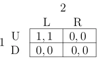
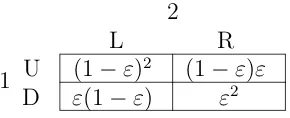
It is also important to note that implicit in Equation (4) above is that all players are randomising independently. There is also the concept of acorrelated strategy due to Aumann (1974), whereby two-or-more players can “correlate” their behaviour using a public randomisation device, though we will not cover this in this course. The difference between the two is subtle. The following 2×2 example should help to demonstrate how the set of distributions over outcomes from independent randomisations is smaller than that when correlated randomisation is allowed.

(17)

Right. If player 1 randomises independently, then he assigns some probability, call itp, to Up, and hence (1−p) to Down. Similarly, suppose player 2 assigns probability q to Left and hence (1−q) to Right. There are only 4 possible outcomes and the probability of each outcome occurring is given in the matrix below.

1

2

Left Right

Up pq p(1−q)

Down (1−p)q (1−p)(1−q)

Thus the distribution over outcomes is completely characterised by the two numbers p and q. That is, when players are acting independently, the family of distributions over outcomes are completely parameterized by the numbers p and q. But there are 4 possible outcomes, so the set of all distributions over these outcomes requires three parameters to fully classify. This can be generalised to say that Qn_j=14(Sj) is always

“smaller” than 4(S), since the size of each set are Q

j=1(|Sj| −1) and Q

j=1|Sj| −1

respectively. (Formally, the first set looks only at “product measures”.)

Here are some reasons why randomisation is useful:

• It can raise a player’s security level. Look back to Matching Pennies (Example

2). Before randomisation was allowed, each player’s security level was -1. What is it now?

• It can increase the power of dominance, by expanding the set of dominated actions since there are now more strategies that each pure strategy may be dominated by. The following game demonstrates this. Let x denote the payoff that the row player gets from choosing “Down”. Let’s vary x and see how things change.

1

2 Left Right Up 10,0 0,10 Middle 0,10 10,0 Down x,2 x,2

Figure 1: Mixed Strategy Dominance

There are really only three cases:

· x <0: ‘Down’ is strictly dominated by both Up and Middle.

· x <5: ‘Down’ is strictly dominated a mixed strategy, but not by a pure strategy.

· x≥5: ‘Down’ is not strictly dominated by any strategy, pure or mixed.

(18)

From here on in, the term strategy will refer to a mixed strategy. Also, our notions of dominance and security levels from Definitions4-6 can easily be extended to include mixed strategies, and this is what I mean when I use these terms from now on.

Here a short exercise designed to get you to show that while mixed strategies are an important and useful extension, when looking for strictly dominant strategies, we can restrict attention to pure strategies.

Exercise 1. Prove that a player can have at most one strictly dominant strategy.

Exercise 2. Show that there can be no strategy σi ∈Σi such that for all si ∈Si and

s−i ∈S−i,

Ui(σi,s−i)> Ui(si,s−i)

i.e. show that a dominant strategy must be a pure strategy.

Note that Exercise2asks you to compare playeri’s utility against not all strategies of his opponents, but rather only the pure strategies. While we extended our notions of dominance to include mixed strategies, Exercise 3 in the following section gets you to show that restricting attention to opponents’ pure strategies is actually enough.

5

Iterated Deletion of Dominated Strategies

In the previous Section we argued that players should never take a strategy that is strictly dominated. Given that a player will never take a strictly dominated strategy, we can effectively eliminate strictly dominated strategies from consideration.6 (Note that ignoring strictly dominated strategies requires no assumptions on the information that a player with a dominated strategy has about the other players’ payoffs.)

The next step is a jump. We now suppose that not only does a player eliminate his own dominated strategies for consideration, he also supposes that other players eliminate their strictly dominated strategies too. (Note that this does require further assumptions. It requires that a player is not only rational, but also knows that his opponents are rational.) This round of deletion generates a “new” and potentially “smaller” game than we were faced with previously. Furthermore, provided there is knowledge that all players in the original game is rational, all players understand that strategies in the new game are the only ones that need be considered. But now, provided that the players are willing to reason further about what their opponents know, we can start the whole elimination procedure again. The game may even be reduced further, the reason being that a strategy that was not dominated before may now be dominated once the game is reduced. We can then perform this operation again and again. Because a game may be arbitrarily large, we may have to iterate an arbitrarily large number of times and hence we need to appeal to common knowledge of rationality.

(19)

We already saw this in Example4. Initially ‘Down’ was dominated for player 1 and no strategy was dominated for player 2. Thus in the first round of deletion, we can dispense with ‘Down’ for player 1. But now, given that player 1 will never play ‘Down’, we can see that ‘Right’ is dominated for player 2. So provided that player 2 knows that player 1 is rational, he can reason that player 1 will never play “Down”, and as such is justified in taking the action “Left”. We are thus left with only one strategy for each player, yielding the strategy profile (Up, Left).

Now let’s extend the analysis of this example to a general process that we can apply to all games.

Recall that we extended Definitions 4 and 5 to include mixed strategies. However, it turns out that while it is true from the perspective of player i that he must con-sider mixed strategies of his own, when evaluating his own strategies, he can still limit attention to pure strategies of the other players.

That is, when we want to test if strategyσi is strictly dominated by strategyσi0, we

can just consider pure strategies ofi’s opponents. This is because

Ui(σi0,σ−i)> Ui(σi,σ−i), for all σ−i ∈Σ−i

if and only if

Ui(σ0i,s−i)> Ui(σi,s−i), for all s−i ∈S−i

The following exercise asks you to show this.

Exercise 3. Show that playeri’s pure strategysi ∈Si is strictly dominated if and only

if there exists a strategy σ0_i ∈Σi, such that

Ui(σi0,s−i)> Ui(si,s−i), for all s−i ∈S−i

The following exercise asks you to show that if we can eliminate a pure strategy for player i, then we can also eliminate any mixed strategy that plays this strategy with positive probability.

Exercise 4. Show that if pure strategy si is strictly dominated for player i, then so is

any mixed strategy,σi, such that si ∈supp(σi).

Now let us introduce our first solution concept. We will construct a set of strategies that survive when there is common knowledge that nobody will ever take a strictly dominated strategy. This is the set of strategies that survive the iterated deletion of strictly dominated strategies.

Begin with the game Γ =nN,{Si} n

i=1,{Ui} n i=1

o

. Now defineS0

i :=Si, and for each

k≥1, form the game Γ(k), with the same players, same utility functions, and strategy spaceS(k)_{, where}

S_i(k):=si ∈Si|si is undominated in Γ(k−1) , and

S(k):=

n Y

j=1

S_j(k)

(20)

1. S(k)_⊆_S(k−1)_{, for all} _k.

2. S(k) _{is nonempty for all} _k.

3. There exists a k∗, such that S(k)=S(k∗) for all k ≥k∗.

Finally we can define the set S∞ as

S∞ := \

k≥1

S(k)

Here are some comments about the process we just defined:

1. “Rational” opponents avoid dominated strategies. Sophisticated agents expect their “rational” opponents to do the same. And hence the procedure iterates.

2. The process is finite for games with finitely many players and strategies. That is, the process stops after a finite number of rounds, yielding a set of “surviving strategies” that are the only “rational” ways to play the game.

3. The order of the process does not matter. That is, consider the following three processes.

• Say to all the players: “Throw away all your dominated strategies”. Then after everyone had done that, make the same statement again. etc.

• Say to player 1: “throw away your dominated strategies”. Then given what player 1 threw away, say the same thing to player 2. etc. And then once you get to playern, we go back to player 1, make the same statement again and continue the cycle until it stops.

• Same as the second process, but instead only let each player throw away 1 strategy in each round.

The point is that the order and speed of the process has no effect on the set of strategies that survive.

4. The specifics of the process, i.e. the order of deletion, often does matter for delet-ing weakly dominated strategies. The reason for this is that a strictly dominated strategy stays strictly dominated once it is deleted, whereas a weakly dominated strategy may no longer be weakly dominated after other strategies are deleted.

As an example consider the following game taken from Kohlberg and Mertens (1986):

L R

(21)

It is clear that both M and D are strictly (and hence weakly) dominated for row. Now let’s compare the situation when we delete D to that where we delete M. The reduced games are denoted a and b in Figure 2below:

L R

U 3,2 2,2 M 1,1 0,0

L R

U 3,2 2,2 D 0,0 1,1

a b

Figure 2:

When we delete D for row we get the reduced game in Figure 2a. In this reduced game, R is now weakly-dominated for column. So if we were to now remove R, we would be left with the strategy profile (U, L) as the prediction. However, if we delete M first (giving us the game in Figure 2b), and then remove the weakly dominated strategy L for row, then our prediction would be the strategy profile (U, R).

5. Some interesting games are “dominance-solvable”. (i.e. the process ends with each player having one strategy remaining.)

6. Many games are not dominance-solvable.

7. We have defined a decreasing sequence of games Γ(k) =

n

N,

n

S_i(k)

on

i=1,{Ui} n i=1

o

.

However, again I have been sloppy. In each game Γ(k)_{, for every player} _{i, the}

function Ui is actually the restriction of the original utility function to the new

(potentially smaller) domain S(k)_.

A famous example of a dominance-solvable game, as defined in point5above, is the Cournot competition model where firms compete on the amount of output they will produce. These output decisions are made simultaneously and independently of the other firm. The firms have market power in that output decisions affect the market price.

Example 9 (Linear Cournot). There is a market with two firms, Firm 1 and Firm 2. Each firmi∈ {1,2} simultaneously chooses a quantity qi, so that total supply is given

byQ=q1+q2. The market price is determined as P(Q) = P(q1+q2) = a−b(q1+q2).

When firm i producesqi, it costs c(qi) =cqi. Each firm’s profit is given by:

Ui(qi, q−i) =qi a−b(qi+q−i)

−cqi

= (a−c)qi −bq2i −bqiq−i

(22)

Naturally we assume that firms are profit maximisers. Begin with defining each firm’s “reaction” function, a mapping ri : [0,∞) →[0,∞), which specifies the optimal

quantity to produce given what the other firm is producing. Compute these using the first order conditions for an optimum, to get

q_i∗ =ri(q−i) :=

a−c 2b −

q−i

2 (5)

It is immediate that ri is decreasing in what the other firm produces, q−i. Now let’s

begin the iterative process. In then first iteration we have thatS0

i := [0,∞). But from

equation (5) above, we have that anything above ri(0) is a strictly dominated strategy.

This must be so since the other firm chooses at least 0. Thus, after the first round of deletion we have thatS1

i := [0, ri(0)].

Since the game is symmetric, we know that the other firm reasons the same, and so they will also choose to produce no more thanri(0). Thus, it is now strictly dominated

to produce anything less thanri(ri(0)), which I will abbreviate tor2i(0). So we conclude

that after two rounds of deletion, thatS2

i := [ri2(0), ri(0)].

Now you can see the pattern. In the third round, since the opponent is choosing to produce a minimum of r2

i(0), then it is dominated for the firm to produce more than

ri(ri2(0)) =r3i(0). And so we have that Si3 := [ri2(0), r3i(0)]. etc.

Thus we have a sequence of nested setsS_ik ∞_k=0, which, it can be checked, converge to a point. What is the point? Well, it can be checked,that for all k= 1,2, . . .,

rk_i(0) : =a−c b

_Xk

j=1

(−1)j−11 2

j

=−a−c

b

_Xk

j=1

− 1

2

j

The series defined above is a standard one and converges to 1/3 as k → ∞. Thus we have that

r∞_i (0) = a−c 3b

Note that this solution could also be attained by observing that the game is symmetric, and so it must be thatq₋∗_i =q_i∗, and plugging this in to equation (5) above.

6

Rationalizability

(23)

6.1

Best-Responding

So how can we predict what players will/should do? Well, a reasonable thing to suppose is that at every opportunity that a player gets to choose an action, that the self-interested player will choose whatever is best for themselves given what the others are choosing. This leads us naturally to the notion of abest response, which generalises the idea of the reaction function we had in Example9.

Definition 8. Say that strategy σ∗_i is a best response for player i if there exists a

σ−i ∈Σ−i such thatσi∗ solves

max

σi∈Si

Ui(σi,σ−i) (6)

Of course there is no need for the best response for player i to be single-valued. That is, there is no reason to suppose that a player always has a unique best response for each strategy profile of the population. To discuss this further we need to introduce the notion of a correspondence.

Definition 9. A correspondence Ψ :X Y is a mapping that specifies for each point x∈X, a set Ψ(x)⊂Y.

A correspondence, Ψ, can also be viewed as a point to set function, Ψ : X → 2Y. (where 2Y denotes the power set ofY.)

Now let us define the best-response correspondence.

Definition 10. Playeri’s, best-response correspondence, bri :Σ−i Σi, is given by:

bri(σ−i) := n

σi ∈Σi

Ui(σ,σ−i)≥Ui(σ

0

i,σ−i), for all σ0i ∈Σi o

(7)

While Definition 10 is defined for mixed strategies, pure strategies still play a very important role. Why? Well, expected utility is linear in the probabilities and so since we are solving a linear optimization problem, a solution must occur at one of the boundaries. In fact, any non-degenerate mixed strategy that is a best-response puts positive weight only on those pure strategies that are themselves best-responses.

Perhaps this is a good time to note that the set of best responses for player i, is the set of best responses for player i to any belief, no matter how idiotic, about how the other players in the game will play. In other words there are no restrictions placed on whatσ−i could be.

Strategy σi is never a best-response if there is no σ−i for which σi is a best

re-sponse. Or in terms of conjectures, if there is no belief that player i may hold about his opponents’ behaviour,σ−i, that justifies choosing σi.

6.2

Rationalizable Strategies

(24)

never a best response is strictly dominated. This is difficult to show but important to know.

In games with more than 2 players, there may be strategies that are not strictly dominated but are nonetheless never a best-response. Just as we did with strictly dominated strategies, we can define a process that iteratively deletes strategies that are never a best-response. The resulting set of strategies for a given player are referred to as his/her set ofrationalizable strategies.

Let us show how to construct this set.

Begin with the game Γ = nN,{Si}n_i=1,{Ui}n_i=1 o

. Now define R(0)_i := Si, and for

each k ≥ 1, form the game Γ(k)_{, with the same players, same utility functions, and}

strategy spaceR(k), where

R(k)_i :=si ∈Si|si is a best response to some σ−i ∈Rk−−i1 , and

R(k) :=

n Y

j=1

R(k)_j

This process has the following properties:

1. R(k) _⊆_R(k−1)_{, for all} _k.

2. R(k) _{is nonempty for all} _k.

3. There exists a k∗, such that R(k) ₌_R(k∗) _{for all} _k _≥_k∗_.

Finally we can define the set R∞ as

R∞ := \

k≥1

R(k)

Let’s now recap the differences between Rationalizability and IDDS.

1. R∞⊆S∞.

2. R∞=S∞ for 2-player games.

3. R∞6=S∞ in general.

4. S∞ = T∞, where T∞ is the set of strategies obtained by iterative deletion of strategies that are not best-responses to correlated strategies. (This is very similar to rationalizability, and the reason more strategies survive is that you can best-respond to more things.) There can be no correlation in 2-player games.

(25)

7

Nash Equilibrium

Rationalizability and IDDS were our first pass at examining solutions to games. While useful they have some drawbacks.

• Even for small games they can be hard to check since you

– need to construct a chain of justification (rationalizability)

– need to repeatedly reduce the game (IDDS)

• The beliefs that a player holds about the behaviour of others need not be correct. In this sense a particular prediction need not be self-enforcing, since one or more players may want to deviate.

• In many games, all strategy profiles are rationalizable (e.g. Matching Pennies from Example 2), and so it not clear what pattern of play one should expect.

So we seek a more refined solution concept. One way to proceed is to ask what properties we would like our solution concept to possess?7 _{A strong, but desirable,}

re-quirement is that the solution concept must not be self-defeating. That is, if players are aware of the theory, they should have no incentive to deviate from the recommendation of the theory.

In this Section we introduce precisely such a solution concept. Like rationalizability, each player’s choice is again required to be optimal given his/her belief about other players, but now we add the additional constraint that a player’s belief is required to be correct. Such a strategy profile is referred to as a Nash Equilibrium. Let’s build up to the main result by first stating the definition in terms of pure strategies.

7.1

Pure Strategy Nash Equilibrium

Definition 11(Pure Strategy Nash Equilibrium). A pure strategy profiles∗ = (s∗₁, . . . , s∗_i, . . . , s∗_n) is a Nash Equilibrium if for every i, and all si ∈Si,

Ui(s∗i,s

∗

−i)≥Ui(si,s∗−i) (8)

Note that each player is best-responding to the strategies that the other players actually take. This differentiates the concept from that of a simple best-response, be-cause a best-response can be to any pattern of behaviour of the other players, no matter how idiotic. This also differentiates it from the concept of rationalizability, which only required that players best-respond to some reasonable conjecture of others’ behaviour, but perhaps not the conjecture they actually form. Nash Equilibrium requires that

(26)

conjectures be correct. Implicit in this is that all players possess the same beliefs about what an opponent will do. Given that we have added an additional constraint, it should be clear that every pure strategy Nash Equilibrium is rationalizable, and so the concept of equilibrium will always offer at least a sharp prediction as rationalizability and often offers much shaper predictions.

A Nash Equilibrium strategy profile is self-enforcing: if everybody else is playing their component of the strategy profile then it is rational for each player to play their component of the profile. To say this another way, unilateral deviations do not pay. (Note however, that a unilateral deviation need not strictly lower a player’s payoff, it just can’t possibly raise it. There is the stronger definition of a Strict Nash Equi-librium that deals with this case. In a strict equilibrium, the weak inequalities of Equation8 for each player are replaced with strict inequalities.)

There are two standard ways to think of a Nash Equilibrium arising.

1. As the result of a long-run process. In other words, the solution concept captures the steady state of play of a game where players hold correct expectations about the other players’ behaviour and they then act rationally. This viewpoint does not attempt to examine the process(es) by which the steady state might be reached. (‘Evolutionary’ models and ‘learning’ models formalise this.)

2. As a recommendation of play by a third party. Suppose there is an external arbitrator. If this arbitrator recommended to each player to play their component of the strategy profile, and everybody believed that the others would play their component of the profile, then no player has any incentive to deviate.

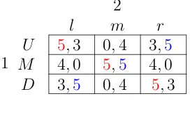
Let’s look at an example (taken from MWG page 246).

1

2

l m r

U 5,3 0,4 3,5 M 4,0 5,5 4,0 D 3,5 0,4 5,3

Figure 3:

(27)

Exercise 5. This is the the only equilibrium in this game, but there are lots more rationalizable strategy profiles. Find them.

7.2

Mixed Strategy Nash Equilibrium

The problem with pure strategy equilibria is that there are games for which one does not exist (Matching Pennies in Example 2 is the standard example), and failure of existence for a solution concept is a BIG, BIG deal. A solution concept is supposed to generate a prediction, and so, if it fails to exist then there are games about which we can predict nothing. And this is not good.

Fortunately, if we extend the notion of an equilibrium point to include mixed strate-gies, then we get existence.

Definition 12. A mixed strategy profile σ∗ = (σ₁∗, . . . , σ∗_i, . . . , σ∗_n) is a Nash Equilib-rium if for every i, and all σi ∈Σi,

Ui(σi∗,σ

∗

−i)≥Ui(σi,σ∗−i) (9)

Mixed strategy equilibria are at first difficult to interpret. The first reason, that we discussed before, is that mixed strategies are themselves difficult to interpret. The second reason is that a rational player will place strictly positive probability on two or more pure strategies (i.e. mix) in equilibrium only if he is indifferent between them. But given that these pure strategies yield the same payoff, first of all, why would the player randomise? And second, why would the player randomise in such a specific way? The answer is that he must do so in order to support the other players in playing their equilibrium strategies.

An example helps. Recall Matching Pennies. In the unique equilibrium to this game, each player randomises over their pure strategies with equal probability. But against an opponent who is randomising 50:50, both pure strategies yield the same payoff, so why would a player randomise in precisely this way given that they are indifferent? The answer, is that if the player does not randomise in this particular way, then the opponent will no longer be indifferent over his pure strategies and therefore won’t be willing to randomise himself. So, randomisation is used to keep the opponent indifferent, so that he is willing to randomise himself, and furthermore is willing to randomise in any and every possible way. But of course the same logic applies to the opponent. If he does not randomise in a very particular way, then the original player’s indifference is immediately broken and hence they are no longer willing to randomise. Thus, to keep the other guy indifferent, both players must randomise in precisely the correct way.

(28)

So finally, here is the most important result in Game Theory. It first appeared in Nash(1950, 1951).

Theorem 3. Every finiten-player normal form game,Γ =nN,{Si}n_i=1,{Ui}n_i=1 o

, has a mixed strategy Nash Equilibrium.

Two points are immediately worth noting about Theorem 3.

1. The Theorem only provides sufficient conditions for the existence of an equilib-rium. There may be games more general than those of Definition 2 that still possess equilibria. (There are, and we will see some later.)

2. The Theorem provides no clue as to what the equilibria may be. All we know is that at least one equilibrium exists, but the Theorem provides no indication as to how one might find it/them.

Let’s pause and mention a few things about Nash Equilibria for finite games.

• For finite games:

– A pure strategy Nash Equilibrium does not always exist.

– A Nash Equilibrium always exists (in mixed strategies).

• A Nash Equilibrium is rationalizable and survives IDDS.

(Hence a dominance solvable game possesses a unique Nash Equilibrium.)

• Games may have multiple Nash Equilibria. (see “Call Back” from Example 3.)

• While many games have multiple equilibria, almost all finite games have an odd number of equilibria.

• Nash equilibria need not be “good”, i.e. efficient. In fact they may be very ineffi-cient (see the Prisoners’ Dilemma).

• Nash Equilibrium payoffs are at least as great as the security level.

While the failure of existence of pure strategy Nash Equilibria for finite games may be unsettling, there is a class of infinite games that possess equilibria in pure strategies. These games are particularly useful for certain economic applications. The formal requirements for these games are as stated in the conditions of the following theorem, due toGlicksberg (1952).

Theorem 4. Let Γ = nN,{Si} n

i=1,{Ui} n i=1

o

be an n-player normal form game. An equilibrium exists in pure strategies if for all i∈ N,

1. Si is a non-empty, convex, and compact subset of some finite dimensional

(29)

2. the mapping Ui is continuous in s, and

3. for a fixed s∈S, the mapping s0_i 7→Ui(s0i,s−i) is quasiconcave.

There are many existence results available in the literature. There are also some ex-istence results for games with discontinuous payoffs (see Dasgupta and Maskin (1986), Simon and Zame (1990), and Reny (1999)). A good example of a game with discon-tinuous payoffs is an auction. Since if you lower your winning bid by just a tiny bit, it is possible that you will dramatically change the likelihood with which you win, thus changing your payoff substantially.

7.3

Proof of the Existence of Nash Equilibrium

This is a completely independent Section that proves the existence of a Nash Equilib-rium point for all finite games. It is optional and will not be examined.

Recall that a correspondence Ψ from X to Y is a function from X to subsets of Y. Of particular interest to game theorists, and economic theorists more generally, are correspondences from a set to itself that possess what is known as a fixed point.

Definition 13. A point x∗ ∈X is a fixed point of the correspondence Ψ from X to X if x∗ ∈Ψ(x∗).

A fixed point is an invariant point. That is, when the point is an input of the mapping, that same point is also an output. (Of course, since we are dealing with correspondences, this point may not be the only output.)

We will focus on a particular class of correspondences, that when defined on a space with some particular properties, possess a fixed point as guaranteed by Kakutani’s Theorem (Kakutani, 1941). Then we will show that the best-response correspondence is a member of this class of correspondences, and that the space of mixed strategies, Σ, is a space with the necessary properties. Since the best-response correspondence has a fixed point, there is at least one strategy profile that is a, though not necessarily unique, best-response to itself.

We need to build up to the statement of the existence Theorem. I try to minimise the amount of jargon as much as possible, but to do so entirely is unavoidable.

7.3.1 Metric Spaces

Definition 14. A metric space is a pair (X, d) where X 6=∅, and d: X×X → _R+

is a mapping that satisfies three conditions:

1. (symmetry) For all x, y ∈X, d(x, y) =d(y, x),

2. (distinguishes points) d(x, y) = 0 if and only if x=y,

(30)

Thus, a metric space is a set equipped with a well-defined, and often quite intuitive, notion of distance. An example of a metric space that is readily understood is X =

N:={. . . ,−2,−1,0,1,2, . . .} (the integers) and d(x, y) =|x−y|.

7.3.2 Limits, Completeness, Continuity, and Compactness8

A sequence in a set X is a mapping from _N to X. A typical sequence is denoted

{xn_}∞ n=1.

Definition 15. A sequence in a metric space (X, d) has a limit x if for every ε ∈_R+,

there exists andN ∈_N, such that for alln ≥N,

d(xn, x)< ε

This is written as xn →x and is often described as “xn converges to x”. The point x is also sometimes called a “limit point”.

LetF denote a nonempty subset of X, where (X, d) is a metric space. We say that F is aclosed setif for all sequences xn _in_F_{, if}_xn_→_x _then_x_∈_F_{. Thus, the set}_F _is

closed if it contains all of its limit points. A set G is open if its complement is closed. There are sets that are neither open nor closed so these two notions do not exhaust the class of all sets.

Theorem 5. The class of closed sets is closed under arbitrary intersections. That is, for a given index set A, if {Fα}α∈A is a collection of closed sets, then F :=∩α∈AFα is

a closed set. If A is finite, then F :=∪α∈AFα is closed.

We now define what are commonly referred to as the open balls. The open ball around point x with radius ε is defined asB(x, ε) := {y∈X :d(x, y)< ε}.

It can be shown that a set G is open if and only if for all x ∈ G, there exists an ε > 0 such that B(x, ε) ⊂ G. Thus for any point in an open set, we can construct a small set, specifically an open ball, around this point, such that all the points inside the open ball are still inside the original set. This result provides an intuitive image of an open set, since it means that if you are at a point in an open set you may move around a small bit in any allowable direction and still be inside the set. You can think of closed sets as having the opposite property in that you can get right to the boundary.9

Definition 16. Let (X, d) and (Y, ρ) be two metric spaces. A function f : X →Y is continuous at pointx if xn _→_x _implies _f(xn₎_→_f_{(x). A function is}_continuous _if

it is continuous at every point.

Note that the convergence of the sequence xn is with respect to the metric d, while convergence of the sequence f(xn_{) is with respect to the metric} _ρ.

The more general definition of continuity is via open and closed sets.

8_{I am omitting notes on completeness. So these notes are still quite incomplete} ,

(31)

Theorem 6. A function f :X →Y is continuous if and only if f−1_(G) _{is open in} _X_,

for every open G⊆Y.

We saw already that a sequencexninXis a mapping from_NtoX. Asubsequence ofxn_{is the restriction of this mapping to an infinite subset}_N0 _⊂

N. A subsequence is a

sequence in its own right. Typically a subsequence is defined asxnk_, _k∈

N. By writing

yk=xnk_{, we will say that the subsequence} _xnk _{converges if the sequence} _yk _converges.

Definition 17. A set F ⊂ X is compact if every sequence in F has a convergent subsequence and that subsequence converges to a point inF.

Note that the convergence must be to a point in F not just in X. Every compact set is closed, but not every closed set must be compact. For example the set [0,∞)⊂_R

is closed but not compact. A closed subset of a compact set is compact.

Theorem 7. A set F ⊂_R is compact if and only if it is closed and bounded.

So, finally we are getting there. All this is useful for the following two reasons. The first reason is that for a finite game, the sets Σi are all compact, and, by a famous result

known as Tychonoff’s Theorem, hence so is the setΣ:=Q

i∈NΣi.

The second reason is given in the following Theorem.

Theorem 8. If f is a continuous function on a compact set F, then there exists a nonempty, closed set of x∗ ∈F such that for all x∈F, f(x∗)≥f(x).

In words, Theorem 8 says that a continuous function on a compact set attains a maximum, and also says that the set of points that achieve this maximum is closed.

The final result on continuous functions concerns the mapping of a compact domain.

Theorem 9. IfF ⊂X is compact andf :X →Y is continuous, thenf(F)is compact. In particular, if X is compact, then f(X) is compact.

7.3.3 Correspondences

We are almost there! We just need a few properties of correspondences and then we can state Kakutani’s fixed point result. (Recall the definition of a correspondence from Definition9.)

Just as a function f can be identified by itsgraph, which is the collection of points

{x, f(x)}, a correspondence can be identified by its graph too. For a correspondence Ψ, the graph of Ψ,grΨ, is the set

grΨ :=

(x, y)y∈Ψ(x)

We are interested in correspondences that have closed graphs, i.e. in correspondences Ψ :X Y where the setgrΨ is closed. The definition in terms of sequences is,

Definition 18. The correspondence Ψ :X Y has aclosed graphif for any sequence

(32)

1. xn _∈_X _and _yn_∈_Ψ(xn_{) for every} _n,

2. xn →x∈X,

3. yn_→_y_∈_Y_,

then we have y∈Ψ(x).

Note that the bulk of Definition 18 comes from the three qualifiers. This has the effect of limiting the number of cases in which the conclusion y ∈ Ψ(x) is required to hold, and as a result the definition is not really that strong.

There is another, very similar, property of correspondences referred to as upper hemicontinuity. This is a slightly stronger condition than the closed graph property, though for our purposes the two will coincide.

Definition 19. The correspondence Ψ :X Y is upper hemicontinuous if 1. it has a closed graph,

2. the image of any compact set F ⊂X, Ψ(F), is bounded.

The second condition is what distinguishes Definition 19from Definition18, since a correspondence with only the closed graph property allows a compact set to be mapped to both open and closed sets, and it turns out that by adding the boundedness con-straint (condition 2 of Definition19), that the image of a compact set under an upper hemicontinuous correspondence is itself compact (so in fact, the boundedness implies closure).10 This is a property shared by continuous functions as we saw in Theorem 9, and is the reason either Definition 18or 19will work for our purposes (since Σ, which is itself compact, is both the domain and the range).

7.3.4 Existence

Here is the statement of Kakutani’s fixed point theorem that provides sufficient condi-tions for a correspondence to possess a fixed point.

Theorem 10(Kakutani’s Fixed Point Theorem).Suppose thatX ⊂_RN _{is a nonempty,}

compact, convex set, and that Ψ : X X is an upper hemicontinuous correspondence from X to itself, with the property that Ψ(x) is convex for all x∈X.

Then, Ψ has a fixed point.

(33)

We will now check that the best-response correspondence satisfies the hypotheses of Theorem 10. By Theorem 8 and the compactness of Σi, we have have that for all

σ, _BRi(σ) is a non-empty, compact subset of Σi. By linearity in its own strategies,

BRi(σ) is convex.

Combining all the players’ best-response correspondences, define BR:=×nj=1BRj.

We can check that the correspondenceσ 7→_BR(σ) that maps the non-empty, compact, convexΣ to itself, is

1. non-empty valued,

2. convex valued,

3. upper hemicontinuous (has the closed graph property).

So finally we can restate the main result that already appeared in Theorem3.

Theorem 11 (Nash). Every finite game has an equilibrium.

Our last result that completes this Section concerns the set of Nash Equilibria of a finite game. Denote the set of Nash Equilibria to a game Γ byE(Γ). Then,

Theorem 12. For a finite game Γ, E(Γ) is nonempty and closed.

The non-emptiness of E(Γ) was shown in Theorem 11. To see that E(Γ) is closed, define the set D:={(σ,σ)∈Σ×Σ}. If Σwas a 1-dimensional object, then the set D would just be the “diagonal”. Since BR is a correspondence from Σ to itself, the

set of fixed points of BR are the set of σ∗ such that (σ∗,σ∗) ∈ grΨ ∩D. The set

grΨ is closed by definition, and clearly D is closed as well. Thus, by Theorem 5, their

intersection is also closed.

8

Normal Form Equilibrium Refinements

In the previous Section we argued that if agents act independently, a satisfactory theory for rational play in games must prescribe a Nash Equilibrium. An obvious question to then ask is whether or not any Nash Equilibrium is a satisfactory recommendation of pla