Pintar2013-ChangePointDetection

Statistical methods for change-point detection in surface temperature

records

A. L. Pintar, A. Possolo, and N. F. Zhang

Citation: AIP Conf. Proc. 1552, 1048 (2013); doi: 10.1063/1.4819688

View online: http://dx.doi.org/10.1063/1.4819688

View Table of Contents: http://proceedings.aip.org/dbt/dbt.jsp?KEY=APCPCS&Volume=1552&Issue=1

Published by the AIP Publishing LLC.

Additional information on AIP Conf. Proc.

Journal Homepage: http://proceedings.aip.org/

Journal Information: http://proceedings.aip.org/about/about_the_proceedings

Top downloads: http://proceedings.aip.org/dbt/most_downloaded.jsp?KEY=APCPCS

Statistical Methods for Change-Point Detection in Surface

Temperature Records

A. L. Pintar, A. Possolo, and N. F. Zhang

Statistical Engineering Division Information Technology Laboratory National Institute of Standards and Technology

100 Bureau Drive Mail Stop 8980 Gaithersburg, MD 20899

Abstract. We describe several statistical methods to detect possible change-points in a time series of values of surface temperature measured at a meteorological station, and to assess the statistical significance of such changes, taking into account the natural variability of the measured values, and the autocorrelations between them. These methods serve to determine whether the record may suffer from biases unrelated to the climate signal, hence whether there may be a need for adjustments as considered by M. J. Menne and C. N. Williams (2009) “Homogenization of Temperature Series via Pairwise Comparisons”, Journal of Climate 22 (7), 1700–1717. We also review methods to characterize patterns of seasonality (seasonal decomposition using monthly medians or robust local regression), and explain the role they play in the imputation of missing values, and in enabling robust decompositions of the measured values into a seasonal component, a possible climate signal, and a station-specific remainder. The methods for change-point detection that we describe include statistical process control, wavelet multi-resolution analysis, adaptive weights smoothing, and a Bayesian procedure, all of which are applicable to single station records.

Keywords: Adaptive Weights Smoothing, Autocorrelation, Bayesian Methods, Bootstrap, Change-Point, Control Charting, Temperature Series, Wavelets.

INTRODUCTION

We describe several graphical, exploratory data analytic methods that indicate possible change-points in a time series of measured values of surface temperature at an observing station, and supplement them with statistical methods to confirm the reality of change-points, taking into account the natural variability of the measurements: all intended to serve as complements to the techniques described by [1].

We regard the sequence

1,..., n

t t

x x of measured

values of temperature made at nepochs t1,...tn(for

example, months), typically equispaced in time, as a

realization of a collection of random variables

1,..., n

t t

X X , which usually exhibit dependencies, and

are referred to collectively as a stochastic process. A change-point is an epoch t_ksuch that the joint probability distribution of

1

,...,

k m k

t t

X X is different

from the joint probability distribution of ,...,

k k m

t t

X X ,

for some mt1. This difference may take any of

several aspects, and possibly more than one aspect in conjunction, for example: a step change in mean value; an increase in variance; a change in the rate at which

the mean varies with time; an alteration of the auto-correlation function.

At most stations, the series of measured values of surface temperatures exhibits a strong pattern of seasonality. For example, for the record of monthly average maximum temperatures at a station at the Reno Tahoe International Airport, NV, about 92 % of the variability is due to oscillations driven by the changing seasons. Therefore, the pattern of seasonality, together with superimposed natural

“noise” (about 5 % of the variability at Reno), may

easily mask other changes. The section on seasonality describes techniques to estimate the seasonal component in a temperature record.

Typically, some of the data are missing, either sporadically, or at multiple observation epochs in succession: for example, for the Reno station, the value for August, 1900 is missing, but the values for adjacent months are available; for a station in Decatur, IL, the values are missing for all the months from November, 1985, until July, 1986. Since some techniques used either to estimate the seasonal component, or to detect change-points, can most easily be applied if no data are missing, the imputation of missing values is also discussed.

Many of the techniques that have been proposed for change-point detection neglect the fact that surface

temperature records typically exhibit non-negligible autocorrelations, even after removing temporal trends

and seasonal oscillations – [2] is a notable exception.

In general, such neglect leads to the identification of more change-points than in fact there are. In [3], a similar shortcoming related to the confirmation of a trend that has been detected using exploratory data analysis is discussed.

In the following sections we illustrate techniques for detecting and removing seasonality, imputing missing values, and detecting step changes in the mean. All of the change-point detection procedures that we discuss are sensitive to changes in the mean level of the process, and they explicitly account for autocorrelation.

SEASONALITY

Seasonal Decomposition Using Medians

A very simple, but quite effective estimate of the seasonal component reduces to finding the median temperature of the values pertaining to each month. This may be adapted to address a possibly temporally varying seasonality by computing monthly medians over a moving window of suitable length. This simple estimate can be computed even when there are many missing values.

Seasonal Decomposition Using Local

Regression

The method introduced by [4], and implemented in

the R [5] function stl, decomposes the series of

observations as xt mt st rt, where {mt}denotes a

trend, { }s_t a seasonal component, and { }r_t a

“remainder”, and does this by an iterative process

involving the application of the loess smoother [6].

Both the trend and the seasonal component are estimated in a way that is resistant to outlying observations. The procedure can be implemented to

tolerate missing data: since the current version of stl

does not do this, missing values should be imputed prior to its application. The seasonal component itself may vary throughout the time spanned by the series.

IMPUTATION

There are seven missing values in the series of maximum monthly temperatures for the Reno station, which were imputed using the following procedure:

1. Compute st, the median of the values

measured for all the months with the same

name as the month that t belongs to, in all

the years in the station’s record;

2. Fit a local regression model [7, 8] to the

observations in a two-year window

centered at t, (yet that obviously cannot

extend beyond the beginning or the end of

the record, if t should be near either of

them) and let xˆ_tdenote the value

predicted by this model for the value at

epoch t;

3. If the missing value occurs at epoch t that

is neither the first nor the last epoch on record, and it corresponds neither to the warmest month nor to the coldest month (as judged by the medians of the observations made in the same month of all years in the series), then impute the

missing value by xˆ_t;

4. Otherwise, impute the missing value by

ˆ

(stxt) 2.

The procedure just described may produce unrealistic imputations when there are runs of missing values spanning more than one half of the period of the seasonal oscillations, as there are in the record for a station in Decatur, IL. In such cases, the safest imputation foregoes interpolation and uses medians of monthly measured values.

STATISTICAL PROCESS CONTROL

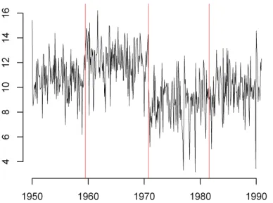
To illustrate techniques to be discussed in the following sections we will use a fragment of the

“remainder” component of the record for Reno, obtained applying the methods described in the sections about seasonality and imputation, modified to include three change-points defined by a shift in the

mean, of sizes V , 2V, and V 2, where V is the

standard deviation of the innovations of an auto-regressive moving average (ARMA) model [9] fitted

to that “remainder”: This is depicted in Fig. 1 where the vertical lines mark the change-points.

The EWMA (exponentially weighted moving average) chart described in section 6.3.2.4 of [10], commonly used in process quality control, can detect deviations in the mean of a time series. The EWMA statistics for a time series

1, 2,...

t t

x x is a time series

itself

1, 2,...

t t

z z where

1

(1 )

i i i

t t t

z

O

x

O

z for

2,3,...

i and for some 0d dO 1(O= 0.2 being a

common choice).

FIGURE 1. Change-Point Example — Data. This series, originally without change-points, was modified to include three change-points defined by a shift in the mean, of sizes V , 2V, and V 2, where V is the standard deviation of the innovations of the ARMA model fitted to that “remainder” series for Reno. The vertical lines show the true change-points.

mean, typically of the form

P

r

L

V

_z, where P

denotes the mean of {Xt}and

2

z

V denotes the limit that

the variance of the random variable Z_tconverges to as

t grows large.

The value of Vzdepends markedly on whether the

random variables {Xt}exhibit autocorrelation. In

[11], a practical approximation for

V

z2 is established

on page 28 assuming the {Xt} form a stationary

process with

V

2

as their common variance and

U

as

their auto-correlation function. In practice,

V

2 and

U

are estimated by a portion of {X_t} that is believed

to be stationary. The mean,

P

must be re-estimated

after each identified change, but the width of the control strip will remain the same unless one believes

2

V

and

U

have also changed.

Fig. 2 shows the results of applying this procedure

to the example series introduced above, with O=0.2

and

L

3

.

3

corresponding to a 99.9% normal

confidence interval. The series

{

Z

_t

}

identifies all

three change points but with a long delay for the third (more than three years). This delay is not surprising since the last change is small relative to the overall noise. The delay for detecting the first two larger changes is much shorter (a few months for the first and essentially none for the second). Such delays can be

influenced by the choice of O, which acts as a

dampening factor for how the changing mean affects

the level of

{

Z

_t

}

.

FIGURE 2. Change-Point Example — EWMA. The jagged line depicts the data, and the black dots represent the values of the EWMA statistic { }

i t

z computed using function

ewma defined in the R package qcc [12]. The vertical lines mark the locations of the three change-points that were introduced deliberately. The horizontal dashed lines mark the boundaries of the control strip, shifted after each change-point to facilitate identifying the next one.

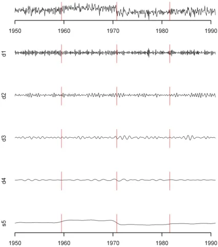
MULTI-RESOLUTION ANALYSIS

Fig. 3 shows the components of an additive

decomposition, multiresolution analysis (MRA)

[13],of the example time series introduced in Fig. 1: each of these components is a projection of the series onto a wavelet basis, and reveals how this time series varies at a particular scale.

The decomposition was computed using the

function mra of the package waveslim [14] for the

R environment for statistical computing, and it is based on the discrete wavelet transform corresponding to the least asymmetric wavelet LA(8) in [15] and periodic boundary conditions as described in section 4.6.3 of [16].

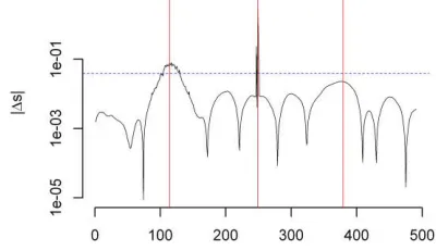
Fig. 4 serves as a diagnostic tool for the presence of change-points corresponding to shifts in the level of the series (it can be suitably adapted to become sensitive to other kinds of change-points). Since the

MRA segregates such shifts to the “smooth”

component s₅, we focus on the absolute values of the

corresponding first differences {st,5st1,5}. To

answer the question of how tall a peak needs to be to indicate a change-point with high confidence, we employed the following parametric bootstrap [17] procedure:

1. Perform a seasonal decomposition of the

series, and develop a statistical model for

the “remainder” (as defined in the section

example, a Gaussian ARMA(2,2) model proved adequate;

2. Choose a suitably large number m of

series to be simulated from the fitted

model — in our case we chose m =1000

— and for each of them compute the

MRA, and find the maximum absolute value of the first differences of the

“smooth” component;

3. The 95th percentile of this sample of m

maxima is an approximate threshold for

identification of change-points —

indicated by the horizontal, dashed (blue) line in Fig. 4.

In Fig. 4, the vertical lines mark the locations of the three change-points that were introduced deliberately, the dashed line marks the threshold above which first differences are considered to be change points, and the solid lines depicts the first differences. In this case, only one of the three change points is detected.

FIGURE 3. Change-Point Example — MRA. The top panel depicts the data, and the bottom five depict the components of a multi-resolution analysis (MRA) that expresses the data as the sum of a “smooth” (s5) and four levels of “detail” (d1–d4). All six panels have the same vertical scale. The vertical lines mark the locations of the three change-points that were introduced deliberately.

ADAPTIVE WEIGHTS SMOOTHING

Adaptive weights smoothing (AWS) [18] is a procedure that was originally conceived to detect discontinuities in digital images, hence to perform image segmentation, without blurring those

FIGURE 4. Change-Point Example — MRA Detection. The solid undulating curve depicts the absolute values of the first differences {s_t,5s_t1,5}of the “smooth” component of the MRA of the data. The horizontal dashed line indicates the 95th percentile of the reference distribution: excursions above this threshold indicate change-points.

discontinuities by over-smoothing. The procedure is non-parametric (that is, does not make assumptions about the probability distribution of the noise contaminating the signal that it seeks), and is adaptive (that is, its specific definition is driven by the data it is applied to).

The propagation-separation approach to AWS [19]

is implemented in function aws defined in the R

package of the same name [20], and can be applied not only to two-dimensional images, but also to time series. Fig. 5 depicts the results of applying the AWS algorithm to the example time series.

To assess the presence of a change-point, a procedure that is similar to the one used for MRA can be applied here, and its results are depicted in Fig. 6, which shows that two of the three change-points that are present in the example data set are identified. Since the MRA approach identified only one of the three change-points (see Fig. 4), the AWS approach performs better for the example data set. Actually, it is not too surprising that the rightmost change point is not be detected for either procedure because its size is one half of the typical size of the noise.

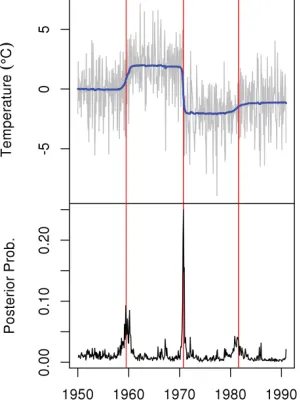
BAYESIAN CHANGE-POINT

DETECTION

In [21] a Bayesian approach is developed to determine the posterior probability of a mean shift at

each epoch assuming that { }

i t

X is an autoregressive

process of order p. More specifically, Xt_i

P

t_irt_i,

where

1

i i i i

t t t t

P

P

G E

and

1

i i j i

p

t j t t

j

r

¦

Ir a with the

} {

i t

FIGURE 5. Change-Point Example — AWS. The jagged thin line depicts the data, and the thick, generally smooth line depicts the trend detected by AWS. The vertical lines mark the locations of the three change-points that were introduced deliberately.

FIGURE 6. Change-Point Example — AWS Detection. The solid, undulating curve depicts the absolute values of the first differences {st st₁}of the smooth trend estimated by

AWS. The horizontal dashed line indicates the 95th percentile of the reference distribution: excursions above this threshold indicate change-points. Note that the vertical axis has a logarithmic scale.

random variables with probability H of being equal to

1 and the { }

i t

a independent and identically distributed

Gaussian random variables with mean 0 and standard

deviation Va. The autoregressive part of the model is

found in the definition of

i t

r since

i t

r depends on

1 i t r , 2 i t r

, , rti p . The

I

j are the dependence parameters

of this autoregressive process. The { }

i t

G and { }

i t E

allow for the possibility of a change-point, and they are interpreted as follows. If

i t

G

= 1, a change-point of

size

i t

E

exists at time ti, and if

G

ti= 0 there is no

change-point at time ti. Thus, to investigate the

possibility that a change-point exists at time ti, one

must calculate the probability that 1

i t

G conditionally

on the observed data, { }

i t

X . This is exactly the

posterior expected value of

i t

G

, which makes the

Bayesian paradigm of inference a natural fit.

By using conjugate forms for the prior distributions (see [21]), a Gibbs algorithm [22] can be constructed to sample from the joint posterior distribution of all of the parameters. Those samples are then used to estimate the properties of any marginal posterior distribution that is of interest. For example, the simple arithmetic average of the sampled values of

i t

G

(for

some ti) is an estimate of the posterior expected value

of

i t

G

.

There is no set prescription for deciding that a

change-point exists at time ti. The user is given the

flexibility to decide what level of evidence (that is, how large of a posterior probability) is sufficient to claim the existence of one or more change-points for some sub-sequence of epochs. This flexibility is important since different situations may call for different decision rules. Note that one also must set the confidence level in the EWMA, MRA, and AWS approaches.

Fig. 7 depicts the raw data and results of this

procedure taking p=1. The thin jagged line in the top

panel of Fig. 7 depicts the data, and the smooth line in the top panel of Fig. 7 shows the posterior mean of

i t

P

at all times. In the bottom panel of Fig. 7, the posterior expected value of

i t

G

at each ti is depicted

by the jagged curve, which provides a graphical way to assess the presence of a change-point. The vertical lines depict the actual change-points. From Fig. 7, it is clear that the first two true change-points are identified since there is a large rise in the posterior expected values of the

i t

G

around them. This is not necessarily

the case for the third and final true change-point. While there is a sustained noticeable elevation in the posterior expected values of the

i t

G

around that

change-point, the largest spike is not too much larger than some other spurious spikes. The fact that the expected values of the

i t

G

remain consistently elevated

relative to the general baseline speaks more cogently in favor of this being a true change-point than does the magnitude of these spikes. Therefore, we conclude that the Bayesian methodology identifies all three of the change-points.

CONCLUSION

Before employing such methods, it was necessary to remove seasonality from the times series and impute missing values. The methods were illustrated using a time series that was modified by the deliberate introduction of three change-points. The EWMA chart and our graphical approach to identify change points for the Bayesian method indicate the presence of all three change-points, with the EWMA chart doing so with some temporal delay for the third and smallest change. The AWS method did not identify the smallest change, but it did identify the two larger ones. The MRA identified the largest change-point. Note that at lower levels of confidence, the MRA and AWS approaches might also have identified all three change-points. A strength and common theme of the detection methods we presented in this article is that they are applicable to a single series, and they recognize and allow for autocorrelation, which is often present in temperature time series even after removing seasonality.

FIGURE 7. Change-Point Example — Autoregressive Process. The Jagged line in the top panel depicts the data. The vertical lines mark the locations of the three change-points that were introduced deliberately. The thick, generally smooth line in the top panel represents the level of the time series. The jagged line in the bottom panel depicts the posterior probability of a change-point at each epoch. The increases in posterior probability around the vertical lines indicate that all three change-points are found.

REFERENCES

1. Menne, M. J., and Williams, C. N. Jr., Journal of Climate22, 1700-1717 (2009).

2. Lund, R., Wang, X. L., Lu, Q. Q., Reeves, J., Gallagher, C., and Feng, Y., Journal of Climate 20, 5178-5190 (2007).

3. Percival, D. B., and Rothrock, D. A., Journal of Climate

18, 886-891 (2005).

4. Cleveland, R. B., Cleveland, W. S., McRae, J. E., and Terpenning, I., Journal of Official Statistics, 6, 3-73 (1990).

5. R Development Core Team, R: A Language and Environment for Statistical Computing, Vienna: R Foundation for Statistical Computing, 1020, URL http://CRAN.R-project.org ISBN 3-900051070.

6. Cleveland, W.S., Grosse, E., and Shyu, W. M., “Local Regression Models,” in Statistical Models in S, edited by J. M. Chambers, and T. Hastie, Pacific Grove: Wadsworth & Brooks/Cole, 1992, pp. 309-376.

7. Cleveland, W. W., and Devlin, S., J., Journal of the American Statistical Association83, 596-610 (1988). 8. Loader, C., Local Regression and Likelihood, New York:

Springer-Verlag, 1999.

9. NIST/SEMATECH, NIST/SEMATECH e Handbook of Statistical Methods, Gaithersburg: National Institute of Standards and Technology, U. S. Department of

Commerce, 2006, URL http://www.itl.nist.gov/div898/handbook.

10. Box, G. E. P., and Jenkins, G. M., Time Series Analysis, Forecasting, and Control, Oakland: Holden-Day, 1976. 11. Zhang, N. F., Technometrics 40, 24-38 (1998).

12. Scrucca, L., R News 4/1, 11-17 (2004), URL http://CRAN.R-project.org/doc/Rnews/.

13. Percival, D. B., and Walden, A. T., Wavelet Methods for Time Series Analysis, Cambridge: Cambridge University Press, 2000, pp. 65.

14. Whitcher, B., waveslim: Basic wavelet routines for one-, two- and three–dimensional signal processing, 2010, URL http://CRAN.R-project.org/package=waveslim, R package version 1.6.4.

15. Daubechies, I., “Ten Lectures on Wavelets” in Volume 61 of CBMS, NSF Regional Conference Series in Applied Mathematics, Philadelphia: Society for Industrial and Applied Mathematics, 1992.

16. Gencay, R., Selcuk, F., and Whitcher, B., An Introduction to Wavelets and Other Filtering Methods in Finance and Economics, San Diego: Academic Press, 2002.

17. Efron, B., and Tibshirani, R. J., An Introduction to the Bootstrap, New York: Chapman & Hall, 1993.

18. Polzehl, J., and Spokoiny, V., Journal of the Royal Statistical Society, 62, 335-354 (2000).

19. Polzehl, J., and Spokoiny, V., Probability Theory and Related Fields, 135, 335-362 (2006).

20. Polzehl, J., aws: Adaptive Weights Smoothing, 2010 URL http://CRAN.R-project.org/package=aws R package version 1.6-2.

21. McCulloch, R. E., and Tsay, R. S., Journal of the American Statistical Association88, 968-978 (1993). 22. Geman, S., and Geman, D., IEEE Transactions on