www.ann-geophys.net/28/515/2010/
© Author(s) 2010. This work is distributed under the Creative Commons Attribution 3.0 License.
Annales
Geophysicae
Communica
tes
Statistical analysis of the dependence of large-scale Birkeland
currents on solar wind parameters
H. Korth1, B. J. Anderson1, and C. L. Waters2
1The Johns Hopkins University, Applied Physics Laboratory, Laurel, MD, USA
2School of Mathematical and Physical Sciences, The University of Newcastle, NSW, Australia
Received: 24 September 2009 – Revised: 15 January 2010 – Accepted: 25 January 2010 – Published: 10 February 2010
Abstract. The spatial distributions of large-scale field-aligned Birkeland currents have been derived using magnetic field data obtained from the Iridium constellation of satellites from February 1999 to December 2007. From this database, we selected intervals that had at least 45% overlap in the large-scale currents between successive hours. The consis-tency in the current distributions is taken to indicate stabil-ity of the large-scale magnetosphere–ionosphere system to within the spatial and temporal resolution of the Iridium ob-servations. The resulting data set of about 1500 two-hour intervals (4% of the data) was sorted first by the interplane-tary magnetic field (IMF) GSM clock angle (arctan(By/Bz)) since this governs the spatial morphology of the currents. The Birkeland current densities were then corrected for vari-ations in EUV-produced ionospheric conductance by normal-izing the current densities to those occurring for 0◦ dipole tilt. To determine the dependence of the currents on other so-lar wind variables for a given IMF clock angle, the data were then sorted sequentially by the following parameters: the so-lar wind electric field in the plane normal to the Earth–Sun line, Eyz; the solar wind ram pressure; and the solar wind Alfv´en Mach number. The solar wind electric field is the dominant factor determining the Birkeland current intensi-ties. The currents shift toward noon and expand equatorward with increasing solar wind electric field. The total current increases by 0.8 MA per mV m−1increase inE
yzfor south-ward IMF, while for northsouth-ward IMF it is nearly independent of the electric field, increasing by only 0.1 MA per mV m−1 increase in Eyz. The dependence on solar wind pressure is comparatively modest. After correcting for the solar dy-namo dependencies in intensity and distribution, the total current intensity increases with solar wind dynamic pressure by 0.4 MA/nPa for southward IMF. Normalizing the
Birke-Correspondence to: H. Korth
land current densities to both the median solar wind elec-tric field and dynamic pressure effects, we find no significant dependence of the Birkeland currents on solar wind Alfv´en Mach number.
Keywords. Ionosphere (Auroral ionosphere; Electric fields
and currents; Ionosphere-magnetosphere interactions)
1 Introduction
Field-aligned Birkeland currents play a fundamental role in conveying stresses in the coupled solar wind– magnetosphere–ionosphere system. Determining the dominant physical quantities controlling these currents is therefore important for understanding the transport of elec-tromagnetic energy and momentum. The importance of the solar wind density and speed (Iijima and Potemra, 1982) and the interplanetary magnetic field (IMF) orientation (Potemra et al., 1984; Zanetti et al., 1984) in governing the Birkeland currents has been known for decades. Subsequent, compre-hensive observations from various single satellite studies combined with upstream solar wind and IMF measurements provided quantitative, two-dimensional distributions of the large-scale Birkeland currents. Statistical studies of magnetic field observations by the Dynamics Explorer 2 (Weimer, 2001, 2005) and the Ørsted (Papitashvili et al., 2002) satellites detailed the IMF dependence of the current distributions, revealing the IMF direction as the fundamental quantity determining the global-scale coupling geometry.
engineering magnetometer digitized to 30-nT resolution. For the period of this study these data were reported to the ground one vector magnetic field sample every 200 s on average. The temporal coverage of these observations is nearly continu-ous since February 1999. The Birkeland current distributions are calculated using Amp`ere’s law from fits of spherical har-monic basis functions to the observed magnetic perturbations (Waters et al., 2001). To resolve Birkeland currents to 4◦in latitude, a data accumulation over about one hour is required (Korth et al., 2004b, 2008). The Iridium data used here span
∼75 000 h of observations, allowing unprecedented statisti-cal analyses of the Birkeland currents and their dependence on solar wind parameters.
The Iridium database provides unique advantages for the statistical characterization of the Birkeland currents. Re-cently, Anderson et al. (2008), hereinafter denoted P1, com-piled statistical current distributions organized by IMF clock angle orientation. The statistical distributions were compiled from intervals with “stable” current topology obtained be-tween February 1999 and December 2005. The selection of data by stability in the analysis distinguishes this work from previous statistical studies (Weimer, 2001, 2005; Papi-tashvili et al., 2002), which required using data from all data intervals without regard to stability to obtain global obser-vational coverage. The topology of the Birkeland currents computed by averaging individual distributions derived from Iridium observations and sorted by IMF orientation agrees favorably with previous statistical analyses, but shows im-portant differences. For example, the influence of the IMF
By, which governs the direction of high-latitude flows arising from magnetopause reconnection, on the configuration of the dayside Birkeland currents is consistent with previous stud-ies conducted in the Northern Hemisphere. The effect of the sign of IMFByon the Birkeland current topology is reversed in the Southern Hemisphere due to the anti-symmetry of the reconnection site with respect to the noon-midnight merid-ian (Green et al., 2009). For southward IMF, the Birkeland current distributions derived from Iridium data do not show significant currents poleward of 80◦ MLAT, whereas some previous results show statistically significant NBZ-sense cur-rents (Zanetti et al., 1984) for all IMF orientations. Fur-thermore, for northward IMF, the Region-1 and particularly the Region-2 currents are much smaller in area and intensity compared to previous models. P1 suggested that the luxury of restricting the Iridium analysis to those intervals with rel-atively stable currents yields distributions that more nearly reflect pure states of the magnetosphere–ionosphere system. The results of P1 demonstrate the suitability of the Iridium stable-currents database for assessing the role of the IMF in governing solar wind–magnetosphere–ionosphere coupling. In this paper, this database is used to determine the influ-ence of the intensity on the solar wind electric field, dynamic pressure, and Alfv´en Mach number on the current distribu-tions and intensities. Ultimately these quantitative relation-ships can be applied to evaluate global geospace simulations,
in which the field-aligned current density is a fundamen-tal quantity, to determine what aspects of Birkeland current dynamics are best and least understood. The analysis de-scribed here is a step toward the ultimate goal of constructing a comprehensive model of the solar wind–magnetosphere– ionosphere interaction. The statistical analyses are described in Sect. 2. The results are discussed in Sect. 3 and summa-rized in Sect. 4.
2 Data analysis
2.1 Iridium database
This study uses Iridium data from February 1999 to Decem-ber 2007, two more years than used in P1. Iridium data were obtained for 97% of the days in this interval, yield-ing∼75 000 two-dimensional current patterns for analysis. The Iridium magnetometer samples were first reduced to magnetic perturbation data as described by Anderson et al. (2000). The Birkeland currents were then derived by fitting these perturbation data using a set of spherical harmonic ba-sis functions and applying Amp`ere’s law to the fit (Waters et al., 2001). The spherical harmonic fits were computed in a custom spherical coordinate system with the intersec-tion of the Iridium orbit planes at the pole. The results were transformed into Altitude Adjusted Corrected Geomagnetic (AACGM) coordinates (Baker and Wing, 1989), which are used throughout this manuscript. The maximum degree and order of the basis functions, and thus the spatial resolution of the current density, are prescribed by the spatial distribu-tion of the data samples. In azimuth, the smallest wavelength must be at least twice the longitude spacing between the or-bit planes,∼30◦. The latitude resolution afforded by the fit is a function of the magnetometer data sampling interval and the time over which data are accumulated. A sampling rate of one sample per 200 s from an individual satellite corresponds to a spatial along-track separation of∼12◦. The phasing of the magnetic field samples between satellites is random, and there are eleven satellites in each orbit plane, equally spaced along track, so the data point density along the orbit increases with time as samples from different satellites are made. For a one-hour data accumulation, the average spacing of the sam-ples is less than 12◦·9min/60min=1.8◦. This allows the Birkeland current distributions to be recovered with a lati-tude resolution of 4◦.
Elementary Current Method (ECM) (Amm, 2001), following P1, we restricted our analysis to the Northern Hemisphere Birkeland current observations.
Solar wind plasma (McComas et al., 1998) and IMF (Smith et al., 1998) observations by the Advanced Compo-sition Explorer (ACE) satellite at the first Lagrangian point, L1, were used to specify the solar wind/IMF conditions. For each one-hour Birkeland current distribution we averaged the ACE solar wind and magnetic field data for the time interval corresponding to simple advection delay between ACE and Earth. Since the intervals used are both long relative to errors in the advection time and correspond to stable IMF and so-lar wind properties (P1), this estimation for IMF conditions imposed on the system should be reliable.
2.2 Event selection
The magnetosphere can exhibit large-scale dynamics on time scales that are shorter than the one-hour accumulation times required to obtain Birkeland currents from the Iridium data used here. Care must therefore be taken in the selection of time intervals to be included in the analysis. Intervals were selected from the database for the statistical analysis using the method described in P1 to identify “stable” current dis-tributions. Briefly, this technique uses image object identifi-cation to locate the dominant upward and downward current regions in two consecutive one-hour distributions and then determines the fractional overlap of both the upward and the downward current regions between the two distributions. Re-quiring a fractional overlap of at least 45% ensured that the automatic procedure selected only those pairs of distributions that one would visually identify as consistent. The resulting stable-current intervals also correspond to stable conditions in the solar wind (P1). A total of 1536 events, correspond-ing to 4% of the database, met the selection criterion and have simultaneous observations of both IMF and solar wind plasma from ACE. Since plasma observations are available for a slightly smaller fraction of the time than IMF data, the fraction of suitable events available here is somewhat lower than in P1.
2.3 Conductance normalization
Systematic variations in ionospheric conductivity also change the Birkeland currents and the solar wind control of the currents must be distinguished from conductance effects. The two main sources of ionization are solar extreme ultravi-olet (EUV) radiation and energetic particle precipitation. The distributions of particle precipitation cannot be measured di-rectly and must either be inferred from auroral luminosities (Germany et al., 1989) or taken from statistical models de-rived from auroral (e.g., Zhang and Paxton, 2008) or precip-itation observations (e.g., Hardy et al., 1987, 1989). How-ever, the uncertainties associated with each of these methods are significant so that one risks introducing greater
system-atic errors by applying a correction than one might hope to remove. Moreover, the discrete precipitation is closely as-sociated with Birkeland currents, so that the distribution of currents and precipitation generally vary coherently. Conse-quently, introducing a statistical correction for particle pre-cipitation that does not move with the currents is likely to be worse than doing nothing. In the present analysis, we there-fore account only for changes in conductance due to solar illumination.
The Birkeland currents are affected primarily by the Ped-ersen conductance,6P, and Green et al. (2009) have shown that the current densities on the dayside are markedly re-duced during the winter months when the conductance due to solar EUV is generally lower. The solar EUV influence on6Pcan be expressed in terms of the solar zenith angle as (Rasmussen et al., 1988):
6P=4.5
1−0.85ν2 1+0.15u+0.05u2/B, (1) where ν=χ /90, u=F10.7/90, B is the magnetic field strength,F10.7is the 10.7-cm solar radio flux, andχ is the solar zenith angle. We normalized the dayside current densi-ties to equinox conditions by multiplying each Birkeland cur-rent distribution,ji(θ,φ), where the indexidenotes the event
number assigned to the current distribution, by the ratio be-tween the conductance distributions at equinox,6P,eq(θ,φ), and at the time of the observations,6P,i(θ,φ). The
normal-ized current density,ji∗(θ,φ)is given by:
ji∗(θ,φ)=ji(θ,φ)·6P,eq(θ,φ)/6P,i(θ,φ), (2) whereθ andφ are the magnetic colatitude and local time, respectively. For the equinox conductance distribution, we assume a solar radio flux ofF10.7=150×10−22Wm2Hz−1. Equation (1) is applicable within the solar zenith angle range 0◦≤χ≤85◦. Forχ >85◦, that is near the termina-tor and on the nightside, we do not anticipate a variation in conductance due to EUV so the normalization ratio should be set to unity there. To do this in a continuous way we first evaluated the minimum in6P,eqand in6Patχ=85◦. We then used the larger of these two minima as6P,minand set all values in6P,eqand6P that were below6P,min equal to
6P,min. The ratio 6P,eq/6P,i then transitions smoothly to unity at the terminator and the current densities on the night-side are unaffected by the normalization.
2.4 Solar wind electric field dependence
of the solar wind electric field,Eyz. For each of the distribu-tions we computedEyz=vp
q
B2
y+Bz2, wherevpis the pro-ton speed andByandBzare components of the IMF in GSM coordinates. The events within each αbin were separated by the magnitude ofEyzinto 1 mV m−1-wide bins centered atEyz=1, 2, 3, and 4 mV m−1. ForEyz>4.5 mV m−1, the number of events was insufficient for statistical analysis, so we restricted the study toEyz<=4.5 mV m−1, correspond-ing to low and moderate solar wind electric fields.
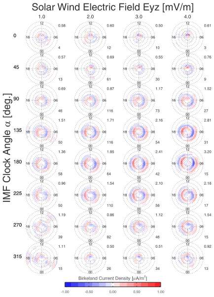
The average distributions within each (Eyz,α) bin are shown in Fig. 1. The rows and columns represent bins of the IMF clock angle and solar wind electric field magnitude, respectively. The average magnitude of the total current (top) and the number of events within each bin (bottom) are listed to the right of each distribution. The Birkeland total current was calculated as
Itot= 49 X
θ=1 23 X
φ=0
|j (θ,φ)|δA
2 , (3)
whereδA=R2iδφ δθsinθis the area element computed us-ingRi=6481 km for the radius of the ionosphere at an as-sumed altitude of 110 km,δφ=1h, andδθ=2◦. It is evident from Fig. 1 that the Birkeland current densities intensify for increasingEyzand this is reflected in the total current. This trend is stronger for southward than northward IMF. In ad-dition to the overall intensification of the Birkeland currents, the large-scale current regions obtained for southward IMF expand equatorward asEyzincreases.
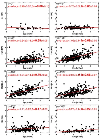
Figure 2 shows scatter plots of Itot versus Eyz for each current pattern sorted by IMF clock angle. The statistical de-pendence of the Birkeland total current onEyzwithin each
α-bin was estimated using a linear fit betweenItot andEyz. The electric fields considered here are less than values where saturation effects occur (Siscoe et al., 2002b; Ober et al., 2003; Anderson and Korth, 2007). The linear fits are shown in Fig. 2 including the corresponding fit parameters and un-certainties. The Birkeland total current increases with Eyz for all IMF clock angles. The linear fit slope depends on IMF orientation and is smallest for northward IMF, where the slope magnitude is less than the 1-σconfidence threshold (0.1 MA/(mV m−1)). The largest slope occurs for southward IMF (0.8 MA/(mV m−1)). The dependence of the Birkeland total current onEyzfor all IMF clock angle bins is summa-rized in the second column of Table 1.
The distributions in Fig. 1 also change withEyz. Figure 3 shows the current density along the dawn-dusk meridian for the fourEyzlevels in the 180° clock angle bin. An equator-ward expansion of the currents with increasingEyzis clearly evident.
[image:4.604.318.558.119.237.2]To quantify the influence ofEyzon the patterns, the aver-age distributions within each IMF clock angle bin for differ-entEyzmagnitudes were compared to theEyz=2 mV m−1 distribution for that clock angle bin. For this analysis we
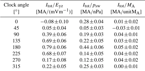
Table 1. Dependence of the Birkeland total current,Itot, onEyz, psw, and MA for different IMF clock angles. All uncertainties quoted are those of the 1-σconfidence level.
Clock angle Itot/Eyz Itot/psw Itot/MA
[◦] [MA/(mVm−1)] [MA/nPa] [MA/unitMA] 0 −0.08±0.10 0.28±0.04 0.01±0.02 45 0.05±0.04 0.05±0.03 −0.03±0.01 90 0.39±0.06 0.19±0.03 0.04±0.01 135 0.69±0.06 0.22±0.05 0.03±0.02 180 0.79±0.06 0.44±0.06 0.05±0.02 225 0.68±0.07 0.14±0.05 0.04±0.02 270 0.17±0.08 0.12±0.05 0.04±0.02 315 0.22±0.05 0.25±0.03 0.00±0.01
used the distribution of the average horizontal magnetic per-turbation,δB, rather than the current density. The smoother structure of the magnetic perturbations provides more stable root mean differences between patterns, and hence less noise in the differences between patterns, so that the shifts in the patterns can be computed more reliably.
In principle it is possible that changes in the location of the δB distribution can occur if only some of the currents change their locations. This might be the case for example if only the Region-2 currents shift equatorward with increasing
Eyz. If the latitude spanned by the current system does not change self-similarly with the equatorward displacement of the currents, this will show up as a systematic distribution in theδB residuals relative to the reference distribution. The
δBresiduals would then exhibit two rings, one poleward of the reference Region-1 currents, and the second equatorward of the reference Region 2 currents. Thus, by examining the 2-D magnetic perturbation residuals for systematic patterns we check for indications of such behavior. We note that the dawn-dusk meridian cuts in Fig. 3 do not show evidence of such behavior and none is found in the 2-D distributions ei-ther.
For this analysis the distribution forEyz=2 mV m−1was chosen as the referenceδBpattern and the grid positions of the magnetic perturbations for otherEyz distributions were parameterized with a colatitude expansion factor and off-sets in the midnight-to-noon and dawn-to-dusk direction. The best-fit latitudinal expansion factor and noonward and dawnward shift were determined simultaneously by mini-mizing the root-mean-square (rms) of the vector magnetic field residuals relative to the reference distribution.
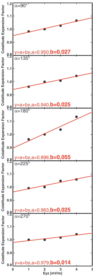
Figure 4 shows the colatitude expansion as a function of
Eyz for all IMF clock angle bins with Bz≤0 nT, and the expansion factors are summarized in the second column of Table 2. The currents expand equatorward with increasing
Solar Wind Electric Field Eyz [mV/m]
IMF Cloc
k Angle
[deg.]
a
00 06 12 18 4 0.58 0 1.0 00 06 12 18 12 0.60 0 2.0 00 06 12 18 10 0.50 0 3.0 00 06 12 18 3 0.61 0 4.0 00 06 12 18 13 0.57 45 00 06 12 18 61 0.69 45 00 06 12 18 30 0.55 45 00 06 12 18 9 0.76 45 00 06 12 18 46 0.69 90 00 06 12 18 116 0.87 90 00 06 12 18 73 1.17 90 00 06 12 18 27 1.52 90 00 06 12 18 50 1.51 135 00 06 12 18 116 1.71 135 00 06 12 18 54 2.16 135 00 06 12 18 31 2.81 135 00 06 12 18 58 1.36 180 00 06 12 18 64 1.85 180 00 06 12 18 42 2.41 180 00 06 12 18 15 3.20 180 00 06 12 18 50 0.96 225 00 06 12 18 110 1.54 225 00 06 12 18 56 2.10 225 00 06 12 18 17 2.18 225 00 06 12 18 39 1.19 270 00 06 12 18 82 0.86 270 00 06 12 18 46 1.12 270 00 06 12 18 15 1.54 270 00 06 12 18 15 1.11 315 00 06 12 18 26 0.50 315 00 06 12 18 34 0.51 315 00 06 12 18 13 0.92 3150 1 2 3 4 5 Eyz [mV/m]
0 2 4 6 8 10
I tot [MA]
α=0°
y=a+bx,a=0.96±0.26,b=−0.08±0.10
0 1 2 3 4 5
Eyz [mV/m] 0
2 4 6 8 10
I tot [MA]
α=45°
y=a+bx,a=0.75±0.09,b=0.05±0.04
0 1 2 3 4 5
Eyz [mV/m] 0
2 4 6 8 10
I tot [MA]
α=90°
y=a+bx,a=0.64±0.14,b=0.39±0.06
0 1 2 3 4 5
Eyz [mV/m] 0
2 4 6 8 10
I tot [MA]
α=135°
y=a+bx,a=1.05±0.14,b=0.69±0.06
0 1 2 3 4 5
Eyz [mV/m] 0
2 4 6 8 10
I tot [MA]
α=180°
y=a+bx,a=1.04±0.14,b=0.79±0.06
0 1 2 3 4 5
Eyz [mV/m] 0
2 4 6 8 10
I tot [MA]
α=225°
y=a+bx,a=0.81±0.16,b=0.68±0.07
0 1 2 3 4 5
Eyz [mV/m] 0
2 4 6 8 10
I tot [MA]
α=270°
y=a+bx,a=1.11±0.20,b=0.17±0.08
0 1 2 3 4 5
Eyz [mV/m] 0
2 4 6 8 10
I tot [MA]
α=315°
[image:6.604.133.479.67.548.2]y=a+bx,a=0.27±0.14,b=0.22±0.05
Fig. 2. Dependence of the Birkeland total current on the solar wind electric field,Eyz, and IMF clock angle,α. The parameters and 1-σ uncertainties of the linear fits (red lines) of these data are given at the top of each panel.
Birkeland currents for the IMF clock angle range 90◦≤α≤
270◦is 3%/(mV m−1). The shifts of the large-scale currents along the noon-midnight and dawn-dusk meridians are pre-sented in Fig. 5. Since the translation of the current pat-terns did not show a dependence on IMF clock angle a sin-gle linear function fits were estimated for the noonward and dawnward direction from all shifts evaluated in the clock angle range 90◦≤α≤270◦ at a particular Eyz level. We find that the currents shift toward local noon with
increas-ing Eyz by about 0.4◦/(mVm−1), with an uncertainty in the fitted slope of 0.1◦/(mVm−1) (cf. Fig. 5, top panel). On the other hand, the slope of fit for the dawnward shift, shown in the bottom panel of Fig. 5, is below the 1-σ con-fidence level. A shift in the dawn-dusk direction was thus not detected. Therefore, given the relative colatitude ex-pansion functions=1+0.03δEyz and noon shift function
60.0
18.0 40.018.0 20.018.0 0.06.0 20.06.0 40.06.0 60.06.0
-0.8 -0.6 -0.4 -0.2 0.0 0.2 0.4 0.6 0.8
Current Density [
µ
A/m
2]
Clat [deg] MLT [h]
1 mV/m 2 mV/m 3 mV/m 4 mV/m 180°, 18-06 MLT
[image:7.604.338.516.69.594.2]Fig. 3. Birkeland current density along the dawn-dusk (18:00– 06:00 MLT) meridian forEyz=1 (black), 2 (blue), 3 (green), and 4 mV m−1(red) in the 180° clock angle bin.
Table 2. Colatitude expansion factors of the Birkeland currents for Eyz, psw, andMA sorted by IMF clock angle. All uncertainties quoted are those of the 1-σconfidence level.
Clock angle Eyz psw MA
[◦] [%/(mVm−1)] [%/nPa] [%/unitMA] 90 2.7±0.3 3.7±0.5 1.3±0.2 135 2.5±0.4 1.2±1.1 0.1±0.5 180 5.5±1.1 0.7±0.2 −0.4±0.3 225 2.5±0.5 1.5±0.6 0.9±0.1 270 1.4±0.4 1.6±0.4 0.7±0.1
and local time,θandφ, is given by:
θ∗= q
s2θ2+2s θsin[15(φ−6)]+c2, (4)
φ∗=arctan s θ
sin[15(φ−6)]+c s θcos[15(φ−6)]
. (5)
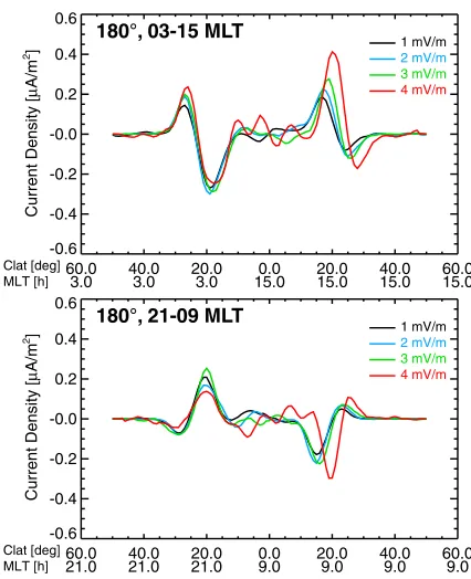
The shift of the large-scale currents toward noon is not im-mediately evident from Fig. 1. Figure 6 shows the Birke-land current density along the 03:00–15:00 MLT (top panel) and 21:00–09:00 MLT (bottom panel) meridians for eachEyz level in the 180° clock angle bin. The distributions used to evaluate these cuts were corrected for the equatorward ex-pansion of the Birkeland currents using the scale factor de-rived above. The latitudes of the nightside currents do not dependEyzbut the dayside currents move equatorward with increasingEyz, demonstrating the shift toward noon identi-fied above.
For IMFBz>0, colatitude expansion and noon shift can-not be determined reliably for two reasons. First, fewer events are available in each(Eyz,α)bin for these conditions, and the resulting statistical distributions are correspondingly less well defined so that the variance between distributions is dominated by the scatter and systematic trends are not appar-ent. Second, the Birkeland currents are concentrated at high latitudes and their areas are significantly smaller than for
0.8 0.9 1.0 1.1 1.2
Colatitude Expansion Factor
α=90°
y=a+bx,a=0.950,b=0.027
0.8 0.9 1.0 1.1 1.2 α
=135°
y=a+bx,a=0.940,b=0.025
0.8 0.9 1.0 1.1 1.2
Colatitude Expansion Factor
α=180°
y=a+bx,a=0.896,b=0.055
0.8 0.9 1.0 1.1 1.2
α=225°
y=a+bx,a=0.963,b=0.025
0 1 2 3 4 5
Eyz [mV/m] 0.8
0.9 1.0 1.1 1.2
Colatitude Expansion Factor
α=270°
y=a+bx,a=0.979,b=0.014
Colatitude Expansion Factor
[image:7.604.65.271.72.202.2]Colatitude Expansion Factor
Fig. 4. Dependence of the colatitude expansion factor on the solar wind electric field,Eyz, and IMF clock angle,α. The parameters and 1-σ uncertainties of the linear fits (red lines) of these data are given at the bottom of each panel.
[image:7.604.54.279.317.409.2]−1 0 1 2 3 4
Noon Shift [deg.]
y=a+bx,a=−0.72±0.27,b=0.39±0.10
90° < α < 270°
0 1 2 3 4 5
Eyz [mV/m] −1
0 1 2 3 4
Dawn Shift [deg.]
y=a+bx,a=0.02±0.14,b=0.01±0.05
[image:8.604.329.542.68.330.2]90° < α < 270°
Fig. 5. Noon-midnight (top panel) and dawn-dusk (bottom panel) translation as function of the solar wind electric field. The parame-ters and 1-σ uncertainties of the linear fits (red lines) of these data are given at the bottom of each panel.
relative spatial distributions, it turns out that the noise in re-gions without currents dominates the deviation so that the optimization algorithm fails to yield reliable results.
2.5 Solar wind dynamic pressure dependence
The solar wind pressure, for constant Eyz, affects the size of the magnetosphere (Sotirelis and Meng, 1999) and the magnetospheric plasma densities (Wing and Newell, 1998; Borovsky et al., 1998), both of which might be expected to influence the Birkeland currents. To analyze the influence of the solar wind dynamic pressure, psw, we first removed the dependence onEyzby normalizing the Birkeland current distributions to a meanEyzof 2.3 mV m−1using the relation-ships given in Sect. 2.4. The current patterns were separated into the IMF clock angle bins used above and then sorted by solar wind dynamic pressure within each IMF clock an-gle bin. The solar wind dynamic pressure was calculated as
psw=mpnpvp2, wheremp is the proton mass andnpis the proton density measured by ACE. The data set was binned by solar wind dynamic pressure in four one nPa-wide bins centered at 0.5, 1.5, 2.5, and 3.5 nPa.
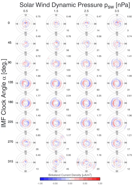
The average current patterns for each (psw,α) bin are shown in Fig. 7. There is an overall increase in the current densities with increasingpsw. The dependence of Birkeland
60.0
3.0 40.03.0 20.03.0 15.00.0 20.015.0 40.015.0 60.015.0 -0.6
-0.4 -0.2 -0.0 0.2 0.4 0.6
Current Density [
µ
A/m
2]
Clat [deg] MLT [h]
1 mV/m 2 mV/m
3 mV/m 4 mV/m
60.0
21.0 40.021.0 20.021.0 0.09.0 20.09.0 40.09.0 60.09.0 -0.6
-0.4 -0.2 -0.0 0.2 0.4 0.6
Current Density [
µ
A/m
2]
Clat [deg] MLT [h]
1 mV/m 2 mV/m
3 mV/m 4 mV/m
180°, 03-15 MLT
[image:8.604.58.294.71.335.2]180°, 21-09 MLT
Fig. 6. Birkeland current density along the 03:00–15:00 MLT (top panel) and 21:00–09:00 MLT (bottom panel) meridians forEyz=1 (black), 2 (blue), 3 (green), and 4 mV m−1(red) in the 180° clock angle bin. The colatitude is corrected for the equatorward expansion of the Birkeland currents.
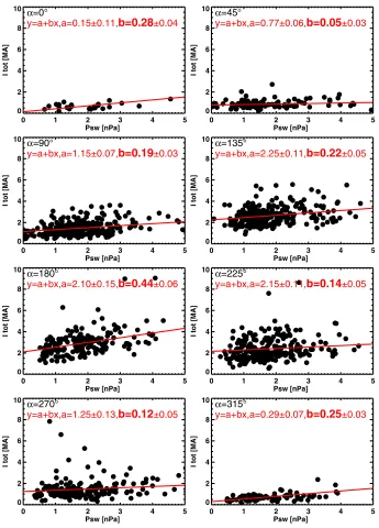
total current onpswis presented in Fig. 8, which shows the total current as a function of dynamic pressure in each IMF clock angle bin. The results are summarized in the third col-umn of Table 1. The linear trend lines show that the total current intensifies with increasingpsw, independent of IMF orientation. The maximum increase of the Birkeland total current per unitpswis about 0.4 MA/nPa for southward IMF while local minima are found for dawnward and duskward IMF orientation. The influence ofpswon the Birkeland cur-rent pattern is less evident. The factors for the equatorward expansion are shown in the third column of Table 2. Com-pared with the effect of the Eyz within a given clock an-gle bin having a non-zero southward IMF component, the equatorward expansions due to increases inpsware not only markedly smaller but also approach the confidence thresh-olds of the slopes from the linear trend lines. Nevertheless, the slopes are consistently positive and exhibit magnitudes above the 1-σ threshold so that the smallpsw-driven equa-torward expansion may be genuine.
2.6 Solar wind Alfv´en Mach number dependence
Solar Wind Dynamic Pressure p
sw
[nPa]
IMF Cloc
k Angle
[deg.]
a
00 06 12 18 3 0.75 0 0.5 00 06 12 18 10 0.48 0 1.5 00 06 12 18 14 0.47 0 2.5 00 06 12 18 3 0.92 0 3.5 00 06 12 18 28 0.49 45 00 06 12 18 56 0.76 45 00 06 12 18 21 0.58 45 00 06 12 18 10 0.74 45 00 06 12 18 51 0.72 90 00 06 12 18 123 1.00 90 00 06 12 18 72 1.05 90 00 06 12 18 14 1.41 90 00 06 12 18 32 1.68 135 00 06 12 18 131 1.92 135 00 06 12 18 60 2.10 135 00 06 12 18 31 1.99 135 00 06 12 18 33 1.77 180 00 06 12 18 83 2.04 180 00 06 12 18 45 2.25 180 00 06 12 18 18 2.61 180 00 06 12 18 45 1.49 225 00 06 12 18 108 1.63 225 00 06 12 18 62 1.77 225 00 06 12 18 17 1.96 225 00 06 12 18 26 0.85 270 00 06 12 18 77 1.17 270 00 06 12 18 52 1.05 270 00 06 12 18 17 1.21 270 00 06 12 18 13 0.40 315 00 06 12 18 45 0.95 315 00 06 12 18 20 1.16 315 00 06 12 18 12 0.73 3150 1 2 3 4 5 Psw [nPa]
0 2 4 6 8 10
I tot [MA]
α=0°
y=a+bx,a=0.15±0.11,b=0.28±0.04
0 1 2 3 4 5
Psw [nPa] 0
2 4 6 8 10
I tot [MA]
α=45°
y=a+bx,a=0.77±0.06,b=0.05±0.03
0 1 2 3 4 5
Psw [nPa] 0
2 4 6 8 10
I tot [MA]
α=90°
y=a+bx,a=1.15±0.07,b=0.19±0.03
0 1 2 3 4 5
Psw [nPa] 0
2 4 6 8 10
I tot [MA]
α=135°
y=a+bx,a=2.25±0.11,b=0.22±0.05
0 1 2 3 4 5
Psw [nPa] 0
2 4 6 8 10
I tot [MA]
α=180°
y=a+bx,a=2.10±0.15,b=0.44±0.06
0 1 2 3 4 5
Psw [nPa] 0
2 4 6 8 10
I tot [MA]
α=225°
y=a+bx,a=2.15±0.11,b=0.14±0.05
0 1 2 3 4 5
Psw [nPa] 0
2 4 6 8 10
I tot [MA]
α=270°
y=a+bx,a=1.25±0.13,b=0.12±0.05
0 1 2 3 4 5
Psw [nPa] 0
2 4 6 8 10
I tot [MA]
α=315°
[image:10.604.135.480.68.548.2]y=a+bx,a=0.29±0.07,b=0.25±0.03
Fig. 8. Dependence of the Birkeland total current on the solar wind dynamic pressure,psw, and IMF clock angle,α. The parameters and 1-σuncertainties of the linear fits (red lines) of these data are given at the top of each panel.
We therefore also examined the influence of the solar wind Alfv´en Mach number on the Birkeland currents. The Birke-land currents were normalized to mean values of both solar wind electric field, Eyz=2.3 mV m−1, and dynamic pres-sure,psw=1.75 nPa, using the linear trends presented above. The solar wind Alfv´en Mach number, MA, was calculated from ACE data asMA=vp/vA, where the Alfv´en velocity
vA=B/
√
µ0npmp was computed from the magnetic field intensity, B, and the proton mass,mp. The current patterns
current shows consistent increases for all but one IMF clock angle bin, one could infer, if anything, a minor increase in
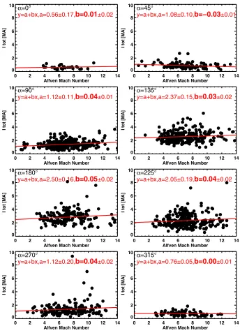
Itot with increasingMA. In addition, the colatitude expan-sion factors associated withMA (Table 2, fourth column), gave the smallest values in every clock angle bin indicating a very weak dependence. We conclude that the Iridium statis-tical distributions provide no evidence for significant control of the large-scale Birkeland currents by the solar wind Alfv´en Mach number.
2.7 Simultaneous multi-variable regression
The parameters we chose to represent the solar wind in-fluence on the magnetosphere were selected based on their physical roles in the magnetosphere–solar wind interaction. The clock angle is used because it plays a dominant role in controlling the location of magnetopause reconnection and hence on the configuration of the Birkeland currents. The solar wind electric field is the primary factor governing the intensity of reconnection and hence convection for a given clock angle. The solar wind ram pressure is the dominant factor determining the size of the magnetosphere, and finally the Alfv´en Mach number was included because it has been suggested that it plays a secondary role in the reconnection intensity by affecting the efficiency.
Despite these physical motivations, the last three param-eters, Eyz, psw, and MA are highly correlated in the solar wind. They all depend on the solar wind velocity. BothEyz andMAdepend on the IMF (thoughEyz is only dependent on two components of the magnetic field), and bothpswand
MAdepend on the solar wind density. It is therefore possible that in subtracting off the dependence ofItotonEyzand then the dependence onpswwe inadvertently removed a stronger dependence onMA giving a false impression of a weak in-fluence ofMA.
To test for the possibility that our analysis has masked dif-ferent dependencies than obtained above, we also used multi-variable regression to determineItotas a function of all three parameters simultaneously. For each clock angle bin we fit
Itotto the following:
F (Eyz,psw,MA)=m0+m1Eyz+m2psw+m3MA (6) using the formalism described in Korth et al. (2004a), which also yields estimates for the uncertainties in themi. The
re-sults are given in Table 3. Comparing these rere-sults with those given above in Table 1 we find broad agreement: theEyzand
pswcoefficients’ 1-σ ranges overlap in all cases except the 315◦clock angle bin, and theMAcoefficients are the small-est by a significant margin and in many cases the 1-σ range is consistent with zero. Thus, we obtain the sameEyz and
[image:11.604.311.547.130.245.2]pswdependencies and get the same result that the influence ofMAis weak, possibly even consistent with no statistically significant variation ofItotwithMA.
Table 3. Correlation coefficients between total Birkeland current, Itot, and solar wind electric field, Eyz, solar wind ram pressure, psw, and solar wind Alfv´en Mach number,MA, determined using simultaneous multiple linear regression.
Clock angle Itot/Eyz Itot/psw Itot/MA
[◦] [MA/(mVm−1)] [MA/nPa] [MA/unitMA]
0 −0.03±0.10 0.25±0.05 0.04±0.04 45 0.03±0.05 0.05±0.04 0.00±0.02 90 0.41±0.07 0.13±0.05 0.08±0.03 135 0.64±0.08 0.25±0.07 −0.00±0.03 180 0.67±0.07 0.39±0.06 −0.05±0.02 225 0.68±0.09 0.12±0.05 0.02±0.03 270 −0.02±0.12 0.24±0.07 −0.04±0.03 315 0.10±0.04 0.33±0.04 −0.03±0.01
3 Discussion
Statistical analysis of Birkeland current distributions derived from magnetic field observations by the constellation of Irid-ium satellites shows that the large-scale Birkeland currents are controlled most strongly by the IMF orientation and the solar wind electric field. The solar wind ram pressure exerts a secondary influence, and we found no effect from the so-lar wind Alfv´en Mach number. The correspondence between the Birkeland current patterns and the expected ionospheric projection of reconnection flows (P1) suggests that magne-topause reconnection is the dominant mechanism exercising control over the Birkeland currents. The strongest variation with solar wind conditions within a given IMF clock angle range is due to the solar wind electric field,Eyz.
Magnetic reconnection taps a fraction of the solar wind po-tential, providing the magnetospheric convection popo-tential,
φm, which is impressed on the ionosphere via equipotential magnetic field lines (e.g., Reiff et al., 1981). For nominal, that is not extreme, solar wind conditions considered in this study, the transpolar cap potential,φpc, is assumed to equal
φmso that the Birkeland current intensity is proportional to
φm. This assumption is not valid during active times when saturation effects come into play (Hill et al., 1976). In the non-saturated regime, magnetic reconnection implies that the Birkeland current density,jr, is related to drivers in the solar wind by (Siscoe et al., 2002a,b):
jr∼φm∼Eswpsw−1/6frF (α), (7) whereEswandpsware the solar wind electric field and dy-namic pressure, respectively, andfris the reconnection effi-ciency. The functionF (α), whereF (0◦)=0 andF (180◦)=
0 2 4 6 8 10 12 14 Alfven Mach Number
0 2 4 6 8 10
I tot [MA]
α=0°
y=a+bx,a=0.56±0.17,b=0.01±0.02
0 2 4 6 8 10 12 14
Alfven Mach Number 0
2 4 6 8 10
I tot [MA]
α=45°
y=a+bx,a=1.08±0.10,b=−0.03±0.01
0 2 4 6 8 10 12 14
Alfven Mach Number 0
2 4 6 8 10
I tot [MA]
α=90°
y=a+bx,a=1.12±0.11,b=0.04±0.01
0 2 4 6 8 10 12 14
Alfven Mach Number 0
2 4 6 8 10
I tot [MA]
α=135°
y=a+bx,a=2.37±0.15,b=0.03±0.02
0 2 4 6 8 10 12 14
Alfven Mach Number 0
2 4 6 8 10
I tot [MA]
α=180°
y=a+bx,a=2.50±0.16,b=0.05±0.02
0 2 4 6 8 10 12 14
Alfven Mach Number 0
2 4 6 8 10
I tot [MA]
α=225°
y=a+bx,a=2.05±0.19,b=0.04±0.02
0 2 4 6 8 10 12 14
Alfven Mach Number 0
2 4 6 8 10
I tot [MA]
α=270°
y=a+bx,a=1.12±0.20,b=0.04±0.02
0 2 4 6 8 10 12 14
Alfven Mach Number 0
2 4 6 8 10
I tot [MA]
α=315°
[image:12.604.134.478.68.545.2]y=a+bx,a=0.76±0.05,b=0.00±0.01
Fig. 9. Dependence of the Birkeland total current on the solar wind Alfv´en Mach number,MA, and IMF clock angle,α. The parameters and 1-σuncertainties of the linear fits (red lines) of these data are given at the top of each panel.
The dependencies of the Birkeland currents on the solar wind electric field identified in Sect. 2.4 agree with expecta-tions from reconnection. Figure 2 reflects the linear depen-dence of the total current and hence, the current densities on
Eyz implied by Eq. (7) for a wide range of IMF clock an-gles. The dependence varies with IMF clock angle and is largest for southward IMF and weakest for northward IMF, represented by the functionF (α)in Eq. (7). In Fig. 2, the dependence on Eyz is rather weak, the slopes for α=0◦
andα=45◦ are lower in magnitude than the associated
1-σuncertainties, indicating that the intensification withEyzis modest for northward IMF. However, we note that the cur-rent for extreme conditions and northward IMF (Korth et al., 2005; Merkin et al., 2007) is markedly larger than the events used here.
of weakly diminishing Birkeland current densities predicted by Eq. (7), the Iridium distributions show intensifications of
Itotwith increasing solar wind dynamic pressure for all IMF orientations.
An alternate means for transport of energy and momentum from the solar wind into the magnetosphere is viscous inter-action between the solar wind flow and the magnetospheric circulation (Axford and Hines, 1961). The magnetospheric plasma flow,v, driven by viscous interaction generates cur-rents,J⊥, perpendicular to the magnetic lines of force,B,
and field-aligned Birkeland currents,J||, arise from the
re-quirement for current continuity (e.g., Parks, 2004):
∇ ·J||= −∇ ·J⊥= −
B× ∇p
B2 −ρ
B
B2×(v· ∇)v. (8) In Eq. (8),pandρare the plasma pressure and mass density, respectively. The viscous dynamo is believed to be primarily driven by the Kelvin-Helmholtz instability caused by shear flows between the solar wind and magnetospheric plasmas at the magnetopause (Rostoker et al., 1987). For a tangential discontinuity in an incompressible magnetized plasma, the condition for instability of a wave propagating in directionkˆ
is given by (e.g., Landau and Lifschitz, 1960; Kivelson and Chen, 1995):
h
ˆ
k·(v2−v1)
i2
> ρ1+ρ2 µ0ρ1ρ2
B1·kˆ
2
+B2·kˆ 2
, (9)
whereµ0is the vacuum permeability and the indices 1 and 2 represent the two sides of the discontinuity. Assuming that the Kelvin-Helmholtz waves travel anti-sunward, the insta-bility condition Eq. (9) is most readily satisfied for purely northward or southward IMF direction, for which the draped magnetosheath field at the flanks has no component in the flow direction. The viscous interaction thus might be ex-pected to be favored under these conditions leading to a stronger dependence of the Birkeland currents on solar wind conditions. This expectation is consistent with the statisti-cal analysis shown in Fig. 8. The Iridium observations yield persistent positive correlations between the Birkeland total current andpswas one would anticipate if the field-aligned current intensity is modulated by the solar wind flow ve-locity for a fixed electric field. (Recall that theEyz depen-dence was removed in the pressure analysis.) Furthermore, the Iridium observations exhibit local minima for dawnward and duskward IMF in the influence of ram pressure on the Birkeland total current consistent with Eq. (9). This indi-cates that the viscous interaction drives at least a portion of the Birkeland currents.
Finally, we consider the implications of the lack of signif-icant influence of the solar wind Alfv´en Mach number. The reconnection efficiencyfrin Eq. (7) is defined as the ratio of the inflow velocity from the magnetosheath into the re-connection line, vr, and the Alfv´en velocity, vA (Petschek, 1964). Determining the value offris difficult because it de-pends on assumed boundary conditions and on the locations
wherevr andvA are measured (Sonnerup, 1974). Further-more, Sonnerup (1970) argued that reconnection should be entirely absent in high-βplasmas, whereβ=2µ0p/B2is the ratio of gas pressure to magnetic pressure. Indeed, previous observations consistently link increases in the plasma β to decreased reconnection efficiency (Paschmann et al., 1986; Scurry et al., 1984; Phan et al., 1996). This finding was in-dependently confirmed by Anderson et al. (1997) from com-parison of AMPTE/IRM and AMPTE/CCE observations of plasma depletion in the subsolar quasi-perpendicular mag-netosheath. Because the geocentric distance for apogee of these spacecraft, 8.8REfor CCE and 18.8REfor IRM, dif-fer significantly, the spacecraft encounter the magnetosheath for distinct ranges in the solar wind Alfv´en Mach number. From the relative difference in the reconnection efficiency identified in the two sets of observations, Anderson et al. (1997) inferredfr∼1/βshforβsh>1 measured in the mag-netosheath. Assuming a quasi-perpendicular bow shock in the strong shock limit for whichβsh=3/32MAsw2 , these au-thors further correlatefr with the solar wind Alfv´en Mach number,MAsw:
fr∼ 1
βsh
∼ 1
MAsw2 . (10)
Relation (10) predicts the reconnection efficiency and, there-fore, the Birkeland total current to be strongly anti-correlated with solar wind Alfv´en Mach number. Instead, the statisti-cal analysis presented in Fig. 9 showed, if anything, a slight positive correlation of the current withMAsw. The analysis presented here is for modest forcing, i.e., lowMAswandβsh, such that the reconnection efficiency changes are not evident for the range of forcing represented by this data set. Exam-ination of extreme conditions may be needed to reflect the influence of decreasing reconnection efficiency, but it is not a determining factor for the nominal ranges of forcing con-sidered here. It may be that the decreases in reconnection efficiency do not reduce the solar wind dynamo potential im-posed on the M–I system so long as the reconnection flows can accommodate the imposed solar wind flow. Only when the imposed solar wind flow exceeds the flow that reconnec-tion can accommodate will the variareconnec-tion in reconnecreconnec-tion ef-ficiency be evident. We therefore conclude that for nomi-nal conditions, the reconnection efficiency is more than suf-ficient to take up the imposed solar wind flow. The decrease in reconnection efficiency is therefore an effect that does not come into play for the range of solar wind forcing considered here.
the magnetotail (Siscoe and Huang, 1985). When the solar wind electric field increases, so does the reconnection rate at the dayside magnetopause while that in the magnetotail re-mains initially unchanged. The polar cap then responds to the increase in open magnetic flux by expanding equatorward. Since Region-1 Birkeland currents are intimately tied to the location of the boundary between open and closed magnetic flux, the currents must follow the expansion to lower latitudes as well. Similarly, the Birkeland currents retract poleward when the solar wind electric field decreases and the dayside reconnection rate decreases relative to that in the magneto-tail, diminishing the amount of lobe magnetic flux. Finally, the equatorward expansion of the Birkeland currents with in-creasingpswis consistent with the solar wind ram pressure modulating the size of the magnetosphere. An increase in
pswcompresses the magnetic field inside the magnetosphere, and the ionospheric foot point of the magnetic lines of force along which the Birkeland currents flow move to lower lat-itudes. As the solar wind dynamic pressure decreases the magnetic field lines and the currents retreat poleward.
We suggest that the shift in the currents toward noon with increasingEyzis also a direct consequence of the solar wind electric field controlling the magnetopause reconnecting rate. For intervals when the reconnection rate at the dayside mag-netopause is enhanced compared to that in the magnetotail, more open field lines are generated, which are subsequently swept into the tail by the solar wind. The process essen-tially leads to an erosion of the magnetopause (Aubry et al., 1970). As the flux content of the tail increases, the cusp cor-responding to newly opened field lines, moves equatorward (e.g., Newell et al., 1989). The cusp location is representa-tive for the latitudinal extent of the ionospheric convection, implying that the convection pattern shifts to lower latitudes on the dayside. Since the large-scale Birkeland currents are tightly coupled to the convection pattern, the currents appear shifted toward noon for enhanced solar wind electric fields.
Interestingly, a shift of the large-scale Birkeland currents in the dawn-dusk direction was not observed in the present study. Anderson et al. (2005) identified a dawn-dusk asym-metry in the large-scale Birkeland currents during geomag-netic storms. Therefore, one might expect to find a dawn-dusk asymmetry in the statistical current distributions for el-evatedEyzbut this is not the case. Anderson et al. (2005) at-tributed the storm-time dawn-dusk asymmetry in the currents to the partial ring current. The partial ring current is most pronounced during the storm main phase. It is likely that the number of storm-time intervals included in the present analysis is insufficient to detect the dawn-dusk asymmetry, first because storm main-phase currents tend not to be sta-ble and second because the range of electric fields with good statistics in this study are considerably lower than storm-time conditions. The quiet to moderateEyzrange included in this study may simply not represent the storm-time time condi-tions examined by Anderson et al. (2005). That no system-atic dawn-dusk asymmetry is identified for low to moderate
Eyzindicates that the storm-time magnetosphere may not be simply represented by an extrapolation of low-to-medium ac-tivity conditions.
4 Summary and conclusions
We have examined the dependence of the large-scale Birke-land currents on IMF and solar wind parameters. That the IMF orientation most fundamentally determines the distribu-tion of the Birkeland currents was already discussed in P1. Here we have extended the analysis to dependencies on so-lar wind electric field, dynamic pressure, and Alfv´en Mach number. The key findings are:
1. The strength of the solar wind electric field, Eyz, is the dominant factor controlling the total current (0.8 MA/(mV m−1) for purely southward IMF); 2. The solar wind electric field strength also affects the
dis-tribution of currents in two ways: (1) IncreasingEyz causes an equatorward expansion by 5.5%/(mV m−1) for southward IMF and less, 2.5%/(mV m−1), for
|By/Bz| ≈1; (2) increasingEyzalso shifts the currents toward noon by 0.4◦/(mVm−1);
3. Normalizing the Birkeland currents to the median so-lar wind electric field, the soso-lar wind dynamic pressure leads to an increase in the total current by 0.4 MA/nPa for purely southward IMF and less,∼0.2 MA/nPa, for other IMF orientations;
4. Normalizing the Birkeland currents to both the median solar wind electric field and dynamic pressure, there is no detectable dependence of the total current on solar wind Alfv´en Mach number. This implies that subso-lar reconnection can accommodate the range of flows imposed by the solar wind dynamo under typical (non-extreme) conditions. This is consistent with the appear-ance of a subsolar plasma depletion layer only under extreme solar wind pressures and electric fields (cf. An-derson et al., 1997).
The quantitative relationships between characteristic so-lar wind parameters and the Birkeland current distribution and intensity can be used to test physical models of the magnetosphere-ionosphere system. These comparisons will allow us to constrain the physical processes governing the system’s dynamics.
Acknowledgements. We thank Iridium Communications Inc. for
National Science Foundation.
Topical Editor K. Kauristie thanks V. P. Papitashvili and another anonymous referee for their help in evaluating this paper.
References
Amm, O.: The elementary current method for calculating iono-spheric current systems from multisatellite and ground magne-tometer data, J. Geophys. Res., 106, 24843–24855, 2001. Anderson, B. J. and Korth, H.: Saturation of global field aligned
currents observed during storms by the Iridium satellite constel-lation, J. Atmos. Solar-Terr. Phys., 69, 166–169, doi:10.1016/j. jastp.2006.06.013, 2007.
Anderson, B. J., Phan, T. D., and Fuselier, S. A.: Relationships be-tween plasma depletion and subsolar reconnection, J. Geophys. Res., 102, 9531–9542, 1997.
Anderson, B. J., Takahashi, K., and Toth, B. A.: Sensing global Birkeland currents with Iridium engineering magnetometer data, Geophys. Res. Lett., 27, 4045–4048, 2000.
Anderson, B. J., Ohtani, S.-I., Korth, H., and Ukhorskiy, A.: Storm time dawn–dusk asymmetry of the large-scale Birke-land currents, J. Geophys. Res., 110, A12220, doi:10.1029/ 2005JA011246, 2005.
Anderson, B. J., Korth, H., Waters, C. L., Green, D. L., and Stauning, P.: Statistical Birkeland current distributions from magnetic field observations by the Iridium constellation, Ann. Geophys., 26, 671–687, 2008,
http://www.ann-geophys.net/26/671/2008/.
Aubry, M. P., Russell, C. T., and Kivelson, M. G.: Inward motion of the magnetopause before a substorm, J. Geophys. Res., 75, 7018–7031, 1970.
Axford, W. I. and Hines, C. O.: A Unifying Theory of High-Latitude Geophysical Phenomena and Geomagnetic Storms, Can. J. Phys., 39, 1443–1464, 1961.
Baker, K. B. and Wing, S.: A new magnetic coordinate system for conjugate studies at high latitudes, J. Geophys. Res., 94, 9139– 9143, 1989.
Borovsky, J. E., Thomsen, M. F., and Elphic, R. C.: The driving of the plasma sheet by the solar wind, J. Geophys. Res., 103, 17617–17639, 1998.
Germany, G. A., Torr, D. G., Richards, P. G., Torr, M. R., and John, S.: Determination of Ionospheric Conductivities from FUV Au-roral Emissions, J. Geophys. Res., 99, 23297–23305, 1989. Green, D. L., Waters, C. L., Korth, H., and Anderson, B. J.:
Valida-tion of Southern Hemisphere Field-Aligned Currents Calculated from Iridium Magnetic Field Data, in: Australian Space Science Conference Series, edited by: Short, W. and Cairns, I., National Space Society of Australia Ltd, GPO Box 7048 Sydney NSW 2001, 2008.
Green, D. L., Waters, C. L., Anderson, B. J., and Korth, H.: Sea-sonal and interplanetary magnetic field dependence of the field-aligned currents for both Northern and Southern Hemispheres, Ann. Geophys., 27, 1701–1715, 2009,
http://www.ann-geophys.net/27/1701/2009/.
Hardy, D. A., Gussenhoven, M. S., Raistrick, R., and McNeil, W. J.: Statistical and Functional Representations of the Pattern of Au-roral Energy Flux, Number Flux, and Conductivity, J. Geophys. Res., 92, 12275–12294, 1987.
Hardy, D. A., Gussenhoven, M. S., and Brautigam, D.: A Statistical Model of Auroral Ion Precipitation, J. Geophys. Res., 94, 370– 392, 1989.
Hill, T. W., Dessler, A. J., and Wolf, R. A.: Mercury and Mars - Role of Ionospheric Conductivity in Acceleration of Magnetospheric Particles, Geophys. Res. Lett., 3, 429–432, 1976.
Iijima, T. and Potemra, T. A.: The Relationship between Inter-Planetary Quantities and Birkeland Current Densities, Geophys. Res. Lett., 9, 442–445, 1982.
Kivelson, M. G. and Chen, S.-H.: The Magnetopause: Surface Waves and Instabilities and Their Possible Dynamical Conse-quences, in: Physics of the Magnetopause, edited by: Song, P., Sonnerup, B. U. ¨O., and Thomsen, M. F., Geophysical Mono-graph 90, pp. 257–268, American Geophysical Union, Washing-ton, 1995.
Korth, H., Anderson, B. J., Acuna, M. H., Slavin, J. A., Tsyga-nenko, N. A., Solomon, S. C., and McNutt, R. L.: Determination of the properties of Mercury’s magnetic field by the MESSEN-GER mission, Planet. Space Sci., 52, 733–746, 2004a.
Korth, H., Anderson, B. J., Wiltberger, M. J., Lyon, J. G., and An-derson, P. C.: Intercomparison of Ionospheric Electrodynamics From the Iridium Constellation With Global MHD Simulations, J. Geophys. Res., 109, A07307, doi:10.1029/2004JA010428, 2004b.
Korth, H., Anderson, B. J., Frey, H. U., and Waters, C. L.: High-latitude electromagnetic and particle energy flux during an event with sustained strongly northward IMF, Ann. Geophys., 23, 1295–1310, 2005,
http://www.ann-geophys.net/23/1295/2005/.
Korth, H., Anderson, B. J., Ruohoniemi, J. M., Frey, H. U., Waters, C. L., Immel, T. J., and Green, D. L.: Global observations of elec-tromagnetic and particle energy flux for an event during northern winter with southward interplanetary magnetic field, Ann. Geo-phys., 26, 1415–1430, 2008,
http://www.ann-geophys.net/26/1415/2008/.
Landau, L. D. and Lifschitz, E. M.: Electrodynamics of Continous Media, Pergamon Press, New York, 1960.
McComas, D. J., Bame, S. J., Barker, P. L., Feldman, W. C., Phillips, J. L., Riley, P., and Griffee, J. W.: Solar Wind Electron Proton Alpha Monitor (SWEPAM) for the Advanced Composi-tion Explorer, Space Sci. Rev., 86, 563–612, 1998.
Merkin, V. G., Lyon, J. G., Anderson, B. J., Korth, H., Goodrich, C. C., and Papadopoulos, K.: A global MHD simulation of an event with a quasi-steady northward IMF component, Ann. Geophys., 25, 1345–1358, 2007,
http://www.ann-geophys.net/25/1345/2007/.
Newell, P. T., Meng, C.-I., and Sibeck, D. G.: Some low-altitude cusp dependencies on the interplanetary magnetic field, J. Geo-phys. Res., 94, 8921–8927, 1989.
Ober, D. M., Maynard, N. C., and Burke, W. J.: Testing the Hill model of transpolar potential saturation, J. Geophys. Res., 108, 1467, doi:10.1029/2003JA010154, 2003.
Papitashvili, V. O., Christiansen, F., and Neubert, T.: A new model of field-aligned currents derived from high-precision satellite magnetic field data, Geophys. Res. Lett., 29, 1683, doi:10.1029/ 2001GL014207, 2002.
Parks, G. K.: Physics of Space Plasmas, Westview Press, Boulder, 2nd edn., 2004.
Carlson, C. W., Sonnerup, B. U. ¨O., and L¨uhr, H.: The Magne-topause for Large Magnetic Shear – AMPTE/IRM Observations, J. Geophys. Res., 91, 11099–11115, 1986.
Petschek, H. E.: Magnetic field annihilation, The Physics of Solar Flares, NASA Spec. Publ., 50, 425–439, 1964.
Phan, T. D., Paschmann, G., and Sonnerup, B. U. ¨O.: Low-latitude dayside magnetopause and boundary layer for high magnetic shear, 2, Occurrence of magnetic reconnection, J. Geophys. Res., 101, 7817–7828, 1996.
Potemra, T. A., Zanetti, L. J., Bythrow, P. F., Lui, A. T. Y., and Iijima, T.:By-Dependent Convection Patterns During Northward IMF, J. Geophys. Res., 89, 9753–9760, 1984.
Rasmussen, C. E., Schunk, R. W., and Wickwar, V. B.: A Pho-tochemical Equilibrium Model for Ionospheric Conductivity, J. Geophys. Res., 93, 9831–9840, 1988.
Reiff, P. H., Spiro, R. W., and Hill, T. W.: Dependence of Polar Cap Potential Drop on Interplanetary Parameters, J. Geophys. Res., 86, 7639–7648, 1981.
Rostoker, G., Baker, D. N., Lemaire, J., and Vasyliunas, V.: Dialog on the Relative Roles of Reconnection and the “Viscous” Inter-action in Providing Solar-Wind Energy to the Magnetosphere, In Magnetotail Physics (A. T. Y. Lui, Ed.), pp. 257–268, Johns Hopkins Univ. Press, Baltimore, 1987.
Scurry, L., Russell, C. T., and Gosling, J. T.: Geomagnetic-Activity and the Beta-Dependence of the Dayside Reconnection Rate, J. Geophys. Res., 99, 14811–14814, 1984.
Siscoe, G. L. and Huang, T. S.: Polar cap inflation and deflation, J. Geophys. Res., 90, 543–547, 1985.
Siscoe, G. L., Crooker, N. U., and Siebert, K. D.: Transpolar po-tential saturation: Roles of region 1 current system and solar wind ram pressure, J. Geophys. Res., 107, 1321, doi:10.1029/ 2001JA009176, 2002a.
Siscoe, G. L., Erickson, G. M., Sonnerup, B. U. ¨O., Maynard, N. C., Schoendorf, J. A., Siebert, K. D., Weimer, D. R., White, W. W., and Wilson, G. R.: Hill model of transpolar potential satura-tion: Comparisons with MHD simulations, J. Geophys. Res., 107, 1075, doi:10.1029/2001JA000109, 2002b.
Smith, C. W., L’Heureux, J., Ness, N. F., Acu˜na, M. H., Burlaga, L. F., and Scheifele, J.: The ACE Magnetic Fields Experiment, Space Sci. Rev., 86, 613–632, 1998.
Sonnerup, B. U. ¨O.: Magnetic field reconnection in a highly con-ducting incompressible fluid, J. Plasma Phys., 4, 161–174, 1970. Sonnerup, B. U. ¨O.: Magnetopause Reconnectin Rate, J. Geophys.
Res., 79, 1546–1549, 1974.
Sotirelis, T. and Meng, C. I.: Magnetopause from pressure balance, J. Geophys. Res., 104, 6889–6898, 1999.
Waters, C. L., Anderson, B. J., and Liou, K.: Estimation of global field aligned currents using the Iridium System magnetometer data, Geophys. Res. Lett., 28, 2165–2168, 2001.
Weimer, D. R.: Maps of ionospheric field-aligned currents as a function of the interplanetary magnetic field derived from Dy-namics Explorer 2 data, J. Geophys. Res., 106, 12889–12902, 2001.
Weimer, D. R.: Improved ionospheric electrodynamic models and application to calculating Joule heating rates, J. Geophys. Res., 110, A05306, doi:10.1029/2004JA010884, 2005.
Wing, S. and Newell, P. T.: Central plasma sheet ion properties as inferred from ionospheric observations, J. Geophys. Res., 103, 6785–6800, 1998.
Zanetti, L. J., Potemra, T. A., Iijima, T., Baumjohann, W., and Bythrow, P. F.: Ionospheric and Birkeland Current Distribu-tions for Northward Interplanetary Magnetic Field: Inferred Po-lar Convection, J. Geophys. Res., 89, 7453–7458, 1984. Zhang, Y. and Paxton, L. J.: An empirical Kp-dependent global