R
EGULARA
RTICLEEf
fi
cient use of Monte Carlo: the fast correlation coef
fi
cient
Henrik Sjöstrand1,*, Nicola Asquith2, Petter Helgesson1,2, Dimitri Rochman3, and Steven van der Marck2
1
Department of Physics and Astronomy, Uppsala University, Uppsala, Sweden 2
Nuclear Research and Consultancy Group NRG, Petten, The Netherlands 3
Reactor Physics and Thermal Hydraulic Laboratory, Paul Scherrer Institut, Villigen, Switzerland
Received: 16 January 2018 / Received infinal form: 16 February 2018 / Accepted: 4 May 2018
Abstract. Random sampling methods are used for nuclear data (ND) uncertainty propagation, often in combination with the use of Monte Carlo codes (e.g., MCNP). One example is the Total Monte Carlo (TMC) method. The standard way to visualize and interpret ND covariances is by the use of the Pearson correlation coefficient,
r¼covs ðx;yÞ x sy;
wherexorycan be any parameter dependent on ND. The spread in the output,s, has both an ND component,
sND, and a statistical component,sstat. The contribution from sstatdecreases the value ofr, and hence it underestimates the impact of the correlation. One way to address this is to minimizesstat by using longer simulation run-times. Alternatively, as proposed here, a so-called fast correlation coefficient is used,
rfast¼covffiffiffiffiffiffiffiffiffiffiffiffiffiffiffiffiffiffiffiffiffiffiffiðx;yÞ covðxstat;ystatÞ
s2 xs2x;stat
q
· ffiffiffiffiffiffiffiffiffiffiffiffiffiffiffiffiffiffiffiffiffiffis2 ys2y;stat
q :
In many cases,covðxstat;ystatÞcan be assumed to be zero. The paper explores three examples, a synthetic data study, correlations in the NRG High Flux Reactor spectrum, and the correlations between integral criticality experiments. It is concluded that the use ofrunderestimates the correlation. The impact of the use ofrfastis quantified, and the implication of the results is discussed.
1 Introduction
Monte Carlo (MC) (or random sampling) methods are frequently used for nuclear data (ND) evaluation and uncertainty propagation. For ND uncertainty propagation, one frequently uses so-called randomfiles, which is an MC representation of the full PDF of the ND, i.e., the random files implicitly contain both the best estimate of the ND and the associated uncertainty. The random files can be generated from the covariance matrix of the the ND library [1–3]. Alternatively, the Total Monte Carlo (TMC), method is used where the random files are generated directly from the underlying physics model parameter distributions [4]. For uncertainty propagation, an applica-tion code, e.g., MCNP, is run multiple times, each time with a new set of random files. The distribution of the
output of these simulations can be interpreted in terms of the moments of the investigated output parameters, e.g., flux orkeff. From the output from the large set of simulation
with varying ND as input, the best estimate and the uncertainty can be inferred. I.e., the MC method commonly used in ND uncertainty propagation is a standard random sampling of input parameters. MC methods have the advantage that they propagate non-linear behavior. In addition, some methods, like the TMC method, can also propagate higher moments of input parameters, e.g., skewness and kurtosis. Unfortunately, MC methods are computationally expensive, especially when combined with MC codes, e.g., MCNP. This was partly addressed by the FAST-TMC method [5], where the uncertainty due to MC-code counting statistics and ND was separated.
Often, not only the uncertainty is sought but also the covariance between input and output parameters. Today’s ND libraries contain covariances between different energies; cross-channel correlations are also available in modern evaluations [6,7]. In some cases, even cross-isotope * e-mail:[email protected]
©H. Sjöstrand et al., published byEDP Sciences, 2018
https://doi.org/10.1051/epjn/2018019 & Technologies
Available online at: https://www.epj-n.org
correlations are available [8], however, this is something that has a large potential to be improved [9]. Correlations can also exist between ND and a specific application [10]. This can be used as a measure of the sensitivity of the application to a particular ND. In addition, correlations between integral experiments and a specific application can provide information on the applicability of the benchmark for the specific application [11]. Similarly, correlation between benchmarks is a measure of the benchmark’s inter-similarity. Finally, correlations in out-puts from an application can be needed to provide further uncertainty propagation or adjustment. A good example of the latter is the adjustment of the neutron spectrum using reactor dosimetry foils [12]. Today, the standard way to visualize and interpret ND covariances is by the use of the Pearson correlation coefficient,r. In this paper, we argue that this can be a biased estimate of the underlying ND correlation if the contribution from MC code counting statistics is not taken into account. This can lead to misinterpretations of the results. This paper explores three examples, a synthetic data study, correlations from the NRG High Flux Reactor spectrum [12] and correlations between different integral criticality experiments.
2 Method
As mentioned, ND covariances are often visualized by the use of the Pearson correlation coefficient,
r¼covsðx;yÞ
x·sy ; ð1Þ
wherexorycan be any parameter dependent on ND (e.g., the neutron flux at a specific energy or keff of a specific
integral experiment). The cov(x,y) is the covariance between two parameters, e.g., the neutron flux at the energiesEandE0. The cov(x,y) is determined as the sample covariance of the output from multiple simulations using the different random files as input. In this work, TENDL2014 and TENDL2015 randomfiles [4,6] are used for the MCNP simulation. s is the observed sample standard deviation from the output (forxandy), e.g., the observed spread in keff for a specific benchmark. As
addressed in reference [5], s has both an ND component, sND, and a statistical componentsstat,
s2¼s2
NDþs2stat: ð2Þ
Similarly, the covariance contains both a statistical and an ND part,
covðx;yÞ ¼covðxND;yNDÞ þcovðxstat;ystatÞ: ð3Þ
Combining equations(1)–(3)we obtain
r¼covffiffiffiffiffiffiffiffiffiffiffiffiffiffiffiffiffiffiffiffiffiffiffiffiffiffiffiffiffiðxND;yNDÞ þcovðxstat;ystatÞ s2
x;NDþs2x;stat q
· ffiffiffiffiffiffiffiffiffiffiffiffiffiffiffiffiffiffiffiffiffiffiffiffiffiffiffiffis2 y;NDþs2y;stat
q ; ð4Þ
but what we really are interested in is the correlation due to ND,
r¼covðxND;yNDÞ
sx;ND·sy;ND : ð5Þ
Using equation(1), and effectively equation(4), we see that the contribution from sstatdecreases the value of r,
and hence it is easy to underestimate the impact of the correlation from ND. One way to address this is to minimize sstat by using longer MC code run-times, e.g.,
more particles/histories in the case of MCNP. Alternative-ly, as proposed here, a so-called fast correlation coefficient is used,
rfast¼covffiffiffiffiffiffiffiffiffiffiffiffiffiffiffiffiffiffiffiffiffiffiffiðx;yÞ covðxstat;ystatÞ s2
xs2x;stat q
· ffiffiffiffiffiffiffiffiffiffiffiffiffiffiffiffiffiffiffiffiffiffis2 ys2y;stat
q ; ð6Þ
effectively subtracting the contribution from the MC codes statistics from the rin equation (1); equation (6)
is effectively a combination of equations (2), (3) and
(5). sstat is often estimated by the code, e.g., MCNP
provides an estimate of the statistical uncertainty of the output parameters. In these cases, the average from all the simulations of thesstat is calculated and used in
equation (6). This is also what has been done for the examples in this paper. In some cases, sstat is not
estimated by the code, where one example is depletion calculations. In these cases, an additional set of simulations have to be performed to determine sstat;
the ND is kept constant and only the random-seed is varied, and hence the spread of the observable is only due to statistics [5].
In addition, here, in this this paper, covðxstat;ystatÞis assumed to be zero. The assumption is further discussed in
Section 4.
2.1 Test with synthetic data
The method wasfirst tested with synthetic data with the assumption of an underlying ND covariance between 47 observables. The ND covariance, see Figure 1left, was inspired by the data in reference [12], i.e., the 47 observables could represent the neutronflux in 47 energy bins. The average correlation between the observables was assumed to be 0.4. By sampling from the covariance matrix, 298 samples were generated. A statistical error was added to each observable in each sample. The magnitude of the statistical error was drawn for each sample from an assumed statistical error PDF (a Gaussian with an expected value of zero and a variance with twice the variance estimated in reference [12]). From the 298 samples, each with an added statistical compo-nent, new correlation matrices using both r (Fig. 1
middle) andrfast(Fig. 1right) were produced. As can be
seen inFigure 1middle,runderestimates the correlation as expected, whereasrfastreproduces the mean
underly-ing ND correlation.
The use of data from [12] as an inspiration for the synthetic data study is completely arbitrary; any correla-tion matrix and statistical variance could have been used to test the method.
3 Test with real data
3.1 The NRG highflux reactor spectrum correlations
In reference [12], the TMC method was used to calculate the full covariance matrix of a neutron spectrum. For this MCNP and 300 TENDL2015 randomfiles were used. The covariance matrix was subsequently used when adjusting the spectrum to dosimetry foils. In the paper, the correlation is represented using r. Unexpected low correlation coefficients were observed, from [12]: The correlation between the energy groups in the neutron spectra was weaker than we expected, especially if we compare it to the correlation matrix calculated by Williams et al. The paper correctly states:The covariance matrix calculated with the Total Monte Carlo method will only
successfully show the covariances due to the nuclear data if the statistical uncertainty in each MCNP calculation is sufficiently small. It will be impossible to detect any weak coupling between two energy groups, if the statistical uncertainties are too high. In this paper, we test therfaston
the same data to establish if the use ofrfastwould obtain
more expected correlations. We used the 47 grouped spectrum from the same data as in reference [12]. The results can be seen inFigure 2.
As can be seen, more expected correlations are obtained usingrfast. Forfive energy bins, the estimatedsstatfrom the
MCNP calculations are actually larger than the observed spread between the different samples. In these cases, no estimate of the correlation is obtained. This appears as white bands in the correlation plot in Figure 2 right. A general rule of thumb from [5] is thatsstat<0.5s. For many
Fig. 2. Results for the NRG highflux reactor case. Left: the Pearson correlation coefficient obtained using the same data as in reference [12], but on a 47 group energy grid. Right: same as left, but using the fast correlation coefficient.
of the spectral points in this data, this is not achieved. The rfastobtains more expected correlations and the
require-ments on statistical convergence in the MCNP calculations can be relaxed when using therfast; even so, this particular
data set would benefit, as also pointed out in reference [12], from performing the calculations with better statistics, in combination with using therfast.
3.2 Thermal criticality benchmarks
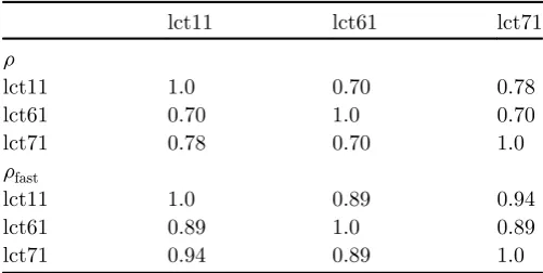
The impact of the method was also tested on a set of thermal criticality benchmarks, lct11, lct61, and lct71. These are low enriched U235, compound and thermal systems (with water) and theirkeffresponses to the ND are
expected to be highly correlated. From the ICSBEP DICE [13] tool the cross-sensitivity between the benchmarks are all quoted to be above 0.9. The benchmarks were all taken from the criticality handbook [14], and the simulations were performed using MCNP. In this case, TENDL2014 U235 [6] data were varied using 1000 randomfiles. Thesstat
was around 250 pcm for the simulations. In Table 1 the results fromrfastare compared to the results for usingr. As
anticipated, higher, and more expected, correlations are obtained using therfast.
The method was also tested for mct011. Here the criteria sstat<0.5s was not met, and unrealistic results
were obtained.
4 Discussion
Is the use of the rfast coefficient important? What is
actually used in error propagation or adjustment is the covariance matrix and not the correlation matrix, and in this sense, the bias in the correlation matrix is of less importance. However, the bias in the correlation matrix clearly affects our interpretation of the results as illustrated in reference [12]. Furthermore, in many cases, a lot of CPU time may be spent to obtain an unbiasedr [10], which can be reduced dramatically ifrfastis used. In
some cases, the correlation itself is used to judge the similarity between benchmarks and applications [11], and in these cases, a good judgment of the correlation is clearly important.
4.1 On cov(xstat,ystat)
An assumption of setting cov(xstat, ystat) to zero is
completely unproblematic in the case of different bench-marks since here the statistical processes of the simulations are completely independent. The authors believe that cov(xstat,ystat), should also be small in the case of [12] data,
and hence the assumption to be reasonable. Ideally, this should be tested by repeating the simulations with constant ND and, e.g., 300 simulations with different seeds; hence the resulting covariances would only stem from the statistics. This has been outside the scope of this study. In some cases, cov(xstat,ystat), can be assumed to be
strong, e.g., for dependent reactor parameters. This has not been investigated in this study.
5 Conclusion
This paper presents a new correlation coefficient,rfast, that
should be considered when investigating correlations between MC code output parameters, obtained by random sampling. In these cases, the Pearson correlation coeffi -cient,r, normally underestimates the correlation andrfast
addresses this issue. The paper presents theoretical arguments for the use ofrfastby its derivation. In addition,
a synthetic data study supports the use of the method. The paper also presents two real cases where the method is used. In these cases, it is harder to draw unambiguous conclusions since the true correlation is unknown. Howev-er, the two studies indicate that the usualrunderestimates the correlation. The presented method is a natural continuation of the fast TMC method presented in reference [5].
The method is tested for ND error propagation when using the neutron transport code MCNP. However, it should be relevant for any type of input parameter variation in any type of MC code.
Author contribution statement
All the authors have contributed to the scientific content of the paper and approved thefinal manuscript.
References
1. O. Buss, A. Hoefer, J.C. Neuber, in Nuduna: Towards a Complete Nuclear Data Uncertainty Estimation for Critical-ity Safety Applications International, Conference on Nuclear
Criticality 2011, Edinburgh (2011)
2. T. Zhu, A. Vasiliev, H. Ferroukhi, A. Pautz, Ann. Nucl. Energy75, 713 (2015)
3. L. Fiorito et al., Ann. Nucl. Energy101, 359 (2017) 4. A.J. Koning, D. Rochman, Nucl. Data Sheets 113, 2841
(2012)
5. D. Rochman, Nucl. Sci. Eng.177, 337 (2014)
6. A.J. Koning, D. Rochman et al., TALYS-Based Evaluated Nuclear Data Library,https://tendl.web.psi.ch/tendl_2015/ tendl2015.html.
Table 1. Correlation coefficients (keffresponses to nuclear
data) between lct11, lct61 and lct 71.
lct11 lct61 lct71
r
lct11 1.0 0.70 0.78
lct61 0.70 1.0 0.70
lct71 0.78 0.70 1.0
rfast
lct11 1.0 0.89 0.94
lct61 0.89 1.0 0.89
lct71 0.94 0.89 1.0
7. P. Helgesson, H. Sjöstrand, D. Rochman, Nucl. Data Sheets
145, 1 (2017)
8. O. Iwamoto, T. Nakagawa, S. Chiba, J. Kor. Phys. Soc.59, 1224 (2011)
9. D. Rochman et al., EPJ Nuclear Sci. Technol.4, 7 (2018) 10. E. Alhassan et al., Ann. Nucl. Energy75, 26 (2015)
11. E. Alhassan et al., Ann. Nucl. Energy96, 26 (2016) 12. N.L. Asquith, S.C. van der Marck, in 16th International
Symposium of Reactor Dosimetry (ISRD16)(2017)
13.https://www.oecd-nea.org/science/wpncs/icsbep/dice.html
14.https://www.oecd-nea.org/science/wpncs/icsbep/hand book.html