Hybrid projected subgradient-proximal algorithms for solving split equilibrium problems and split common fixed point problems of nonexpansive mappings in Hilbert spaces

R E S E A R C H

Open Access

Hybrid projected subgradient-proximal

algorithms for solving split equilibrium

problems and split common fixed point

problems of nonexpansive mappings in

Hilbert spaces

Anteneh Getachew Gebrie

_{and Rabian Wangkeeree}

*_{Correspondence:}

[email protected]

1_{Department of Mathematics,}

Faculty of Science, Naresuan University, Phitsanulok, Thailand

2_{Research Center for Academic}

Excellence in Mathematics, Naresuan University, Phitsanulok, Thailand

Abstract

In this paper, we propose two strongly convergent algorithms which combines diagonal subgradient method, projection method and proximal method to solve split equilibrium problems and split common fixed point problems of nonexpansive mappings in a real Hilbert space: fixed point set constrained split equilibrium problems (FPSCSEPs) in real Hilbert spaces. The computations of first algorthim requires prior knowledge of operator norm. To estimate the norm of an operator is not always easy, and if it is not easy to estimate the norm of an operator, we purpose another iterative algorithm with a way of selecting the step-sizes such that the implementation of the algorithm does not need any prior information as regards the operator norm. The strong convergence properties of the algorithms are established under mild assumptions on equilibrium bifunctions. We also report some

applications and numerical results to compare and illustrate the convergence of the proposed algorithms.

Keywords: nonexpansive mappings; common fixed point problem; equilibrium problem; split equilibrium problem; monotone bifunction; pseudomonotone bifunction; diagonal subgradient method; projected subgradient-proximal algorithm

1 Introduction

In 1994 Censor and Elfving [1] introduced a notion of the split feasibility problem, which is to find an element of a closed convex subset of the Euclidean space whose image un-der a linear operator is an element of another closed convex subset of a Euclidean space. Then, in 2009 Censor and Segal [2] introduced the split common fixed point problem (SCFPP) where split feasibility problem becomes a special case of SCFPP. Many convex optimization problems in a Hilbert space can be written in the form of SCFPP and SCFPPs have played an import role in the study of several unrelated problems arising in physics, finance, economics, network analysis, elasticity, optimization, water resources, medical images, structural analysis, image analysis and several other real-world applications (see,

e.g., [3, 4]). As they have a wide range of applications SCFPPs have emerged as an inter-esting and fascinating research area of mathematics.

Letbe a nonempty closed convex subset of a real Hilbert space H equipped with the inner product·,·and with the corresponding norm · and letU:→be an operator. We denote byFixU={x∈:Ux=x}the subset of fixed points ofU. We say thatUis nonexpansive ifU(x) –U(y) ≤ x–y ∀x,y∈.

Throughout the paper, unless otherwise is stated, we assume thatH1 andH2 be two real Hilbert spaces andA:H1→H2be a nonzero bounded linear operator. SupposeCbe nonempty closed convex subset ofH1andT:C→Cbe nonexpansive operator, andD be nonempty closed convex subset ofH2andV:D→Dbe nonexpansive operator. Given two bifunctionsf :C×C→Randg:D×D→R. The notationEP(f,C) represents the following equilibrium problem:find x∗∈C such that f(x∗,y)≥0∀y∈C, andSEP(f,C) represents its solution set. Many problems in physics, optimization, and economics can be reduced to find the solution of equilibrum problemEP(f,C); see,e.g., [5]. In 1997, Com-bettes and Hirstoaga [6] introduced an iterative scheme of finding the solution ofEP(f,C) under the assumption thatSEP(f,C) is nonempty. Later on, many iterative algorithms are considered to find the element ofFixT∩SEP(f,C); see [7–10]. In 2013, Kazmi and Rizvi [11] considered a split equilibrium problem (SEP):

findx∗∈H1such that ⎧ ⎪ ⎪ ⎪ ⎪ ⎪ ⎨ ⎪ ⎪ ⎪ ⎪ ⎪ ⎩

x∗∈C,

f(x∗,y)≥0, ∀y∈C,

u∗=Ax∗∈D,

g(u∗,u)≥0, ∀u∈D.

They introduced the iterative scheme which converges strongly to a common solution of the split equilibrium problem, the variational inequality problem and the fixed point prob-lem for a nonexpansive mapping. Many researchers have also been proposed algorithms for finding solution point of SEP; see, for example, [12–14] and the references therein. Hieu [14] proposed an algorithm for solving SEP which combines three methods includ-ing the projection method, the proximal method and the diagonal subgradient method. Recently, Dinh, Son, and Anh [15] considered the following fixed point set-constrained split equilibrium problems (FPSCSEPs):

findx∗∈Csuch that ⎧ ⎪ ⎪ ⎪ ⎪ ⎪ ⎨ ⎪ ⎪ ⎪ ⎪ ⎪ ⎩

x∗∈FixT,

f(x∗,y)≥0, ∀y∈C,

u∗=Ax∗∈FixV,

g(u∗,u)≥0, ∀u∈D.

(1)

LetSFPSCSEP(f,C,T;g,D,V) or simplySdenotes the solution set of FPSCSEP (1). The problem (1) includes two fixed point set-constrained equilibrium problems (FPSCEPs). Consider the following fixed point set-constrained equilibrium problem (FPSCEP(f,

C,T)):

findx∗∈Csuch that ⎧ ⎨ ⎩

x∗∈FixT,

and letSFPSCEP(f,C,T) or simplyS1 denotes its solution set. Similarly, letFPSCEP(g,

D,V) denote the fixed point set-constrained equilibrium problem

findu∗∈Dsuch that ⎧ ⎨ ⎩

u∗∈FixV,

g(u∗,u)≥0, ∀u∈D,

(3)

andSFPSCEP(g,D,V) or simplyS2denotes its solution set. Therefore, from (1), (2), and (3) we haveS={x∗∈S1:Ax∗∈S2}. Moreover,S1={x∗∈C:x∗∈SEP(f,C)∩FixT}. Sim-ilarly,S2={u∗∈D:u∗∈SEP(g,D)∩FixV}. In [15], Dinh, Son, and Anh proposed the extragradient algorithms for finding a solution of the problem (FPSCSEP). Under certain conditions on parameters, the proposed iteration sequences are proved to be weakly and strongly convergent to a solution of (FPSCSEP). Furthermore, Dinh, Son, Jiao and Kim [16] proposed the linesearch algorithm which combines the extragradient method incor-porated with the Armijo linesearch rule for solving the problem (FPSCSEP) in real Hilbert spaces under the assumptions that the first bifunction is pseudomonotone with respect to its solution set, the second bifunction is monotone, and fixed point mappings are non-expansive. For obtaining a strong convergence result, they combined the proposed algo-rithm with hybrid cutting technique. The main advantages of the two mentioned extra-gradient methods are that they can be worked with pseudomonotone bifunctions and also the subproblems can be numerically solved more easily than subproblems in the proximal method. However, the problems of solving strongly convex optimization subproblems and of finding shrinking projections in [15, 16] is expensive excepts special cases when the fea-sible set has a simple structure.

In this paper, we propose two strongly convergent algorithms for finding a solution of the problem (FPSCSEP). In the first algorithm, two projections on feasible set and a projected subgradient step followed by a proximal step is need to be computed per each iteration. In the second algorithm, we propose a modification of the first algorithm where the second projection is performed on feasible set while the first projection over C is replaced by a projection onto a tangent plane to C in order to reduce the number of optimization sub-problems to be solved. Moreover, in the second algorithm, a way of selecting an adaptive step-size in the second projection has allowed us to avoid the prior knowledge of operator norm. Comparing with the algorithms in [15, 16], the proposed algorithms has a simple structure, and the metric projection, in general, is simpler than solving strongly convex optimization subproblems on a same feasible set and finding shrinking projections.

The paper is organized as follows. In the next section we describe the properties and lemmas which will be used in the proof for the convergence of the proposed algorithms. The algorithms and the convergence analysis of the algorithms is presented in the third section. Finally, in the last section we will see applications supported by an example and numerical results.

2 Preliminary

To investigate the convergence of our proposed algorithm, in this section we will introduce notations, and recall properties and technical lemmas which will be used in the sequel. We writexnxto indicate that the sequence{xn}converges weakly toxasn→ ∞, and

Letbe a subset of a real Hilbert spaceHandf :×→Rbe a bifunction. Thenf

is said to be

(i) strongly monotoneon, if there isM> 0(shortlyM-strongly monotone on) iff

f(x,y) +f(y,x)≤–My–x2, ∀x,y∈;

(ii) monotoneoniff

f(x,y) +f(y,x)≤0, ∀x,y∈;

(iii) pseudomonotoneonwith respect tox∈iff

f(x,y)≥0 implies f(y,x)≤0, ∀y∈.

We say thatf is pseudomonotone onwith respect to⊂if it is pseudomonotone onwith respect to everyx∈. When=,fis called pseudomonotone on. Clearly, (i)⇒(ii)⇒(iii) for everyx∈.

Definition 2.1 Letbe a nonempty closed convex subset of a real Hilbert spaceH. The metric projection onis a mappingP:H→defined by

P(x) =arg miny–x:y∈.

Properties Letbe a nonempty closed convex subset of a real Hilbert spaceHand letP is a metric projection on. Sinceis nonempty, closed and convex,P(x) exists and is unique. From the definition ofP, it is easy to show thatPhas the following characteristic properties.

(i) For ally∈,

P(x) –x≤ x–y.

(ii) For allx,y∈,

P(x) –P(y)2≤ P(x) –P(y),x–y, ∀x,y∈H.

(iii) For allx∈,y∈H,

x–P(y)2+P(y) –y2≤ x–y2.

(iv) z=P(x)if and only ifx–z,y–z ≤0,∀y∈.

Definition 2.2 LetHbe a Hilbert space andf:×→Rbe a bifunction wheref(x,·) is convex function for eachxin. Then for≥0 the-subdifferential (-diagonal subd-ifferential) off atx, denoted by∂f(x,·)(x) or∂f(x,x), is given by

∂f(x,·)(x) =

Lemma 2.1 Givenλ∈[0, 1],x,y∈H where H is Hilbert space.Then

_{λx+ (1 –}λ)y2=λx2+ (1 –λ)y2–λ(1 –λ)x–y2.

Lemma 2.2(Opial’s condition) For any sequence{xk_{}in the Hilbert space H with x}k_x,

the inequality

lim inf

k→+∞

xk–x<lim inf

k→+∞

xk–y

holds for each y∈H with y=x.

The next lemma will be a useful tool to obtain the boundedness of the sequences gen-erated by the algorithms and also to obtain the convergence of the whole sequence to the solution.

Lemma 2.3 If{ak}∞k=0and{bk}∞k=0are two nonnegative real sequences such that

ak+1≤ak+bk, ∀k≥0

with∞_k=0bk<∞,then the sequence{ak}∞_k=0converges.

Lemma 2.4 Letbe closed and convex subset of a Hilbert space H.If U:→is non-expansive,thenFixU is closed and convex.

Now, we assume that the bifunctions g:D×D→Randf :C×C→Rsatisfy the following assumptions, Condition A and Condition B, respectively.

Condition A

(A1) g(u,u) = 0, for allu∈D.

(A2) gis monotone onD,i.e.,g(u,v) +g(v,u)≤0, for allu,v∈D. (A3) For eachu,v,w∈D,

lim sup

α↓0

gαw+ (1 –α)u,v≤g(u,v).

(A4) g(u,·)is convex and lower semicontinuous onDfor eachu∈D.

Condition B

(B1) f(x,x) = 0for allx∈C.

(B2) f is pseudomonotone onCwith respect tox∈SEP(f,C),i.e., ifx∈SEP(f,C)then

f(x,y)≥0impliesf(y,x)≤0,∀y∈C.

(B3) f satisfies the following condition, called the strict paramonotonicity property:

x∈SEP(f,C),y∈C, f(y,x) = 0⇒y∈SEP(f,C).

(B4) f is jointly weakly upper semicontinuous onC×Cin the sense that, ifx,y∈Cand {xk},{yk} ⊂Cconverge weakly toxandy, respectively, thenf(xk,yk)→f(x,y)as

(B5) f(x,·)is convex, lower semicontinuous and subdifferentiable onC, for allx∈C. (B6) If{xk_{}is bounded sequence inCand}

k→0, then the sequence{wk}with

wk_∈∂ kf(x

k_,·)(xk_{)is bounded.}

The following three results are from equilibrium programming in Hilbert spaces.

Lemma 2.5([17, Lemma 2.12]) Let g satisfies ConditionA.Then,for each r> 0and u∈H2,

there exists w∈D such that

g(w,v) +1

rv–w,w–u ≥0, ∀v∈D.

Lemma 2.6([17, Lemma 2.12]) Let g satisfy ConditionA.Then,for each r> 0and u∈H2,

define a mapping(called the resolvent of g),given by

Tg r(u) =

w∈D:g(w,v) +1

rv–w,w–u ≥0,∀v∈D

.

Then the following holds: (i) Trg is single-valued;

(ii) Trg is a firmly nonexpansive,i.e.,for allu,v∈H,

T_rg(u) –T_rg(v)2≤ T_rg(u) –T_rg(v),u–v;

(iii) Fix(Trg) =SEP(g,D),whereFix(Trg)is the fixed point set ofTrg; (iv) SEP(g,D)is closed and convex.

Lemma 2.7 ([17, Lemma 2.12]) For r,s> 0 and u,v∈H2. Under the assumptions of Lemma2.6,then

Tg

r(u) –Tsg(v)≤ u–v+ |s–r|

s T

g s(v) –v

3 Main result

In this section, we propose two strongly convergent algorithms for solving FPSCSEPs (1) which combines three methods including the projection method, the proximal method and the diagonal subgradient method.

3.1 Projected subgradient-proximal algorithm

Algorithm 3.1

Initialization: Choosex0∈C. Take{ρk},{βk},{k},{rk},{δk}and{μk}such that

ρk≥ρ> 0, βk≥0, k≥0, rk≥r> 0, 0 <a<δk<b< 1,

0 <c≤μk≤b< 1 A2,

∞

k=0

βk

ρk = +∞,

∞

k=0

βkk

ρk < +∞,

∞

k=0

β_k2< +∞.

Step 1: Takewk_∈H

Step 2: Calculate

αk=

βk

ηk

, ηk=max

ρk,wk

and

yk=PC

xk–αkwk

.

Step 3: Evaluate

tk=δkxk+ (1 –δk)T

yk.

Step 4: Evaluate

uk=T_rg_kAtk.

Step 5: Evaluate

xk+1=PC

tk+μkA∗

Vuk–Atk.

Step 6: Setk:=k+ 1 and go to Step 1.

Remark 3.1 Sincef(x,·) is a lower semicontinuous convex function andC⊂domf(x,·) for everyx∈C, then thek-diagonal subdifferential∂kf(x

k_,·)(xk_{)=∅for every} k> 0. Moreover,ρk≥ρ> 0. Therefore, each step of the algorithm are well defined, implying that Algorithm 3.1 is well defined.

Remark 3.2 fis pseudomonotone onCwith respect toSEP(f,C), then under Condition B ((B1) and (B4)), the setSEP(f,C) is closed and convex.

Therefore, by Lemma 2.4, Remark 3.2 and by the linearity property of the operatorA

the solution setSof the FPSCSEP is convex and closed. In this paper, the solution setSis assumed to be nonempty.

Lemma 3.1 Let{yk_},{tk_}and{xk_{}be sequences generated by Algorithm3.1.For x}∗_∈S,

tk–x∗2≤xk–x∗2+ 2αk(1 –δk)f

xk,x∗–Lk+ξk,

where

Lk= (1 –δk)xk–yk 2

+δk(1 –δk)T

yk–xk2

and

ξk= 2(1 –δk)

βkk

ρk

Proof Letx∗∈S. Fromyk_=P

C(xk–ηβ_kkwk) andx∗∈Swe have

xk–αkwk–yk,yk–x∗

≥0,

implying that

x∗–yk,xk–yk≤αkwk,x∗–yk

=αkwk,x∗–xk

+αkwk,xk–yk

≤αkwk,x∗–xk

+αkwkxk–yk. (4)

But alsoxk_{∈C. Thus,}

xk–αkwk–yk,yk–xk

≥0,

and this together with (4) gives us

xk–yk,xk–yk=xk–yk2≤αkwk,xk–yk

≤αkwkxk–yk.

That is,

xk–yk≤αkwk.

Thus,

αkwkxk–yk≤

αkwk2=

βkwk

ηk 2

=β_k2

wk

max{ρk,wk} 2

≤β_k2. (5)

Sincexk∈Candwk∈∂kf(x

k_,·)(xk_{) we have}

fxk,x∗+k=f

xk,x∗–fxk,xk+k

≥ wk,x∗–xk. (6)

Using the definitions ofαkandηkwe obtain

αk=

βk

ηk

= βk

max{ρk,wk}≤

βk

ρk

. (7)

From (4)-(7) we have

x∗–yk,xk–yk≤αkf

xk,x∗+βkk

ρk

+β_k2. (8)

But

From (8) and (9) we have

yk–x∗2≤xn–x∗2–xk–yk2+ 2αkf

xk,x∗+ 2βkk

ρk

+ 2β_k2. (10)

Then by definition oftkwe have tk–x∗2=δkxk+ (1 –δk)T

yk–x∗2

=δk

xk–x∗+ (1 –δk)

Tyk–x∗2

=δkxk–x∗2+ (1 –δk)T

yk–x∗2–δk(1 –δk)T

yk–xk2

=δkxk–x∗2+ (1 –δk)T

yk–Tx∗2–δk(1 –δk)T

yk–xk2

≤δkxk–x∗ 2

+ (1 –δk)yk–x∗ 2

–δk(1 –δk)T

yk–xk2,

and this together with (10) we have

_tk_–x∗2_≤δ

kxk–x∗ 2

+ (1 –δk)

xk–x∗2–xk–yk2

+ 2αkf

xk,x∗+ 2βkk

ρk + 2β_k2

–δk(1 –δk)T

yk–xk2.

That is,

tk–x∗2≤xk–x∗2+ 2αk(1 –δk)f

xk,x∗–Lk+ξk,

where

Lk= (1 –δk)xk–yk 2

+δk(1 –δk)T

yk–xk2

and

ξk= 2(1 –δk)

βkk

ρk

+ 2(1 –δk)βk2.

Remark 3.3 Sincex∗∈SEP(C,f) we havef(x∗,x)≥0 for allx∈C, and by pseudomono-tonicity off with respect toSEP(C,f) we havef(x,x∗)≤0 for allx∈C. Thus since the sequence{xk_{}is inCwe havef(x}k_,x∗_{)≤0. Thus, we can also have}

tk–x∗2≤xk–x∗2–Lk+ξk. (11)

Lemma 3.2 Let{yk_},{uk_},and{xk_{}be sequences generated by Algorithm3.1.Let x}∗_∈S. Then

xk+1–x∗2≤xk–x∗2+ 2(1 –δk)αkf

xk,x∗+ξk–Kk,

where

Kk=μk

1 –μkA2V

uk–Atk2+μkuk–Atk2+ (1 –δk)xk–yk2

+δk(1 –δk)T

and

ξk= 2(1 –δk)

βkk

ρk

+ 2(1 –δk)βk2.

Proof Letx∗∈S. By Lemma 2.6, we have

T_rg kAt

k_–Ax∗2 =T_rg

kAt

k_–Tg rkAx

∗2

≤ T_rg_kAtk–T_rg_kAx∗,Atk–Ax∗

= T_rg_kAtk–Ax∗,Atk–Ax∗

=1 2T

g rkAt

k_–Ax∗2

+Atk–Ax∗2–T_rg kAt

k_–Atk2 .

That is,

T_rg kAt

k_–Ax∗2 ≤1

2T g rkAt

k_–Ax∗2

+Atk–Ax∗2–T_rg kAt

k_–Atk2

. (12)

In view of (12), we have

T_rg_kAtk–Ax∗2≤Atk–Ax∗2–T_rg_kAtk–Atk2.

Thus,

Vuk–Ax∗2=VT_rg_kAtk–VAx∗2

=T_rg_kAtk–Ax∗2

≤Atk–Ax∗2–T_rg_kAtk–Atk2, (13)

which gives

Atk–x∗,Vuk–Atk

= Atk–x∗+Vuk–Atk–Vuk+Atk,Vuk–Atk

= Vuk–Ax∗,Vuk–Atk–Vuk–Atk2

=1 2V

uk–Ax∗2+Vuk–Atk2–Atk–Ax∗2–Vuk–Atk2

=1 2V

uk–Ax∗2–Vuk–Atk2–Atk–Ax∗2.

Hence,

Atk–x∗,Vuk–Atk

=1 2V

uk–Ax∗2–Vuk–Atk2–Atk–Ax∗2. (14)

From (13) and (14) we have

Atk–x∗,Vuk–Atk≤–1 2T

g rkAt

Then from (13) and (15) we have

_xk+1_–x∗2

=PC

tk+μkA∗

Vuk–Atk–PC

x∗

≤tk–x∗+μk

Vuk–Atk2

=tk–x∗2+μkA∗

Vuk–Atk2+ 2μktk–x∗,A∗

Vuk–Atk

≤tk–x∗2+μ2_kA∗2Vuk–Atk2+ 2μkA

tk–x∗,Vuk–Atk

≤tk–x∗2+μ2_kA∗2Vuk–Atk2–μkTαgkAt

k_–Atk2

+Vuk–Atk2

=tk–x∗2–μk

1 –μkA2V

uk–Atk2–μkTrgkAt

k_–Atk2

=tk–x∗2–μk

1 –μkA2V

uk–Atk2–μkuk–Atk2

=tk–x∗2–μk

1 –μkA2V

uk–Atk2–μkuk–Atk 2

.

That is,

xk+1–x∗2≤tk–x∗2–μk

1 –μkA2V

uk–Atk2–μkuk–Atk 2

. (16)

Therefore, from Lemma 3.1 and from (16) we have

xk+1–x∗2≤xk–x∗2+ 2αk(1 –δk)f

xk,x∗–Lk+ξk

–μk

1 –μkA2V

uk–Atk2–μkuk–Atk 2

. (17)

That is,

xk+1–x∗2≤xk–x∗2+ 2(1 –δk)αkf

xk,x∗+ξk–Kk, (18)

where

Kk=μk

1 –μkA2V

uk–Atk2+μkuk–Atk 2

+ (1 –δk)xk–yk 2

+δk(1 –δk)T

yk_–xk2

and

ξk= 2(1 –δk)

βkk

ρk

+ 2(1 –δk)βk2.

Lemma 3.3 Let{yk},{tk},{uk},and{xk}be sequences generated by Algorithm3.1.Then: (i) Forx∗∈S,the limit of the sequence{xk–x∗2}exists(and{xk}is bounded). (ii) lim sup_k→∞f(xk,x) = 0for allx∈S.

(iii)

lim

k→∞V

uk–Atk= lim

k→∞u

k_–Atk_{= 0,}

lim

k→∞

xk–yk= lim

k→∞

(iv)

lim

k→∞t

k_–xk_{= lim} k→∞T

xk–xk= lim

k→∞V

uk–uk= 0.

Proof (i) Letx∗∈S. Sincef(xk_,x∗_)≤0,K

k≥0, from Lemma 3.2 we can have

xk+1–x∗2≤xk–x∗2+ξk.

Observing thatξk= 2(1 –δk)βk_ρk

k + 2(1 –δk)β

2 k≤2

βkk

ρk + 2β

2

k and using the initialization condition of the parameters we can see that∞_k=0ξk<∞.

Therefore,limk→∞xk–x∗2exists and this implies that the sequence{xk}is bounded.

(ii) From lemma 3.2 we have

Kk+ 2(1 –δk)αk

–fxk_,x∗

≤xk–x∗2–xk+1–x∗2+ξk

=xk–x∗2–xk+1–x∗2+ 2(1 –δk)

βkk

ρk

+ 2(1 –δk)βk2

≤xk–x∗2–xk+1–x∗2+ 2βk

ρk

k+ 2βk2.

Summing up the above inequalities for everyN, we obtain

0≤ N

k=0

Kk+ 2(1 –δk)αk

–fxk,x∗

≤ N

k=0

xk–x∗2–xk+1–x∗2+ 2βk

ρk

k+ 2βk2

.

This will yield

0≤ N

k=0

Kk+ N

k=0

2(1 –δk)αk

–fxk,x∗

≤x0–x∗2–xN+1–x∗2+ 2 N

k=0

βk

ρk

k+ 2 N

k=0

β_k2.

LettingN→+∞, we have

0≤

∞

k=0

Kk+

∞

k=0

2(1 –δk)αk

–fxk,x∗< +∞.

Hence,

∞

k=0

and

∞

k=0

2(1 –δk)αk

–fxk,x∗< +∞.

Since the sequence{xk_{}is bounded by Condition B(B6) the sequence{w}k_{}is also bounded.} Thus, there is a real numberw≥ρsuch thatwk _{≤w. Thus,}

αk=

βk

ηk

= βk

max{ρk,wk}

= βk

ρkmax{1,w

k

ρk }

≥βkρ

ρkw

. (20)

Noting

0≤2(1 –b)

∞ k=0 αk

–fxk,x∗≤ ∞

k=0

2(1 –δk)αk

–fxk,x∗< +∞,

we have

0≤2(1 –b)

∞ k=0 αk

–fxk,x∗< +∞. (21)

From (20) and (21) we have

0≤2(1 –b)

∞

k=0

βkρ

ρkw

–fxk,x∗≤2(1 –b)

∞ k=0 αk

–fxk,x∗< +∞.

That is,

0≤2ρ(1 –b)

w ∞ k=0 βk ρk

–fxk,x∗< +∞.

Since∞_k=0βk

ρk = +∞and –f(x

∗_,xk_{)≤0 we can conclude that}

lim sup

k→∞ f

xk,x= 0

for allx∈S.

(iii) From (19) and since 0 <c≤μk≤b<_A12, 0 <δk< 1 we have

lim

k→∞V

uk–Atk2= lim

k→∞u

k_–Atk2 = lim

k→∞x

k_–yk2 = lim

k→∞T

yk–xk2= 0.

Hence, the result follows.

(iv) The result follows from (iii) and from the following inequalities:

tk–xk≤δkxk+ (1 –δk)T

yk–xk= (1 –δk)xk–T

yk≤xk–Tyk, Txk–xk≤Txk–Tyk+xk–Tyk≤xk–yk+xk–Tyk,

Theorem 3.4 Assume ConditionAand ConditionBare satisfied and let{yk_},{tk_},{uk_},

and{xk_{},be sequences generated by Algorithm3.1.Then the sequences{y}k_},{tk_}and{xk_}

converge strongly to a point p∈S and{uk_{}converge strongly to a point Ap∈S2.Moreover,}

p= lim

k→+∞PS

xk.

Proof Letx∗∈S. From Lemma 3.3(i) we have seen that the sequence{xk_{} is bounded.} There exists a subsequence {xkj} _of {_xk} _{such that x}kj _{pas j}→₊∞_{, where p}∈_C

and

lim sup

j→+∞

fxkj_,x∗_{= lim}

i→+∞f

xki_,x∗_.

But by the weakly upper semicontinuity off(·,x∗) and by Lemma 3.3(ii) we have

fp,x∗≥lim sup

j→+∞

fxkj_,x∗_{= lim}

i→+∞f

xki_,x∗_{=lim sup}

k→+∞ f

xk,x∗= 0.

Sincex∗∈Sandp∈Cwe havef(x∗,p)≥0. Asf is pseudomonotone we havef(p,x∗)≤0. Thus, this together with the above fact givesf(x∗,p) = 0. Hence, by Condition B(B3) we havep∈SEP(f,C).

Since

ykj_{,h= y}kj_–xkj_{,h+ x}kj_,h, ∀_h∈_H1,

and usinglimk→+∞xk–yk= 0 from Lemma 3.3 we haveykjpasj→+∞. Therefore,

Aykj_Apasj→+∞. Similarly, we can have_tkj_pasj→+∞_{and henceAt}kj_Apas j→+∞.

Assumep∈/FixT, that is,T(p)=p. Thus, using Opial’s condition and Lemma 3.3

lim inf

j→+∞x

kj_{–p<lim inf}

j→+∞x

kj_–T(p)

=lim inf

j→+∞x

kj_–Txkj_+Txkj_–T(p)

≤lim inf

j→+∞

_xkj_–Txkj_+Txkj_–T(p)

=lim inf

j→+∞

Txkj_–T(p)

≤lim inf

j→+∞

xkj_–p,

which is a contradiction. Hence, it must be the case thatp∈FixT. Hence,

p∈S1. (22)

Sincelimk→+∞uk–Atk= 0 and

we have ukj _{Ap asj}→+∞. Assume _Ap∈_{/ FixV. Thus, using Opial’s condition and}

Lemma 3.2

lim inf

j→+∞

ukj_{–Ap<lim inf}

j→+∞

ukj_–V(Ap)

=lim inf

j→+∞u

kj_–Vukj_+Vukj_–V(Ap)

≤lim inf

j→+∞u

kj_–Vukj_+Vukj_–V(Ap)

=lim inf

j→+∞

Vukj_–V(Ap)

=lim inf

j→+∞

ukj_–Ap,

which is a contradiction. Hence, it must be the case thatAp∈FixV. Letr> 0. Assume

Ap∈/ Fix(Trg). Thus,Trg(Ap)=Ap. Thus, using Opial’s condition, Lemma 3.2, Lemma 3.3 we obtain the following:

lim inf

j→+∞At

kj_{–Ap<lim inf}

j→+∞At

kj_–Tg

r(Ap)

=lim inf

j→+∞At

kj_–ukj_+ukj_–Tg

r(Ap)

≤lim inf

j→+∞

Atkj_–ukj_+ukj_–Tg

r(Ap)

=lim inf

j→+∞

ukj_–Tg

r(Ap)

=lim inf

j→+∞T

g r_kj

Atkj_–Tg

r(Ap)

≤lim inf

j→+∞

Atkj_–Ap+|rkj–r| rkj

T_rgAtkj_–Atkj

=lim inf

j→+∞

Atkj_–Ap+|rkj–r| rkj

ukj_–Atkj

=lim inf

j→+∞

Atkj_–Ap,

which is a contradiction. Hence, it must be the case thatAp∈Fix(Trg). By Lemma 2.6(iii) we haveAp∈SEP(g,D). Therefore,

Ap∈S2. (23)

Therefore, from (22) and (23) we havep∈S. That is,p∈Sandpis a weak cluster point of the sequence{xk_{}. By Lemma 3.3{x}k_–p2_{}converges. Hence, we conclude that the} sequence{xk}strongly converges top. As a result of this it is easy to see thattk→pand

yk→pasj→+∞. Moreover,Ayk→Ap,Atk→Ap, andAxk→Ap. From

we haveuk_{→Ap. We will end the proof by showingp=lim}

k→+∞PS(xk). From Lemma 3.2 we have

xk+1–x∗2≤xk–x∗2+ξk, ∀x∗∈S. (24)

Letzk=PS(xk). SincePS(xk)∈Swe have

xk+1–zk2≤xk–zk2+ξk. (25)

But by property of metric projection we have

_xk+1_–zk+12_≤xk+1_–x∗2_{, ∀x}∗_∈S.

Thus,

xk+1–zk+12≤xk+1–zk2. (26)

From (25) and (26) we have

xk+1–zk+12≤xk–zk2+ξk.

Since∞_k=0ξk<∞, by Lemma 2.3 we see thatlimk→+∞xk–zk2exists. Using the

defini-tion of a metric projecdefini-tion we can have

_PS

xn–PS

xm2+xm–PS

xm2≤xm–PS

xn2. (27)

Letm≥n. Then using (24) and (27) we have

zn–zm2=PS

xn–PS

xm2

≤xm–PS

xn2–xm–PS

xm2

=xm–zn2–xm–zm2

≤xm–1–zn2+ξm–1–xm–zm 2

≤xn–zn2+ m–1

i=n

ξm–1–xm–zm 2

.

As a result of∞_k=0ξk<∞andlimk→+∞xk–zk2exists if we letm,n→+∞we can see thatzn–zm2→0. This implies the sequence{zk}is a Cauchy sequence and hence it converges to some pointzinS. Sincezk_=P

S(xk) we have

xk–zk,x∗–zk≤0, ∀x∗∈S.

Thus

Thus,

z–p2=p–z,p–z= lim

k→+∞x

k_–zk_,p–zk_≤0.

Hence,p=zandlimk→+∞PS(xk) =p.

Let Id represents identity operator. Then, if T= Id and V = Id, then FPSCSEP (1) is reduced to SEP. Hence, Algorithm 3.1 can be rewritten as follows.

Algorithm 3.1B

Initialization: Choosex0∈C. Take{ρk},{βk},{k},{rk},{δk}and{μk}such that

ρk≥ρ> 0, βk≥0, k≥0, rk≥r> 0, 0 <a<δk<b< 1,

0 <c≤μk≤b< 1 A2,

∞

k=0

βk

ρk = +∞,

∞

k=0

βkk

ρk < +∞,

∞

k=0

β_k2< +∞.

Step 1: Takewk∈H1such thatwk∈∂kf(x

k_,·)(xk_).

Step 2: Calculate

αk=

βk

ηk

, ηk=max

ρk,wk

and

yk=PC

xk–αkwk

.

Step 3: Evaluate

tk=δkxk+ (1 –δk)yk.

Step 4: Evaluate

uk=T_rg_kAtk.

Step 5: Evaluate

xk+1=PC

tk+μkA∗

uk–Atk.

Step 6: Setk:=k+ 1 and go to Step 1.

The following corollary is an immediate consequence of Theorem 3.4.

Corollary 3.5 Let H1 and H2be two real Hilbert spaces and A:H1→H2be a nonzero

ConditionAand ConditionBare satisfied and let{yk_},{tk_},{uk_},and{xk_{},be sequences}

generated by Algorithm3.1B.If S={x∗∈SEP(f,C) :Ax∗∈SEP(g,D)} =∅,then sequences

{yk_},{tk_}and{xk_{}converge strongly to a point p∈S and{u}k_{}converges strongly to a point}

Ap∈SEP(g,D).

3.2 Modified projected subgradient-proximal algorithm

The computation of Algorithm 3.1 involves the evaluation of two projections on the feasi-ble setCand the estimated value of operator normA. It is not an easy task to calculate or at least to estimate the operator normA. Based on Algorithm 3.1, we propose an algo-rithm with a way of selecting the step-sizes such that its implementation does not need any prior information as regards the operator norm, and the algorithm involves only one projection on the feasible setC.

For any α > 0 define hα(x) = 1₂VTαgA(x) –A(x)2 for all x∈ H1, and so ∇hα(x) =

A∗(VTαgA(x) –A(x)).

Algorithm 3.2

Initialization: Choosex0_{∈C. Take{ρ}

k},{βk},{k},{rk},{δk}and{ηk}such that

ρk≥ρ> 0, βk≥0, k≥0, rk=r> 0, 0 <a<δk<b< 1,

0 <η≤ηk≤4 –η,

∞

k=0

βk

ρk = +∞,

∞

k=0

βkk

ρk < +∞,

∞

k=0

β_k2< +∞.

Step 1: Findwk∈H1such thatwk∈∂kf(x

k_,·)(xk_).

Step 2: Evaluateyk_=P

Tk(xk–αkwk) whereαk=

βk

ηk,ηk:=max{ρk,w

k_{}, andT}

0=C,Tk= {z∈H1:tk–1+μk–1∇hr(tk–1) –xk,z–xk ≤0}fork= 1, 2, 3, . . . .

Step 3: Evaluatetk_=δ

kxk+ (1 –δk)T(yk).

Step 4: Evaluateuk=Trg(Atk).

Step 5: Evaluate

xk+1=PC

tk+μk∇hr

tk,

where

μk= ⎧ ⎨ ⎩

0, if∇hr(tk) = 0, ηkhr(tk)

∇hr(tk)2, otherwise.

Step 6: Setk=k+ 1 and go to Step 1.

Remark 3.4 By definition ofTk, we see thatTk is either half-space or the whole space

H1. Therefore, for eachk,Tkis closed and convex set, and the computation of projection

yk=PTk(x

k_–α

kwk) in Step 2 of Algorithm 3.2 is explicit and easier than the computation of projectionyk_=P

Lemma 3.6 Let{yk_},{tk_}and{xk_{}be sequences generated by Algorithm3.2.} (i) C⊂Tkfor allk≥0.

(ii) Forx∗∈S,

tk–x∗2≤xk–x∗2+ 2αk(1 –δk)f

xk,x∗–Lk+ξk,

where

Lk= (1 –δk)xk–yk 2

+δk(1 –δk)T

yk–xk2

and

ξk= 2(1 –δk)

βkk

ρk

+ 2(1 –δk)βk2.

Proof (i) Fromxk_=P

C(tk–1+μk–1∇hr(tk–1)) and by property of metric projection we have

tk–1+μk–1∇hr

tk–1–xk,z–xk, ∀z∈C,

which together with the definition ofTkimplies thatC⊂Tk. (ii) Letx∗∈S. Fromyk_=P

Tk(x

k_–βk

ηkw

k_{) andx}∗_,xk_∈C⊂T

kwe have

xk–αkwk–yk,yk–x∗

≥0.

Then, with a similar proof as for Lemma 3.1 we have

tk–x∗2≤xk–x∗2+ 2αk(1 –δk)f

xk,x∗–Lk+θk,

where

Lk= (1 –δk)xk–yk2+δk(1 –δk)T

yk–xk2

and

ξk= 2(1 –δk)

βkk

ρk

+ 2(1 –δk)βk2.

Lemma 3.7 Let{yk_},{uk_},and{xk_{}be sequences generated by Algorithm3.2.For x}∗_∈S

xk+1–x∗2≤xk–x∗2+ 2(1 –δk)αkf

xk,x∗+ξk–Kk–ωk,

where

Kk= (1 –δk)xk–yk 2

+δk(1 –δk)T

yk–xk2–T_rg_kAtk–Atk2,

ξk= 2(1 –δk)

βkk

ρk

and

ωk= ⎧ ⎨ ⎩

0, if∇hr(tk) = 0,

ηk(4 –ηk) hr(t

k₎

∇hr(tk)2, otherwise.

Proof Letx∗∈S. By Lemma 2.6,

T_rgAtk–Ax∗2=T_rgAtk–T_rgAx∗2

≤ T_rgAtk–T_rgAx∗,Atk–Ax∗

= T_rgAtk–Ax∗,Atk–Ax∗

=1 2T

g

rAtk–Ax∗ 2

+Atk_–Ax∗2_–Tg

rAtk–Atk 2

.

That is,

T_rgAtk–Ax∗2≤1

2T g

rAtk–Ax∗ 2

+Atk–Ax∗2–T_rgAtk–Atk2. (28)

In view at (28) we get

_Tg

rAtk–Ax∗ 2

≤Atk–Ax∗2–T_rgAtk–Atk2.

Hence,

Vuk–Ax∗2≤T_rgAtk–Ax∗2≤Atk–Ax∗2–T_rgAtk–Atk2. (29)

Using (29) we have

tk–x∗,∇hr

tk

= tk–x∗,A∗Vuk–Atk

= Atk–x∗,Vuk–Atk

= Atk–x∗+Vuk–Atk–Vuk+Atk,Vuk–Atk

= Vuk–Ax∗,Vuk–Atk–Vuk–Atk2

=1 2V

uk–Ax∗2+Vuk–Atk2–Atk–Ax∗2–Vuk–Atk2

=1 2V

uk–Ax∗2–Vuk–Atk2–Atk–Ax∗2

≤–1 2T

g

rAtk–Atk 2

+Vuk–Atk2

= –1 2T

g

rAtk–Atk 2

+ 2hr

tk.

That is,

tk–x∗,∇hr

tk≤–1 2u

k_–Atk2_{+ 2h} r

By Lemma 2.6 and (30), we have

xk+1–x∗2=PC

tk+μk∇hr

tk–PC

x∗2

≤tk+μk∇hr

tk–x∗2

=tk–x∗2+μ2_k∇hr

tk2– 2μk∇hr

tk,tk–x∗

≤tk–x∗2+μk∇hr

tk2– 4μkhr

tk–uk–Atk2

=tk–x∗2–uk–Atk2–4μkhr

tk–μk∇hr

tk2.

That is,

xk+1–x∗2≤tk–x∗2–uk–Atk2–4μkhr

tk–μk∇hr

tk2. (31)

Therefore, using (31) and Lemma 3.6, we have

xk+1–x∗2≤xk–x∗2+ 2(1 –δk)αkf

xk,x∗+ξk–Kk–ωk,

where

Kk= (1 –δk)xk–yk2+δk(1 –δk)T

yk–xk2–uk–Atk2,

ξk= 2(1 –δk)

βkk

ρk

+ 2(1 –δk)βk2,

and

ωk= 4μkhr

tk–μk∇hr

tk2.

Note that by the definition ofμkwe have

ωk= ⎧ ⎨ ⎩

0, if∇hr(tk) = 0,

ηk(4 –ηk) hr(t

k₎

∇hr(tk₎2, otherwise.

Lemma 3.8 Let{yk_},{tk_},{uk_},and{xk_{}be sequences generated by Algorithm3.2.Then:} (i) Forx∗∈S,the limit of the sequence{xk_–x∗2_{}exists(and{x}k_{}is bounded).} (ii) lim sup_k→∞f(xk_{,x) = 0for allx∈S.}

(iii)

lim

k→∞u

k_–Atk_{= lim} k→∞x

k_–yk_{= lim} k→∞T

yk–xk= 0,

lim

k→∞t

k_–xk_{= lim} k→∞T

xk–xk= 0.

(iv)

lim

k→∞hr

tk= lim

k→∞

Proof (i) Letx∗∈S. Sincef(xk_,x∗_)≤0,K

k≥0,ωk≥0 from Lemma 3.2 we can have xk+1–x∗2≤xk–x∗2+ξk.

Therefore, the result follows. (ii) From Lemma 3.7 we can have

ωk+Kk+ 2(1 –δk)αk

–fxk,x∗≤xk–x∗2–xk+1–x∗2+ξk

≤xk–x∗2–xk+1–x∗2+ 2βk

ρk

k+ 2βk2.

Summing up the above inequalities for everyN, we obtain

0≤ N

k=0

ωk+Kk+ 2(1 –δk)αk

–fxk,x∗

≤ N

k=0

xk–x∗2–xk+1–x∗2+ 2βk

ρk

k+ 2βk2

.

This will yield

0≤ N

k=0

ωk+ N

k=0

Kk+ N

k=0

2(1 –δk)αk

–fxk_,x∗

≤x0–x∗2–xN+1–x∗2+ 2 N

k=0

βk

ρk

k+ 2 N

k=0

β_k2.

LettingN→+∞, we have

0≤

∞

k=0

ωk+

∞

k=0

Kk+

∞

k=0

2(1 –δk)αk

–fxk,x∗< +∞.

Hence,

∞

k=0

ωk< +∞,

∞

k=0

Kk< +∞,

∞

k=0

2(1 –δk)αk

–fxk,x∗< +∞. (32)

In the same way as proving Lemma 3.2 the result follows. (iii) From∞_k=0Kk< +∞and 0 <δk< 1 we have

lim

k→∞u

k_–Atk2 = lim

k→∞x

k_–yk2 = lim

k→∞T

yk–xk2= 0.

The remaining result follows from the following inequalities: tk–xk≤δkxk+ (1 –δk)T

yk–xk= (1 –δk)xk–T

yk≤xk–Tyk

and

(iv) From (32) we have∞_k=0[4μkhr(tk) – (μk∇hr(tk))2] < +∞. Without loss of general-ity, we can assume that∇hr(tk)= 0 for allk. Thus,

_∞

k=0[4μkhr(tk) – (μk∇hr(tk))2] < +∞ implies that

∞

k=0

ηk(4 –ηk)

hr(tk) ∇hr(tk)2

< +∞.

Since 0 <η≤ηk≤4 –ηwe have

∞

k=0

hr(tk) ∇hr(tk)2

< +∞.

Sincelimk→∞tk–xk= 0 and{xk}is bounded,{tk}is also bounded. Thus, it follows from the Lipschitz continuity of∇hr(·) that{∇hr(tk)2}is bounded. This together with the last relation implies thatlimk→∞hr(tk) = 0. The inequalityV(uk) –uk ≤(2hr(tk))

1

2 +uk–

Atk_yields

lim

k→∞

Vuk–uk= 0.

Theorem 3.9 Assume ConditionAand ConditionBare satisfied and let{yk},{tk},{uk}, and{xk_{},be sequences generated by Algorithm3.2.Then the sequences{y}k_},{tk_}and{xk_}

converge strongly to a point p∈S and{uk_{}converge strongly to a point Ap∈S2.Moreover,}

p= lim

k→+∞PS

xk.

Proof With consideration of the definition ofhr(tk) the proof remains the same as for

Theorem 3.4.

For any α > 0 define hα(x) = ₂1TαgA(x) –A(x)2 for all x ∈H1, and so ∇hα(x) =

A∗(TαgA(x) –A(x)). SettingT= Id andV= Id, the FPSCSEP (1) is reduced to SEP. Hence, Algorithm 3.2 can be rewritten as follows:

Algorithm 3.2B

Initialization: Choosex0_{∈C. Take{ρ}

k},{βk},{k},{rk},{δk}and{ηk}such that

ρk≥ρ> 0, βk≥0, k≥0, rk=r> 0, 0 <a<δk<b< 1,

0 <η≤ηk≤4 –η,

∞

k=0

βk

ρk = +∞,

∞

k=0

βkk

ρk < +∞,

∞

k=0

β_k2< +∞.

Step 1: Findwk_∈H

1such thatwk∈∂kf(x

k_,·)(xk_).

Step 2: Evaluateyk_=P Tk(x

k_–α

kwk) whereαk=β_ηk

k,ηk:=max{ρk,w

k_}and

Tk= ⎧ ⎨ ⎩

C, ifk= 0,

Step 3: Evaluatetk_=δ

kxk+ (1 –δk)yk.

Step 4: Evaluateuk_=Tg r(Atk).

Step 5: Evaluate

xk+1=PC

tk+μk∇hr

tk,

where

μk= ⎧ ⎨ ⎩

0, if∇hr(tk) = 0, η_khr(tk)

∇hr(tk₎2, otherwise.

Step 6: Setk=k+ 1 and go to Step 1.

The following corollary is an immediate consequence of Theorem 3.9.

Corollary 3.10 Let H1and H2be two real Hilbert spaces and A:H1→H2be a nonzero

bounded linear operator.Suppose C be nonempty closed convex subset of H1,D be nonempty closed convex subset of H2,and f :C×C→Rand g:D×D→Rbe bifunction.Assume ConditionAand ConditionBare satisfied and let{yk_},{tk_},{uk_},and{xk_{},be sequences}

generated by Algorithm3.2B.If S={x∗∈SEP(f,C) :Ax∗∈SEP(g,D)} =∅,then sequences

{yk},{tk}and{xk}converge strongly to a point p∈S and{uk}converges strongly to a point Ap∈SEP(g,D).

4 Application and numerical result

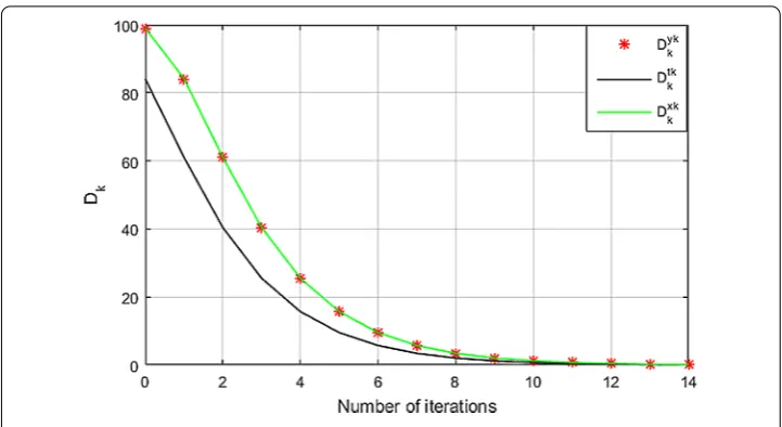
In this section we will see some applications and we perform several numerical exper-iments to illustrate the computational performance of the proposed algorithms (Algo-rithm 3.1 and Algo(Algo-rithm 3.2) and we compare the convergence of one with the other.

LetA:H1→H2 be nonzero bounded linear operator whereH1 andH2 be two real Hilbert spaces, andCandDbe two nonempty closed convex subsets ofH1andH2, re-spectively. Letψ:C→Randφ:D→Rbe functions withψandφare convex and lower semicontinuous, andψ is upper semicontinuous and-subdifferentiable at every point inC. Then the following is an optimization problem:

findx∗∈H1such that ⎧ ⎪ ⎪ ⎪ ⎪ ⎪ ⎨ ⎪ ⎪ ⎪ ⎪ ⎪ ⎩

x∗∈C,

ψ(x∗)≤ψ(y), ∀y∈C,

u∗=Ax∗∈D,

φ(u∗)≤φ(v), ∀v∈D.

(33)

Setf(x,y) =ψ(y) –ψ(x) andg(u,v) =φ(v) –φ(u). Thus,gsatisfies Condition A andf sat-isfies Condition B as a result of the given conditions satisfied byψandφ. Therefore, op-timization problem (33) is SEP which is particular case of FPSCSEP, and Algorithm 3.1B and Algorithm 3.2B solves (33).

Let H be real Hilbert spaces, and C be nonempty closed convex subset of H. Let

multi-objective optimization problem:

minψ(x),φ(x)

s.t.x∈C.

(34)

Therefore, multi-objective optimization problem (34) is equilibrium problem which is also a particular case of FPSCSEP. Next we will see simple case optimization problem and its numerical result as an application. The algorithms are coded in Matlab R2017a (9.2.0.556344) and are operated on MacBook 1.1 GHz Intel Core m3 8 GB 1867 MHz LPDDR3.

Example 4.1 Consider the fixed point constrained optimization problem

findx∗∈Csuch that ⎧ ⎪ ⎪ ⎪ ⎪ ⎪ ⎨ ⎪ ⎪ ⎪ ⎪ ⎪ ⎩

x∗∈FixT,

ψ(x∗)≤ψ(y), ∀y∈C,

u∗=Ax∗∈FixV,

φ(u∗)≤φ(v), ∀v∈D,

where R=H1, R2=H2,A:H1→H2 given byA(x) = (–x₂,x₂),C={x∈R:x≥1},D= {(u1,u2)∈R2:u2–u1≥1},ψ:C→Rgiven byψ(x) = 2x+ 5, andφ:D→Rgiven by

φ(u) =φ(u1,u2) =u2–u1, and the nonexpansive mappingsT:C→Cgiven byT(x) =u+1₂ andV:D→Dgiven byV(u) =V(u1,u2) = (–u2, –u1).

Setf(x,y) =ψ(y) –ψ(x) = 2y– 2xandg(u,v) =φ(v) –φ(u) = (v2–v1) – (u2–u1). It is easy to check thatgandf satisfy Condition A and Condition B, respectively. It is also clear to see thatA∗(u) =A∗(u1,u2) = –1₂u1+1₂u2 andA= 1₂. Hence,FixT ={1},

SEP(f,C) ={1},FixV={(u1,u2)∈D:u2= –u1}, andSEP(g,D) ={(u1,u2)∈D:u2–u1= 1}. Therefore, SFPSCEP(f,C,T) = {1} and SFPSCEP(g,D,V) ={(–1₂,1₂)}. Since A(1) = (–1₂,1₂), we see that the solution set of this problem is singleton setS={p}wherep= 1.

Initialization for Algorithm3.1: Takeρk= 1,k= 0,μk=1₂,rk=₁₀₀₀1 ,βk=log_8k(₊₁₆k+4) and

δk=3

k+1₊₁₀₀

100(3k+1₎.

Initialization for Algorithm3.2: Takeρk= 1,k= 0,ηk= 1,rk=r=₁₀₀₀1 ,βk=log_8k(₊₁₆k+4)and

δk=3

k+1₊₁₀₀

100(3k+1₎.

Note that this choice of parameters satisfies the initialization of each of the algorithms. Choosex0∈C. Letxk,wk,yk,tk,x,yare inR, anduk= (uk₁,u₂k),v= (v1,v2) inR2. For this example Algorithm 3.1 is expressed as an iteration,

⎧ ⎪ ⎪ ⎪ ⎪ ⎪ ⎪ ⎪ ⎪ ⎪ ⎪ ⎪ ⎪ ⎨ ⎪ ⎪ ⎪ ⎪ ⎪ ⎪ ⎪ ⎪ ⎪ ⎪ ⎪ ⎪ ⎩

yk₌ ⎧ ⎨ ⎩

xk_–β

k, ifxk–βk≥0, 1, otherwise,

tk_=δ

kxk+ (1 –δk)y

k₊₁

2 ,

uk_{= (} 1 1000–

1 2t

k_{, –} 1 1000+

1 2t

k_),

xk+1= ⎧ ⎨ ⎩

3tk_–uk 1+uk2

4 , if 3t k_–uk

1+uk2≥4, 1, otherwise,