Multi-sensor Doppler radar for machine tool collision detection

Adv. Radio Sci., 12, 35–41, 2014 www.adv-radio-sci.net/12/35/2014/ doi:10.5194/ars-12-35-2014

© Author(s) 2014. CC Attribution 3.0 License.

Multi-sensor Doppler radar for machine tool collision detection

T. J. Wächter1, U. Siart1, T. F. Eibert1, and S. Bonerz2

1_{Technische Universität München, Lehrstuhl für Hochfrequenztechnik, Arcisstr. 21, 80333 Munich, Germany} 2_{Ott-Jakob Spanntechnik GmbH, Industriestr. 3–7, 87663 Lengenwang, Germany}

Correspondence to: T. J. Wächter ([email protected])

Received: 26 January 2014 – Revised: 11 July 2014 – Accepted: 16 July 2014 – Published: 10 November 2014

Abstract. Machine damage due to tool collisions is a widespread issue in milling production. These collisions are typically caused by human errors. A solution for this problem is proposed based on a low-complexity 24 GHz continuous wave (CW) radar system. The developed monitoring system is able to detect moving objects by evaluating the Doppler shift. It combines incoherent information from several spa-tially distributed Doppler sensors and estimates the distance between an object and the sensors. The specially designed compact prototype contains up to five radar sensor modules and amplifiers yet fits into the limited available space. In this first approach we concentrate on the Doppler-based position-ing of a sposition-ingle movposition-ing target. The recorded signals are pre-processed in order to remove noise and interference from the machinery hall. We conducted and processed system mea-surements with this prototype. The Doppler frequency esti-mation and the object position obtained after signal condi-tioning and processing with the developed algorithm were in good agreement with the reference coordinates provided by the machine’s control unit.

1 Introduction

Collisions within the operating space of machine tools have many different causes. Main causes for collisions during hu-man operation are wrong programming (wrong part, com-pensation or offsets), wrong machine setup (wrong tool, clamping or raw parts) and inattention or faulty operation by the operator himself.

The so called technological collisions concern crashes be-tween tool and work piece only. The second group, the ge-ometric collisions, involves further elements of the machine like the bearings, holder, spindle, axis or the driving shaft.

In the case of tool collisions, tremendous impact forces cause heavy damage to the work piece, the tool and to other elements of the drive train. The results are expensive damage, costs for production downtimes and high rejection rates. The goal is to guarantee high machine availability to maximize efficiency and output.

Up to now, no system is known which reliably provides information in order to avoid collisions with non-moving components and to actively protect the machine components against physical damage. There are some promising sensor based systems that can decouple the inner main motor spin-dle from the outer spinspin-dle stock, hence protecting the compo-nents from mechanical overload to reduce damage to a min-imum. Other methods, without sensors, monitor the current flux through the motor and driving chain and activate when a certain threshold is exceeded. An elaboration on available safety systems can be found in Abele et al. (2012). All of these are reactive systems which are activated after a crash. With these, mitigation of damage is possible, but not their prevention.

Optical systems like laser scanners or (multi-)camera based systems are active observers. The disadvantage of these systems is that they are blinded due to cooling fluid, drizzle, dust and dirt from the milling treatment which pol-lute the lens or the sensor space. So their use is limited to phases where the metal processing is stopped or to other ap-plications with non-cutting manufacture.

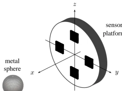
In this paper, the implementation of a prototype for a new possible solution is presented based on an autonomous ac-tive radar sensor safety system which operates in the 24 to 24.25 GHz ISM band. The utilized sensors are commercially available low-cost modules for short-range radar (SRR) ap-plications, containing all front-end parts of a CW radar, including complex down-conversion. Figure 1 shows the prototype concept, here equipped with four modules in a

x y z

metal sphere

sensor platform

Fig. 1. Concept of the toroidal holder with four modules in a sym-metric arrangement and the internal coordinate system. A metal sphere serves as a measurement target.

milling machine tool to provide complete coverage of the

three-dimensional surrounding space.

We designed a toroidal holder with integrated low-noise

amplifiers (LNAs) which allows test scenarios with

differ-ent antenna configurations involving up to five radar

mod-ules with variable radial distance, angle and positions in

x

-direction. Figure 2 shows the implementation with four radar

modules and the corresponding integrated LNAs embedded

in an open test environment. Some important properties of

this additional system and the CW concept are its

indepen-dence from the acting machine tool, robustness against

envi-ronmental influences and reliability due to its simplicity.

Microwave sensorics is more suited for this application

than cameras and optical sensors. This is due to the

su-perior properties of microwaves with the above-mentioned

problems with dirt and moisture in the operating space.

Mi-crowave sensorics is also more suited than acoustical and

ultrasonic sensors. The speed of sound (

300

mm/ms) causes

long signal delays compared to electromagnetic wave

propa-gation.

Operation inside the enclosure of the machine and

process-ing the diverse radar returns from there is one of the

chal-lenges for the signal processing. Multiple reflexions at the

walls at arbitrary distances cause clutter effects and increase

the noise level. Further challenges are the non-stationary

environment, varying shapes and geometries of the milling

tools as well as swarf from treatment in the operating zone.

The system development concentrated on using CW radar

only. This, on the one hand, is due to the robustness of the

technology and the low cost arguments of the electronic

hard-ware. On the other hand, the available space in any machine

tool is limited. This only permits additional components of

small size and low complexity. Furthermore, the large

oper-ating temperature range and the rapid fluctuation of

temper-ature must be dealt with by the equipment to meet the high

Fig. 2. The implemented toroidal sensor platform equipped with four radars and integrated amplifiers embedded in an accessible, maneuverable test environment. Obtained signals are conducted via coaxial lines to the data storage and processing system.

distance information. Also the use of the

24

GHz wideband

technology with

5

GHz bandwidth as in automotive SRR was

ceased as of June 2013 (Strohm et al., 2005). The necessary

bandwidth for a specific range resolution

∆

r

can be derived

from

∆

r

=

c

/

(2∆

f

)

, where

c

is the speed of light and

∆

f

is the absolute bandwidth. With the automotive SRR, a

suffi-cient resolution of

3

cm is achievable if the full bandwidth of

5

GHz is be used.

A second figure of merit is the accuracy

δr

which is

de-fined as (e.g., Skolnik, 1960; Barton, 1964),

δr

=

τ

c

√

2SNR

,

(1)

with the pulse rise time

τ

and the signal-to-noise ratio

SNR

.

Just like the resolution, the accuracy depends on the

band-width which determines

τ

≈

0

.

35

/

∆

f

. Both conditions,

sufficient range resolution and accuracy, cannot be met in the

24

GHz to

24

.

25

GHz ISM-band.

2

Designed Multi-Sensor Doppler Radar Network

From the viewpoint of hardware one of the limiting factors in

this application is the available installation space in the

ma-chine tool. A block diagram of a single sensor module and the

signal processing components is given in Fig. 3 showing the

RF front-end, which includes the

24

GHz voltage controlled

oscillator (VCO), a

90

° hybrid coupler, the transmitting (Tx)

and receiving (Rx) 4-patch antenna array and the IQ mixing

element. Due to the homodyne mixing process the output of

the module is the downconverted complex Doppler signal. A

Figure 1. Concept of the toroidal holder with four modules in a symmetric arrangement and the internal coordinate system. A metal sphere serves as a measurement target.

symmetrical, perpendicular arrangement. The origin of the internal coordinate system is at the center point of the holder (sensor platform). Several modules are arranged around the milling machine tool to provide complete coverage of the three-dimensional surrounding space.

We designed a toroidal holder with integrated low-noise amplifiers (LNAs) which allows test scenarios with differ-ent antenna configurations involving up to five radar mod-ules with variable radial distance, angle and positions in x direction. Figure 2 shows the implementation with four radar modules and the corresponding integrated LNAs embedded in an open test environment. Some important properties of this additional system and the CW concept are its indepen-dence from the acting machine tool, robustness against envi-ronmental influences and reliability due to its simplicity.

Microwave sensorics is more suited for this application than cameras and optical sensors. This is due to the su-perior properties of microwaves with the above-mentioned problems with dirt and moisture in the operating space. Mi-crowave sensorics is also more suited than acoustical and ul-trasonic sensors. The speed of sound (300 mm ms−1) causes long signal delays compared to electromagnetic wave propa-gation.

Operation inside the enclosure of the machine and process-ing the diverse radar returns from there is one of the chal-lenges for the signal processing. Multiple reflexions at the walls at arbitrary distances cause clutter effects and increase the noise level. Further challenges are the non-stationary environment, varying shapes and geometries of the milling tools as well as swarf from treatment in the operating zone.

In this first approach the system development concentrated on using CW radar only. This, on the one hand, is due to the robustness of the technology and the low cost arguments of the electronic hardware. On the other hand, the available space in any machine tool is limited. This only permits ad-ditional components of small size and low complexity.

Fur-x y

z

metal sphere

sensor platform

Fig. 1. Concept of the toroidal holder with four modules in a sym-metric arrangement and the internal coordinate system. A metal sphere serves as a measurement target.

milling machine tool to provide complete coverage of the three-dimensional surrounding space.

We designed a toroidal holder with integrated low-noise amplifiers (LNAs) which allows test scenarios with differ-ent antenna configurations involving up to five radar mod-ules with variable radial distance, angle and positions inx -direction. Figure 2 shows the implementation with four radar modules and the corresponding integrated LNAs embedded in an open test environment. Some important properties of this additional system and the CW concept are its indepen-dence from the acting machine tool, robustness against envi-ronmental influences and reliability due to its simplicity.

Microwave sensorics is more suited for this application than cameras and optical sensors. This is due to the su-perior properties of microwaves with the above-mentioned problems with dirt and moisture in the operating space. Mi-crowave sensorics is also more suited than acoustical and ultrasonic sensors. The speed of sound (300mm/ms) causes long signal delays compared to electromagnetic wave propa-gation.

Operation inside the enclosure of the machine and process-ing the diverse radar returns from there is one of the chal-lenges for the signal processing. Multiple reflexions at the walls at arbitrary distances cause clutter effects and increase the noise level. Further challenges are the non-stationary environment, varying shapes and geometries of the milling tools as well as swarf from treatment in the operating zone.

The system development concentrated on using CW radar only. This, on the one hand, is due to the robustness of the technology and the low cost arguments of the electronic hard-ware. On the other hand, the available space in any machine tool is limited. This only permits additional components of small size and low complexity. Furthermore, the large oper-ating temperature range and the rapid fluctuation of temper-ature must be dealt with by the equipment to meet the high demands on linearity of frequency ramps in frequency mod-ulated CW radar (FMCW) or pulsed radar to provide proper

Fig. 2. The implemented toroidal sensor platform equipped with four radars and integrated amplifiers embedded in an accessible, maneuverable test environment. Obtained signals are conducted via coaxial lines to the data storage and processing system.

distance information. Also the use of the24GHz wideband technology with5GHz bandwidth as in automotive SRR was ceased as of June 2013 (Strohm et al., 2005). The necessary bandwidth for a specific range resolution∆rcan be derived from∆r=c0/(2∆f), wherec0is the speed of light and∆f is the absolute bandwidth. With the automotive SRR, a suffi-cient resolution of3cm is achievable if the full bandwidth of

5GHz is be used.

A second figure of merit is the accuracyδrwhich is de-fined as (e.g., Skolnik, 1960; Barton, 1964),

δr=τp√ c0

2SNR, (1)

with the pulse rise timeτpand the signal-to-noise ratioSNR. Just like the resolution, the accuracy depends on the band-width which determines τp≈0.35/∆f. Both conditions, sufficient range resolution and accuracy, cannot be met in the

24GHz to24.25GHz ISM-band.

2 Designed Multi-Sensor Doppler Radar Network

From the viewpoint of hardware one of the limiting factors in this application is the available installation space in the ma-chine tool. A block diagram of a single sensor module and the signal processing components is given in Fig. 3 showing the RF front-end, which includes the24GHz voltage controlled oscillator (VCO), a90° hybrid coupler, the transmitting (Tx) and receiving (Rx) 4-patch antenna array and the IQ mixing element. Due to the homodyne mixing process the output of the module is the downconverted complex Doppler signal. A frequency gap of30MHz between the carrier frequencies is introduced by tuning the VCOs to avoid crosstalk between

Figure 2. The implemented toroidal sensor platform equipped with four radars and integrated amplifiers embedded in an accessible, maneuverable test environment. Obtained signals are conducted via coaxial lines to the data storage and processing system.

thermore, the large operating temperature range and the rapid fluctuation of temperature must be dealt with by the equip-ment to meet the high demands on linearity of frequency ramps in frequency modulated CW radar (FMCW) or pulsed radar to provide proper distance information. Also the use of the 24 GHz wideband technology with 5 GHz bandwidth as in automotive SRR was ceased as of June 2013 (Strohm et al., 2005). The necessary bandwidth for a specific range res-olution1rcan be derived from1r=c0/(21f ), wherec0is the speed of light and1fis the absolute bandwidth. With the automotive SRR, a sufficient resolution of 3 cm is achievable if the full bandwidth of 5 GHz is be used.

A second figure of merit is the accuracyδr which is de-fined as (e.g., Skolnik, 1960; Barton, 1964),

δr=τp c0 √

2SNR, (1)

with the pulse rise timeτpand the signal-to-noise ratio SNR. Just like the resolution, the accuracy depends on the band-width which determines τp≈0.35/1f. Both conditions, sufficient range resolution and accuracy, cannot be met in the 24 to 24.25 GHz ISM-band.

2 Designed multi-sensor Doppler radar network

From the viewpoint of hardware one of the limiting factors in this application is the available installation space in the ma-chine tool. A block diagram of a single sensor module and the signal processing components is given in Fig. 3 showing the RF front-end, which includes the 24 GHz voltage con-trolled oscillator (VCO), a 90◦hybrid coupler, the transmit-ting (Tx) and receiving (Rx) 4-patch antenna array and the IQ mixing element. Due to the homodyne mixing process the

T. J. Wächter et al.: Multi-sensor Doppler radar for machine toolsT. J. W¨achter, U. Siart, T. F. Eibert and S. Bonerz: Multi-Sensor Doppler Radar for Machine Tools 3 37

Tx/Rx Patch-Ant

24GHz VCO

90° Hybrid

balanced IQ-Mixer RF Front-End

active LPF

fc= 20kHz

A

D fs= 48kHz Stereo-Audio Codec Analog Baseband Processing

Digital Signal Processing

including digital LPF, Downsampling (M),

Windowing, Radix-2-FFT, Spectral Estimation, Distance Estimation, etc. Algorithm for Distance Estimation

LO

RF

Fig. 3. Block diagram of the radar system and signal processing components of a single module.

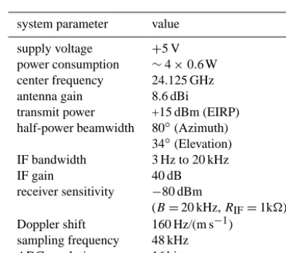
Table 1. Overview of several system parameters of the prototype.

system parameter value

supply voltage +5V power consumption ∼4×0.6W center frequency 24.125GHz antenna gain 8.6dBi transmit power +15dBm (EIRP) half-power beamwidth 80° (Azimuth)

34° (Elevation) IF bandwidth 3Hz to20kHz IF gain 40dB receiver sensitivity −80dBm

(B= 20kHz,RIF= 1kΩ)

Doppler shift 160Hz/(m/s) sampling frequency 48kHz ADC resolution 16bit

the single modules of the radar network. Interfering down-conversion is then filtered out. The analog input stage con-sists of an active anti-aliasing low-pass filter (LPF) with a

3dB cutoff frequency of20kHz, based on a low-noise oper-ational amplifier. The input impedance is1kΩ. This config-uration a receiver sensitivity of−80dBm. A standard stereo-audio codec is used for converting the analog quadrature sig-nal to a digital IQ data stream at a sampling frequency of

fs= 48kHz. Some system parameters of the radar module

and the input stage are given in Table 1, compare RFbeam Microwave GmbH (2011).

As the radar system acts in severe environmental condi-tions with fluid, drizzle, heat etc., hermetically sealed mod-ules are necessary. The enclosures of the radar front-end in Fig. 2 are made from polyethylene and are closed and sealed for the final application. Additionally, they increase the flex-ibility for positioning and tilting of the modules. Coverage

simulations based on deterministic ray-tracing showed that

15° tilting of the modules gives best coverage of the sur-rounding space around the tool (Azodi et al., 2013).

The input stage is built into a metal shielding enclosure. It is supposed to protect the circuit not only against electromag-netic interference but also against the harsh environmental conditions in machine tools. Experiments showed that inter-ference from power supplies and switching electrical actua-tors as well as mechanical vibrations are there to effectively increase the noise level. The high-frequency interference can be suppressed after data acquisition by digital filtering as de-scribed in the next section. The low frequency components in the sub-kilohertz range remains as superimposed interfering signals.

3 Implemented Digital Signal Processing Stage

As the radar modules are based upon a homodyne archi-tecture, the IQ mixer output appears in baseband centered around DC. The analog bandwidth of the active LPF is from

3Hz to20kHz. This covers the needed range of relative ve-locities especially for slowly moving targets.

After digital conversion the signal is buffered and the DC bias is removed. Next a decimation stage follows. It consists of a digital LPF and subsequent downsampling by factor of

M. Figure 4 illustrates the preprocessing steps between ADC and spectral frequency estimation. The digital LPF is a 4th order Chebyshev type I filter with0.25dB ripple andfc= 160Hz cutoff frequency. This cutoff equates to the Doppler shift due to the highest expected relative velocity of1m/s. The filter process reduces the noise contribution, hence the sensitivity level is decreased down to −101dBm.

Each observation window has lengthN Tseconds and is weighted with a window function after decimation.T= 1/fs

is the sampling period andN is the number of sampling points. The decimation process does not change the

observa-Figure 3. Block diagram of the radar system and signal processing components of a single module.

Table 1. Overview of several system parameters of the prototype.

system parameter value

supply voltage +5 V

power consumption ∼4×0.6 W

center frequency 24.125 GHz

antenna gain 8.6 dBi

transmit power +15 dBm (EIRP)

half-power beamwidth 80◦(Azimuth) 34◦(Elevation)

IF bandwidth 3 Hz to 20 kHz

IF gain 40 dB

receiver sensitivity −80 dBm

(B=20 kHz,RIF=1k)

Doppler shift 160 Hz/(m s−1)

sampling frequency 48 kHz

ADC resolution 16 bit

output of the module is the downconverted complex Doppler signal. A frequency gap of 30 MHz between the carrier fre-quencies is introduced by tuning the VCOs to avoid crosstalk between the single modules of the radar network. Interfering down-conversion is then filtered out. The analog input stage consists of an active anti-aliasing low-pass filter (LPF) with a 3 dB cutoff frequency of 20 kHz, based on a low-noise oper-ational amplifier. The input impedance is 1 k. This config-uration allows a receiver sensitivity of−80 dBm. A standard stereo-audio codec is used for converting the analog quadra-ture signal to a digital IQ data stream at a sampling frequency of fs=48 kHz. Some system parameters of the radar mod-ule and the input stage are given in Table 1, compare RFbeam Microwave GmbH (2011).

As the radar system acts in severe environmental condi-tions with fluid, drizzle, heat etc., hermetically sealed mod-ules are necessary. The enclosures of the radar front-end in Fig. 2 are made from polyethylene and are closed and sealed for the final application. Additionally, they increase the flex-ibility for positioning and tilting of the modules. Coverage simulations based on deterministic ray-tracing showed that

15◦ tilting of the modules gives best coverage of the sur-rounding space around the tool (Azodi et al., 2013).

The input stage is built into a metal shielding enclosure. It is supposed to protect the circuit not only against electromag-netic interference but also against the harsh environmental conditions in machine tools. Experiments showed that inter-ference from power supplies, switching electrical actuators and mechanical vibrations are there to effectively increase the noise level. The high-frequency interference can be sup-pressed after data acquisition by digital filtering as described in the next section. Low frequency components in the sub-kilohertz range remains as superimposed interfering signals.

3 Implemented digital signal processing stage

As the radar modules are based upon a homodyne archi-tecture, the IQ mixer output appears in baseband centered around DC. The analog bandwidth of the active LPF is from 3 Hz to 20 kHz. This covers the needed range of relative ve-locities especially for slowly moving targets.

After digital conversion the signal is buffered and the DC bias is removed. Next a decimation stage follows. It con-sists of a digital LPF and subsequent downsampling by fac-tor of M. Figure 4 illustrates the preprocessing steps be-tween ADC and spectral frequency estimation. The digital LPF is a 4th order Chebyshev type I filter with 0.25 dB rip-ple andfc=160 Hz cutoff frequency. This cutoff equates to the Doppler shift due to the highest expected relative velocity of 1 m s−1. The filter process reduces the noise contribution, hence the sensitivity level is decreased down to−101 dBm.

Each observation window has lengthN T seconds and is weighted with a window function after decimation.T =1/fs is the sampling period and N is the number of sampling points. The decimation process does not change the observa-tion period. The new sampling period isTM=MT =M/fs and the number of sampling points isN/M. A Kaiser win-dow with 80 dB sidelobe suppression has proven sufficient selectivity and low spectral leakage. The Kaiser window shape parameter value was chosen asα=3.422.

38 4 T. J. W¨achter, U. Siart, T. F. Eibert and S. Bonerz: Multi-Sensor Doppler Radar for Machine ToolsT. J. Wächter et al.: Multi-sensor Doppler radar for machine tools

ui(k)

uq(k) ·j

from ADC

fs= 48kHz

+ buffer

N T k= 0,1,2, ..

.., N-1

T= 1/fs

LPF

Chebyshev

n= 4 fc= 160Hz

M↓

k′_{= 0,1,2, ..}

.., N/M-1

sample rate

reduction windowKaiser

ˆ S(ν) ν=−L/2, ..

.., L/2-1

short time Fourier transform νctr band-limited spectral centroid

u(k) fs u

′_(k′_),fs

M u′w(k′)

Fig. 4. Preprocessing of complex signal from one single path.

tion period. The new sampling period isTM=M T=M/fs

and the number of sampling points isN/M. A Kaiser win-dow with80dB sidelobe suppression has proven sufficient selectivity and low spectral leakage. The Kaiser window shape parameter value was chosen asα= 3.422.

Frequency resolution is determined by the duration of ob-servation. The number of sampling points for each segment are kept toN∼2n_{for utilization of the efficient}

Radix-2-FFT algorithm. To extract Doppler shift and relative veloc-ity, the short time Fourier spectrum is derived from each data segment by the estimator

ˆ

S(ν) = L−1 X

k′=0

u′

w(k′) exp (−j2πνk′/L), (2)

wherek′_{is an integer andu}′

w(k′)is the preprocessed signal.

The Fourier spectrum is calculated at discrete pointsν, where

ν=−L/2, . . ., L/2−1andL=N/M.

Frequency estimation is based on computation of the band-width limited spectral centroid. The bandband-width for calcula-tion is limited to a window which is identical to the LPF passband, excluding a small guard interval around DC. Ex-ploiting the sign of the received Doppler shift provided by the IQ mixer architecture the integration limits can be set to the frequency indicesνmin< ν < νmaxwhere all indices are

positive for positive Doppler shifts and negative for negative Doppler shifts. The spectral centroid is then calculated only in the frequency interval of interest by

νctr= νmax

P

ν=νmin

ν

Sˆ(ν)

2 νmax P

ν=νmin

Sˆ(ν)

2 . (3)

Limiting the summation in Eq. (3) reduces noise to a min-imum and prevents erroneous biased estimation. In case of multi-target scenarios different methods must be utilized re-garding more than one spectral maximum. But this case is not discussed in this paper since first investigations and per-formance tests assume that there is a single dominant target. Fromνctr the value offˆd=νctrfs/(LM)is calculated.

An estimate for the relative velocity can be obtained with the well-known equationvˆrel= ˆfdλ/2, whereλ=c0/fcis the

wavelength of the corresponding carrier frequencyfc.

Timetin s

F re q u en cy f in H z P o w er S p ec tr al D en si ty S in d B m /H z −150 −100 −50 0 50 100 150 −110 −100 −90 −80 −70 −60 −50 −40

0.5 1 1.5 2 2.5

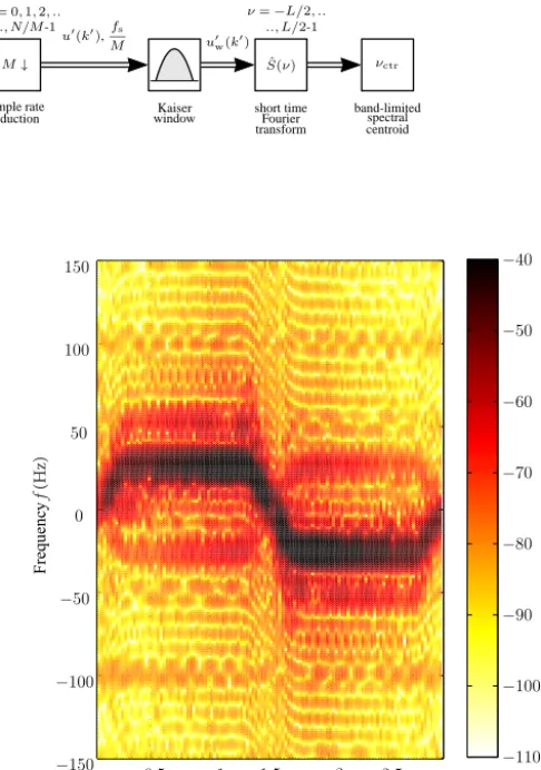
Fig. 5. Doppler spectrogram for a closing and receding movement

of the sensor platform. A metallic sphere serves as reflecting object.

Figure 5 shows a typical spectrogram acquired from the observation of the space in front of a sensor with one single dominant target. This example is based on real measurements performed with the prototype and equipment shown in Fig. 2. In this case the sensor platform is centrally arranged to the sphere and first approaches to it and afterwards departs from it. The spectrogram in Fig. 5 shows a distinct main frequency component. Short phases of acceleration and deceleration at the beginning and the end and a turning point in the middle can be identified.

A critical point for unambiguous detection and tracking of objects are spurious frequency components that are observ-able in Fig. 5. These artifacts arise from IQ imbalance. The origins of this analog signal distortion are fabrication toler-ances of the Schottky diodes and the transmission lines in the

Figure 4. Preprocessing of complex signal from one single path.

Frequency resolution is determined by the duration of ob-servation. The number of sampling points for each segment are kept to N∼2n for utilization of the efficient Radix-2-FFT algorithm. To extract Doppler shift and relative veloc-ity, the short time Fourier spectrum is derived from each data segment by the estimator

ˆ S(ν)=

L−1

X

k0₌₀

u0_w(k0)exp −j2π νk0/L, (2)

wherek0is an integer andu0_w(k0)is the preprocessed signal. The Fourier spectrum is calculated at discrete pointsν, where ν= −L/2, . . . , L/2−1 andL=N/M.

Frequency estimation is based on computation of the band-width limited spectral centroid. The bandband-width for calcula-tion is limited to a window which is identical to the LPF passband, excluding a small guard interval around DC. Ex-ploiting the sign of the received Doppler shift provided by the IQ mixer architecture the integration limits can be set to the frequency indicesνmin< ν < νmaxwhere all indices are positive for positive Doppler shifts and negative for negative Doppler shifts. The spectral centroid is then calculated only in the frequency interval of interest by

νctr=

νmax P ν=νmin ν ˆ S(ν) 2 νmax P ν=νmin ˆ S(ν)

2 . (3)

Limiting the summation in Eq. (3) reduces noise to a min-imum and prevents erroneous biased estimation. In case of multi-target scenarios different methods must be utilized re-garding more than one spectral maximum. But this case is not discussed in this paper since first investigations and per-formance tests assume that there is a single dominant target. Fromνctrthe value offdˆ =νctrfs/(LM)is calculated. An estimate for the relative velocity can be obtained with the well-known equation vrelˆ = ˆfdλ/2, where λ=c0/fc is the wavelength of the corresponding carrier frequencyfc.

Figure 5 shows a typical spectrogram acquired from the observation of the space in front of a sensor with one single dominant target. This example is based on real measurements performed with the prototype shown in Fig. 2. In this case the sensor platform is centrally arranged to the sphere and first approaches to it and afterwards departs from it. The spectro-gram in Fig. 5 shows a distinct main frequency component.

ui(k)

uq(k)

·j from ADC

fs= 48kHz

+ buffer

N T k= 0,1,2, ..

.., N-1

T= 1/fs

LPF

Chebyshev

n= 4

fc= 160Hz

M↓

k′_{= 0,1,2, ..} .., N/M-1

sample rate

reduction windowKaiser

ˆ

S(ν)

ν=−L/2, .. .., L/2-1

short time Fourier transform νctr band-limited_spectral centroid

u(k) fs u

′_(k′_),fs

M u′w(k′)

Fig. 4.Preprocessing of complex signal from one single path.

tion period. The new sampling period isTM=M T=M/fs

and the number of sampling points isN/M. AKaiser

win-dow with 80dB sidelobe suppression has proven sufficient

selectivity and low spectral leakage. The Kaiser window shape parameter value was chosen asα= 3.422.

Frequency resolution is determined by the duration of ob-servation. The number of sampling points for each segment are kept to N∼2n _{for utilization of the efficient}

Radix-2-FFT algorithm. To extract Doppler shift and relative veloc-ity, theshort time Fourier spectrumis derived from each data segment by the estimator

ˆ

S(ν) =

L−1

k′=0

u′

w(k′) exp (−j2πνk′/L), (2)

wherek′is an integer and_u′

w(k′)is the preprocessed signal.

The Fourier spectrum is calculated at discrete pointsν, where

ν=−L/2, . . ., L/2−1andL=N/M.

Frequency estimation is based on computation of the band-width limited spectral centroid. The bandband-width for calcula-tion is limited to a window which is identical to the LPF passband, excluding a small guard interval around DC. Ex-ploiting the sign of the received Doppler shift provided by the IQ mixer architecture the integration limits can be set to the frequency indicesνmin< ν < νmaxwhere all indices are

positive for positive Doppler shifts and negative for negative Doppler shifts. The spectral centroid is then calculated only in the frequency interval of interest by

νctr=

νmax

ν=νmin

ν

Sˆ(ν) 2 νmax

ν=νmin Sˆ(ν)

2 . (3)

Limiting the summation in Eq. (3) reduces noise to a

min-imum and prevents erroneous biased estimation. In case of multi-target scenarios different methods must be utilized re-garding more than one spectral maximum. But this case is

not discussed in this paper since first investigations and pe r-formance tests assume that there is a single dominant target. Fromνctr the value of fˆd=νctrfs/(LM) is calculated.

An estimate for the relative velocity can be obtained with the well-known equationvˆrel= ˆfdλ/2, whereλ=c0/fc is the

wavelength of the corresponding carrier frequencyfc.

Timetin (s)

Freq uen cy f in (H z) Po w er Sp ect ral D en si ty S in dB m /H z −150 −100 −50 0 50 100 150 −110 −100 −90 −80 −70 −60 −50 −40

0.5 1 1.5 2 2.5

Fig. 5.Doppler spectrogram for a closing and receding movement of the sensor platform. A metallic sphere serves as reflecting object.

Figure 5 shows a typical spectrogram acquired from the observation of the space in front of a sensor with one single dominant target. This example is based on real measurements

performed with the prototype and equipment shown in Fig. 2.

In this case the sensor platform is centrally arranged to the

sphere and first approaches to it and afterwards departs from

it. The spectrogram in Fig. 5 shows a distinct main frequency component. Short phases of acceleration and deceleration at the beginning and the end and a turning point in the middle

can be identified.

A critical point for unambiguous detection and tracking of objects are spurious frequency components that are observ-able in Fig. 5. These artifacts arise from IQ imbalance. The origins of this analog signal distortion are fabrication toler-ances of the Schottky diodes and the transmission lines in the

(s) (H z) (dB m/H z) f (H z)

Figure 5. Doppler spectrogram for a closing and receding move-ment of the sensor platform. A metallic sphere serves as reflecting object.

Short phases of acceleration and deceleration at the begin-ning and the end and a turbegin-ning point can be identified.

T. J. Wächter et al.: Multi-sensor Doppler radar for machine toolsT. J. W¨achter, U. Siart, T. F. Eibert and S. Bonerz: Multi-Sensor Doppler Radar for Machine Tools 395

SNR (dB)

v

ar

{

ˆ_f}d

(H

z

2)

N= 1024

N= 2048

N= 4096

0 5 10 15 20 25 30

10-5 10-4 10-3 10-2 10-1 100

Fig. 6. Frequency estimation simulation results for a single com-plex sinusoid with unknown amplitude and phase and the theoreti-cal bounds for estimation variances.fs= 48kHz,fd= 25.6Hz.

mixer stage. Shifts or distortions of the diode characteristic on the one hand and slightly unequal power division or phase deviation from ideal dividers on the other hand are the conse-quences. This causes variations between the output signals of the two mixing units which results in degraded signal qual-ity. Like clutter, spurious peaks potentially increase the false alarm rate considerably. Especially, if solids with fluctuating radar cross section (RCS) have to be detected, e.g. cuboids or cylinders, image components will influence the algorithm performance of the decision unit when this special problem remains unconsidered. This issue is investigated in detail in future work.

4 Single Target Scenario

In a single target scenario with one dominant scatterer at positionr0= (x0, y0)Tthe observed discrete-time Doppler shift signal detected by theith sensor is modeled by

ui_{(k) =A}i_{exp j(Ω}i

dk+ϕi)

+wi_{(k), (4)}

whereΩd=ωdTis the normalized Doppler frequency andw is band-limited measurement and processing noise. Measure-ments reveal thatwis Gaussian white noise with the normal distribution

p(w)_{∼ N}(0,C), (5)

whereCis the noise covariance matrix.

In this application the parametersA,ωdandϕare all un-known. In the following the indexiis omitted. The

Cramer-Rao-Bound (CRB) is a lower bound on the minimum

achiev-able variances depending on the signal properties. In (Rife and Boorstyn, 1974) results for a discrete-time single com-plex sinusoid can be found. The CRB on the variance of the Doppler frequency estimatefdˆ = ˆωd/(2π)is given by

varnfdˆo= 12σ

2

N

(2π)2_A2_T2_N(N2₋₁₎, (6)

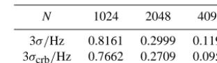
Table 2. Simulation results for the standard deviation:fs= 48kHz,

fd= 25.6Hz,SNR = 10dB.

N 1024 2048 4096

3σ/Hz 0.8161 0.2999 0.1190

3σcrb/Hz 0.7662 0.2709 0.0958

whereσ2

Nis the variance of the noise. The variance offˆd de-pends on theSNR =A2_/σ2

N and the observation timeN T

which is determined by a trade-off between accuracy and agility of signal processing algorithm. Simulation results for a noisy complex sinusoid with varying SNR and various numbers of sampling pointsN are illustrated in Fig. 6, to-gether with the theoretical lower bounds given in Eq. (6).

For low SNR the frequency estimation is distorted and the variance rapidly increases. In Tab. 2 the values for three standard deviations3σof the estimated mean frequency are given. This range includes99.7% of all estimates.

The obtained Doppler frequency shift depends on the sensor-target geometry via the inner product of the distance vector (r0−s) and the velocity vector v= (vx, vy, vz)T.

The equation for the general three-dimensional case with sensor at position(sx, sy, sz)Tis

fd=2

λ

(r0−s)Tv

kr0−sk

, (7)

where_k·krepresents the standard Euclidean vector norm.

4.1 Data Model

In this application a special kind of observation scenario arises. Several sensors are closely spaced on a maneuverable platform and monitor the space in front with one dominant scatterer. This scenario is illustrated in Fig. 7 with the sensor platform and an object inside the closed machine. The plat-form typically moves with constant velocity on straight-lined trajectories.

Compilation of Eq. (7) for a radar network with several distributed sensors results in a system of nonlinear equations of the form

fd=A(ξ) +w. (8)

with the observation matrix A(ξ) which contains the the model of Eq. (7) and the parameter vector ξ= (x, y, z, vx, vy, vz)Tfor the general three-dimensional case.

The number of unknowns is reduced to four as the two-dimensional case is considered. To find the optimalξ∗ _the

constrained minimization problem (e.g., Bjoerk, 1996),

minimize ξ F(ξ)

such thatg(ξ)≤bℓ, ℓ= 1, . . . , p (9) Figure 6. Frequency estimation simulation results for a single

com-plex sinusoid with unknown amplitude and phase and the theoretical bounds for estimation variances.fs=48 kHz,fd=25.6 Hz.

4 Single target scenario

In a single target scenario with one dominant scatterer at positionr0=(x0, y0, )Tthe observed discrete-time Doppler shift signal detected by theith sensor is modeled by

ui(k)=Aiexpj(_dik+ϕi)+wi(k), (4) whered=ωdT is the normalized Doppler frequency andw is band-limited measurement and processing noise. Measure-ments reveal thatwis Gaussian white noise with the normal distribution

p(w)∼N(0,C), (5)

where C is the noise covariance matrix.

In this application the parametersA,ωdandϕare all un-known. In the following the indexiis omitted. The Cramer-Rao-Bound (CRB) is a lower bound on the minimum achiev-able variances depending on the signal properties. In (Rife and Boorstyn, 1974) results for a discrete-time single com-plex sinusoid can be found. The CRB on the variance of the Doppler frequency estimatefdˆ = ˆωd/(2π )is given by

varnfdˆo= 12σ 2 N

(2π )2_A2_T2_{N (N}2₋₁₎, (6) whereσ_N2 is the variance of the noise. The variance offˆd de-pends on the SNR=A2/σ_N2 and the observation timeN T which is determined by a trade-off between accuracy and agility of signal processing algorithm. Simulation results for a noisy complex sinusoid with varying SNR and various numbers of sampling points N are illustrated in Fig. 6, to-gether with the theoretical lower bounds given by Eq. (6).

For low SNR the frequency estimation is distorted and the variance rapidly increases. In Tab. 2 the values for three standard deviations 3σ of the estimated mean frequency are given. This range includes 99.7 % of all estimates.

The obtained Doppler frequency shift depends on the sensor-target geometry via the inner product of the distance

Table 2. Simulation results for the standard deviation:fs=48 kHz,

fd=25.6 Hz, SNR=10 dB.

N 1024 2048 4096

3σ/Hz 0.8161 0.2999 0.1190

3σcrb/Hz 0.7662 0.2709 0.0958

vector(r0−s)and the velocity vectorv=(vx, vy, vz)T. The

equation for the general three-dimensional case with sensor at position(sx, sy, sz)Tis

fd= 2 λ

(r0−s)Tv kr0−sk

, (7)

wherek·krepresents the standard Euclidean vector norm. 4.1 Data model

In this application a special kind of observation scenario arises. Several sensors are closely spaced on a maneuver-able platform monitoring the space in front with one dom-inant scatterer. Figure 7 illustrates the scenario with sensor platform and object inside the closed machine. The platform typically moves with constant velocity on straight-lined tra-jectories.

Compilation of Eq. (7) for a radar network with several distributed sensors results in a system of nonlinear equations

fd=A(ξ)+w. (8)

with the observation matrix A(ξ) which contains the the model of Eq. (7) and the parameter vector ξ= (x, y, z, vx, vy, vz)Tfor the general three-dimensional case.

The number of unknowns is reduced to four as the two-dimensional case is considered. To find the optimalξ∗ the constrained minimization problem (e.g., Bjoerk, 1996), minimize

ξ F (ξ)

such thatg(ξ)≤b`, `=1, . . . , p (9)

has to be solved, whereF (ξ)is the cost function and g(ξ) contains linear and nonlinear constraints for maximum dis-tances between sensor and object and maximum velocities in all directions. To solve this nonlinear minimization problem and to find a solution for positionr0and velocity of the plat-formv, Newton-type or Gauss-Newton method is applied. A fundamental problem is to find the global minimum. For cost functions and their Jacobian with several minima, the accu-racy of the results strongly depend on the initial guess. More advanced methods are necessary which find the global min-imum, e.g. grid search methods. These account for higher computing capacity at the beginning of a new trajectory. Then, the previously found solutions can be used recursively. The problem is investigated in detail in future works.

40 T. J. Wächter et al.: Multi-sensor Doppler radar for machine tools

machine enclosure

observed space

sensor platform

x

y

object

Fig. 7. Illustration of a typical scenario of the application: One dom-inant scatterer at fixed position and the maneuverable sensor plat-form with radar modules. Arrows point out the typical rectilinear motions during manual operation.

has to be solved, where

F

(

ξ

)

is the cost function and

g

(

ξ

)

contains linear and nonlinear constraints for maximum

dis-tances between sensor and object and maximum velocities in

all directions.

To solve this nonlinear minimization problem and to find

a solution for position

r

and velocity of the platform

v

,

Newton-type or Gauss-Newton method is applied. A

funda-mental problem is to find the global minimum. For cost

func-tions and their Jacobian with several minima, the accuracy

of the results strongly depend on the initial guess. More

ad-vanced methods are necessary which find the global

mini-mum, e.g. grid search methods. These account for higher

computing capacity at the beginning of a new trajectory.

Then, the previously found solutions can be used recursively.

The problem is investigated in detail in future works.

In the next section measurement data of a one-dimensional

linear motion are analyzed to show the accuracy of the

fre-quency estimation. The second example investigates a

two-dimensional scenario. A nonlinear solver is used to obtain

position estimates from synthetic and measurement data.

4.2

Measurement Results for Linear Motion

This section provides the results of the algorithm applied to

a set of measurements. The measurements are done with the

in-house developed prototype depicted in Fig. 2. They

clar-ify quality and accuracy of the algorithm for frequency

esti-mation. The received signal streams are stored and available

for off-line post processing. To obtain sufficient frequency

resolution the processed block size is set to

N

= 4096

data

points. This results in a resolution of

1

/

(

N T

)

≈

11

.

7

Hz

dur-Timet(s)

E

st

im

at

ed

v

el

o

ci

ty

vx

(m

/s

)

estimatedvx(s1)

estimatedvx(s2)

estimatedvx(s3)

estimatedvx(s4)

machine datavx

0 0_.4 0_.8 1_.2 1.6 2 2_.4

−0_.5

−0.4

−0_.3

−0_.2

−0.1

0

0_.1

0_.2

0.3

0_.4

0_.5

Fig. 8. Estimated velocity from Doppler shift measurements for an axial movement of the sensor platform.

by overlapped data segments. Measurement and reference

data for position and speed of the sensor platform with the

same update rate of

4

ms are used for performance tests with

the prototype. Reference data available from the machine

tool control unit provides exact position and velocity data.

Results of the following scenario are presented:

Compara-ble to Figs. 1 and 2, the sensor platform is equipped with four

sensors. The movement of the sensor platform is

bidirection-ally (i.e. back and forth) on an axial path. A metal sphere with

a diameter

d

= 15

cm serves as scattering object. Its position

is fixed and aligned to the center of the platform. As the

cir-cumference of the sphere is much larger than the wavelength,

the RCS of the sphere is in the optical region and equal the

cross-section area

d

_π/

₄

_{of the sphere.}

Referred to the coordinate system in Fig. 1 the

veloci-tiy components

v

and

v

of the platform are both equal to

zero and the

y

- and

z

-coordinates remain constant. Figure 8

shows the obtained velocity from the internal machine’s

con-trol unit (solid graph) and the estimated velocity

v

(dashed

and dotted graphs) from the data of each of the four sensors.

The small time shifts between the various sensor streams

come from the data acquisition procedure. The exact value

is known and can be compensated. At the beginning a

reced-ing movement is identified (negative sign) with continuously

increasing velocity up to a deceleration phase around

0

.

35

s

to

0

.

45

s. Then, the turning point is reached and the

move-ment with positive acceleration and velocity follows (positive

sign). The movement pattern is repeated three times. Against

the background of a dynamic scenario with ever-changing

velocity, the estimates are in very good agreement with the

true velocity in Fig. 8. In this scenario velocities of

0

.

47

m/s

and accelerations up to

6

.

5

m/s

are reached.

Minor discrepancy can be identified at the turning points

dominant scatterer at fixed position and the maneuverable sensor platform with radar modules. Arrows point out the typical rectilin-ear motion during manual operation.

In the next section measurement data of a one-dimensional linear motion are analyzed to show the accuracy of the fre-quency estimation. The second example investigates a two-dimensional scenario. A nonlinear solver is used to obtain position estimates from synthetic and measurement data. 4.2 Measurement results for linear motion

This section provides the results of the algorithm applied to a set of measurements. The measurements are done with the in-house developed prototype depicted in Fig. 2. They clarify quality and accuracy of the algorithm for frequency estima-tion. The received signal streams are stored and available for off-line post processing. To obtain sufficient frequency reso-lution the processed block size is set toN=4096 data points. This results in a resolution of 1/(N T )≈11.7 Hz during the post processing. The decimation process has no influence on the value ofN T. Variable update rates are achieved by over-lapped data segments. Measurement and reference data for position and speed of the sensor platform with the same up-date rate of 4 ms are used for performance tests with the pro-totype. Reference data available from the machine tool con-trol unit provides exact position and velocity data.

Results of the following scenario are presented: Compara-ble to Figs. 1 and 2, the sensor platform is equipped with four sensors. The movement of the sensor platform is bidirection-ally (i.e. back and forth) on an axial path. A metal sphere with a diameterd=15 cm serves as scattering object. Its position is fixed and aligned to the center of the platform. As the cir-cumference of the sphere is much larger than the wavelength, the RCS of the sphere is in the optical region and equal the cross-section aread2π/4 of the sphere.

machine enclosure

observed space

sensor platform

x

y

object

Fig. 7. Illustration of a typical scenario of the application: One dom-inant scatterer at fixed position and the maneuverable sensor plat-form with radar modules. Arrows point out the typical rectilinear motions during manual operation.

has to be solved, whereF(ξ)is the cost function andg(ξ)

contains linear and nonlinear constraints for maximum dis-tances between sensor and object and maximum velocities in all directions.

To solve this nonlinear minimization problem and to find a solution for position r0 and velocity of the platform v,

Newton-type or Gauss-Newton method is applied. A

funda-mental problem is to find the global minimum. For cost func-tions and their Jacobian with several minima, the accuracy of the results strongly depend on the initial guess. More ad-vanced methods are necessary which find the global mini-mum, e.g. grid search methods. These account for higher computing capacity at the beginning of a new trajectory. Then, the previously found solutions can be used recursively. The problem is investigated in detail in future works.

In the next section measurement data of a one-dimensional linear motion are analyzed to show the accuracy of the fre-quency estimation. The second example investigates a two-dimensional scenario. A nonlinear solver is used to obtain position estimates from synthetic and measurement data.

4.2 Measurement Results for Linear Motion

This section provides the results of the algorithm applied to a set of measurements. The measurements are done with the in-house developed prototype depicted in Fig. 2. They clar-ify quality and accuracy of the algorithm for frequency esti-mation. The received signal streams are stored and available for off-line post processing. To obtain sufficient frequency resolution the processed block size is set toN = 4096data points. This results in a resolution of1/(N T)_≈11.7Hz dur-ing the post processdur-ing. The decimation process has no influ-ence on the value ofN T. Variable update rates are achieved

Timet(s)

E

st

im

at

ed

v

el

o

ci

ty

vx

(m

/s

)

estimatedvx(s1)

estimatedvx(s2)

estimatedvx(s3)

estimatedvx(s4)

machine datavx

0 0.4 0.8 1.2 1.6 2 2.4 −0.5

−0.4 −0.3 −0.2 −0.1 0 0.1 0.2 0.3 0.4 0.5

Fig. 8. Estimated velocity from Doppler shift measurements for an axial movement of the sensor platform.

by overlapped data segments. Measurement and reference data for position and speed of the sensor platform with the same update rate of4ms are used for performance tests with the prototype. Reference data available from the machine tool control unit provides exact position and velocity data.

Results of the following scenario are presented: Compara-ble to Figs. 1 and 2, the sensor platform is equipped with four sensors. The movement of the sensor platform is bidirection-ally (i.e. back and forth) on an axial path. A metal sphere with a diameterd= 15cm serves as scattering object. Its position is fixed and aligned to the center of the platform. As the cir-cumference of the sphere is much larger than the wavelength, the RCS of the sphere is in the optical region and equal the cross-section aread2_{π/4of the sphere.}

Referred to the coordinate system in Fig. 1 the veloci-tiy componentsvy andvz of the platform are both equal to

zero and they- andz-coordinates remain constant. Figure 8 shows the obtained velocity from the internal machine’s con-trol unit (solid graph) and the estimated velocityvx(dashed

and dotted graphs) from the data of each of the four sensors. The small time shifts between the various sensor streams come from the data acquisition procedure. The exact value is known and can be compensated. At the beginning a reced-ing movement is identified (negative sign) with continuously increasing velocity up to a deceleration phase around0.35s to0.45s. Then, the turning point is reached and the move-ment with positive acceleration and velocity follows (positive sign). The movement pattern is repeated three times. Against the background of a dynamic scenario with ever-changing velocity, the estimates are in very good agreement with the true velocity in Fig. 8. In this scenario velocities of0.47m/s and accelerations up to6.5m/s2are reached.

Minor discrepancy can be identified at the turning points where the velocities and change in position becomes small. This is due to the limited frequency resolution. Frequencies

Figure 8. Estimated velocity from Doppler shift measurements for an axial movement of the sensor platform.

Referred to the coordinate system in Fig. 1 the veloci-tiy componentsvy andvz of the platform are both equal to

zero and they andzcoordinates remain constant. Figure 8 shows the obtained velocity from the internal machine’s con-trol unit (solid graph) and the estimated velocityvx (dashed

and dotted graphs) from the data of each of the four sensors. The small time shifts between the various sensor streams come from the data acquisition procedure. The exact value is known and can be compensated. At the beginning a reced-ing movement is identified (negative sign) with continuously increasing velocity up to a deceleration phase around 0.35 to 0.45 s. Then, the turning point is reached and the move-ment with positive acceleration and velocity follows (pos-itive sign). The movement pattern is repeated three times. Against the background of a dynamic scenario with ever-changing velocity, the estimates are in very good agreement with the true velocity in Fig. 8. In this scenario velocities of 0.47 m s−1and accelerations up to 6.5 m s−2are reached.

Minor discrepancy can be identified at the turning points where the velocities and change in position becomes small. This is due to the limited frequency resolution. Frequencies lower than 11.7 Hz (corresponding to∼73.1 mm s−1in this system) are actually mapped to zero due to lack of accuracy of the estimate. Improvements are achieved by using adap-tive parallel analyzing of longer sequences and subsequent adjustment of the position.

4.3 Results for diagonal motion

As a further scenario a two-dimensional motion is investi-gated. Figure 9 shows the results for a diagonal approaching motion wherevx andvy are nonzero. Using the coordinate

system of Fig. 1, the starting position of the object (sphere, d=15 cm) is at (0.5 m, 0.5 m, 0)Tand the constant velocity of the sensor platform is (−0.707 m s−1,−0.707 m s−1, 0)T. The position of the object is represented by circles. The results for synthetic data (+) and for real measurement data

T. J. Wächter et al.: Multi-sensor Doppler radar for machine tools 41 T. J. W¨achter, U. Siart, T. F. Eibert and S. Bonerz: Multi-Sensor Doppler Radar for Machine Tools 7

y(m)

x

(m

)

true position synthetic data measurement data sensor position

0.5 0.25 0 ₋0.25 ₋0.5 0.6

0 0.1 0.2 0.3 0.4 0.5

Fig. 9. Target localization close to the sensor platform. The initial guess of the parameter vector for the iterative nonlinear solver is (0.91m,0.53m,0,−0.66m/s,−0.33m/s,0)T.

lower than 11.7Hz (corresponding to _∼73.1mm/s in this system) are actually mapped to zero due to lack of accuracy of the estimate. Improvements are achieved by using adap-tive parallel analyzing of longer sequences and subsequent adjustment of the position.

4.3 Results for Diagonal Motion

As a further scenario a two-dimensional motion is investi-gated. Figure 9 shows the results for a diagonal approaching motion wherevxandvy are nonzero. Using the coordinate

system of Fig. 1, the starting position of the object (sphere, d= 15cm) is at(0.5m,0.5m,0)T_{and the constant velocity} of the sensor platform is(−0.707m/s,−0.707m/s,0)T_{. The} position of the object is represented by circles. The results for synthetic data (+) and for real measurement data (⋄_{) are}

very similar and close to the real position of the object. The algorithm is based on the approach of Chan and Jar-dine (1990) which uses a special cost function involving the time derivative of the Doppler shiftf˙d(rate of change). For further details the reader is referred to the original paper.

In this example the absolute errors between real and esti-mated position are lower than4cm, what is already sufficient for collision warning in machine tools. Further investigations are in progress to improve reliability and flexibility of the al-gorithm to make it applicable for arbitrary linear motions.

5 Conclusions

This paper presented an implementation of a prototype sys-tem that aims at a new application of24GHz CW radar tech-nology in machine tools of collision detection and avoid-ance. Important aspects for the mechanical design, the RF hardware, the components for the baseband processing and the elements of the developed algorithm for velocity estima-tion have been described.This first approach treats single-target scenarios in a two-dimensional space.For validation

the case of linear motion has been investigated. Results from conducted measurements reveal very good agreement of ve-locity estimates with the reference data provided by the ma-chine’s control unit. The application of a nonlinear solver for position estimation in a two-dimensional motion scenario showed acceptably low position estimation errors. This pro-totype system serves as the basis for further investigations and developments towards a multi-sensor radar system for fast collision detection in machine tools.Due to the rather weak sensitivity of the used modules and the coarse Doppler resolution due to short observation windows the effect of multiple targets and multiple reflections has not been con-sidered. It is expected that this simple approach is suitable for the majority of collision scenarios. However, specifica-tion of the actual false alarm and missed detecspecifica-tion rates re-quires further studies. Further topics for future work are ex-tension to three dimensions, the question of the minimum necessary number of sensors for uniqueness of the solution, and their optimum positioning around the tool. Although the observation time is very short in this application the effect of cross section fluctuations also needs further investigations.

Acknowledgements. The authors would like to thank Dipl.-Ing.

Matthias Berger and Dipl.-Ing. Dennis Korff from the Institute of Production Management, Technology and Machine Tools (PTW) of the Technische Universit¨at Darmstadt for their help and support during the execution of the measurements.

This work is funded by the Bavarian Ministry of Economic Af-fairs and Media, Energy and Technology within the economic development scheme ”Mikrosystemtechnik Bayern” under grant BAY158/002.

References

Abele, E., Brecher, C., Gsell, S.C., Hassis, A. and Korff, D.: Steps towards a protection system for machine tool main spindles against crash-caused damages, Springer J. Prod. Eng., 6.6, 631-642, doi:10.1007/s11740-012-0422-6, 2012.

Azodi, H., Siart, U. and Eibert, T.F.: A fast three-dimensional de-terministic ray tracing coverage simulator for a 24 GHz anti-collision radar, Adv. Radio Sci., 11(4), 55-60, doi:10.5194/ars-11-55-2013, 2013.

Barton, D. K.: Radar System Analysis, 1. Ed., Prentice Hall, 1964. Bj¨orck, ˚A.: Numerical Methods for Least Squares Problems, 1.

Ed., Society for Industrial and Applied Mathematics (SIAM), doi:10.1137/1.9781611971484, 1996.

Chan, Y.-T. and Jardine, F.L.:, Target localization and tracking from Doppler-shift measurements, IEEE J. Oceanic Eng., 15(3), 251-257, doi:10.1109/48.107154, 1990.

RFbeam Microwave GmbH: K-LC2 Radar Transceiver - Datasheet, Revision: May-2011. available at: www.rfbeam.ch.

Rife, D. and Boorstyn, R.R.: Single tone parameter estimation from discrete-time observations, IEEE Trans. Inf. Theory, 20(5), 591-598, doi:10.1109/TIT.1974.1055282, 1974.

Figure 9. Target localization close to the sensor platform. The initial guess of the parameter vector for the iterative nonlinear solver is (0.91 m, 0.53 m, 0,−0.66 m s−1,−0.33 m s−1, 0)T.

() are very similar and close to the real position of the ob-ject.

The algorithm is based on the approach of Chan and Jar-dine (1990) which uses a special cost function involving the time derivative of the Doppler shiftfd˙ (rate of change). For further details the reader is referred to the original paper.

In this example the absolute errors between real and esti-mated position are lower than 4 cm, what is already sufficient for collision warning in machine tools. Further investigations are in progress to improve reliability and flexibility of the al-gorithm to make it applicable for arbitrary linear motions.

5 Conclusions

This paper presented an implementation of a prototype sys-tem that aims at a new application of 24 GHz CW radar tech-nology in machine tools of collision detection and avoid-ance. Important aspects for the mechanical design, the RF hardware, the components for the baseband processing and the elements of the developed algorithm for velocity estima-tion have been described. This first approach treats single-target scenarios in a two-dimensional space. For validation the case of linear motion has been investigated. Results from conducted measurements reveal very good agreement of ve-locity estimates with the reference data provided by the ma-chine’s control unit. The application of a nonlinear solver for position estimation in a two-dimensional motion scenario showed acceptably low position estimation errors. This pro-totype system serves as the basis for further investigations and developments towards a multi-sensor radar system for fast collision detection in machine tools. Due to the rather weak sensitivity of the used modules and the coarse Doppler resolution due to short observation windows the effect of multiple targets and multiple reflections has not been con-sidered. It is expected that this simple approach is suitable for the majority of collision scenarios. However, specifica-tion of the actual false alarm and missed detecspecifica-tion rates re-quires further studies. Further topics for future work are

ex-tension to three dimensions, the question of the minimum necessary number of sensors for uniqueness of the solution, and their optimum positioning around the tool. Although the observation time is very short in this application the effect of cross section fluctuations also needs further investigations.

Acknowledgements. The authors would like to thank M. Berger and

D. Korff from the Institute of Production Management, Technology and Machine Tools (PTW) of the Technische Universität Darmstadt for their help and support during the execution of the measurements. This work is funded by the Bavarian Ministry of Economic Affairs and Media, Energy and Technology within the economic development scheme “Mikrosystemtechnik Bayern” under grant BAY158/002.

Edited by: U. van Rienen

Reviewed by: two anonymous referees

References

Abele, E., Brecher, C., Gsell, S. C., Hassis, A., and Korff, D.: Steps towards a protection system for machine tool main spin-dles against crash-caused damages, Springer J. Prod. Eng., 6.6, 631–642, doi:10.1007/s11740-012-0422-6, 2012.

Azodi, H., Siart, U., and Eibert, T. F.: A fast three-dimensional deterministic ray tracing coverage simulator for a 24 GHz anti-collision radar, Adv. Radio Sci., 11, 55–60, doi:10.5194/ars-11-55-2013, 2013.

Barton, D. K.: Radar System Analysis, 1. Ed., Prentice Hall, 1964. Björck, Å.: Numerical Methods for Least Squares Problems, 1.

Ed., Society for Industrial and Applied Mathematics (SIAM), doi:10.1137/1.9781611971484, 1996.

Chan, Y.-T. and Jardine, F. L.:, Target localization and tracking from Doppler-shift measurements, IEEE J. Oceanic Eng., 15, 251– 257, doi:10.1109/48.107154, 1990.

RFbeam Microwave GmbH: K-LC2 Radar Transceiver – Datasheet, available at: http://www.rfbeam.ch (last access: 12 July 2013), 2011.

Rife, D. and Boorstyn, R. R.: Single tone parameter estimation from discrete-time observations, IEEE Trans. Inf. Theory, 20, 591– 598, doi:10.1109/TIT.1974.1055282, 1974.

Skolnik, M. I.: Theoretical accuracy of radar measurements, IRE Trans. Aeronaut. Navig. Electron., ANE-7.4, 123–129, doi:10.1109/TANE3.1960.4201757, 1960.

Strohm, K. M., Bloecher, H.-L., Schneider, R., and Wenger,

J., Development of future short range radar

tech-nology, European Radar Conference 2005, 165–168,

doi:10.1109/EURAD.2005.1605591, 2005.