R E S E A R C H
Open Access
The relationship between multi-objective
robustness concepts and set-valued
optimization
Jonas Ide
1, Elisabeth Köbis
2, Daishi Kuroiwa
3, Anita Schöbel
1and Christiane Tammer
4*Dedicated to Prof. W. Takahashi on the occasion of his 70th birthday
*Correspondence:
christiane.tammer@mathematik. uni-halle.de
4Martin-Luther-University
Halle-Wittenberg, Halle, Germany Full list of author information is available at the end of the article
Abstract
In this paper, we discuss the connection between concepts of robustness for multi-objective optimization problems and set order relations. We extend some of the existing concepts to general spaces and cones using set relations. Furthermore, we derive new concepts of robustness for multi-objective optimization problems. We point out that robust multi-objective optimization can be interpreted as an
application of set-valued optimization. Furthermore, we develop new algorithms for solving uncertain multi-objective optimization problems. These algorithms can be used in order to solve a special class of set-valued optimization problems.
Keywords: robust optimization; multi-objective optimization; scalarization; vectorization; set-valued optimization
1 Introduction
Dealing with uncertainty in multi-objective optimization problems is very important in many applications. On the one hand, most real world optimization problems are contam-inated with uncertain data, especially traffic optimization problems, scheduling problems, portfolio optimization, network flow and network design problems. On the other hand, many real world optimization problems require the minimization of multiple conflicting objectives (see []),e.g.the maximization of the expected return versus the minimization of risk in portfolio optimization, the minimization of production time versus the mini-mization of the cost of manufacturing equipment, or the maximini-mization of tumor control versus the minimization of normal tissue complication in radiotherapy treatment design. For an optimization problem contaminated with uncertain data it is typical that at the time it is solved these data are not completely known. It is very important to estimate the effects of this uncertainty and so it is necessary to evaluate how sensitive an optimal solu-tion is to perturbasolu-tions of the input data. One way to deal with this quessolu-tion issensitivity analysis(for an overview see []). Sensitivity analysis is an a posteriori approach and pro-vides ranges for input data within which a solution remains feasible or optimal. It does not, however, provide a course of action for changing a solution should the perturbation be outside this range. In contrast,stochastic programming (seee.g.Birge and Louveaux [] for an introduction) androbust optimization(seee.g.[, ] for an overview) take the uncertainty into account during the optimization process. While stochastic programming
assumes some knowledge about the probability distribution of the uncertain data and the objective usually is to find a solution that is feasible with a certain probability and that op-timizes the expected value of some objective function, robust optimization hedges against the worst case. Hence robust optimization does not require any probabilistic information. Depending on the concrete application one can decide whether robust or stochastic opti-mization is the more appropriate way of dealing with uncertainty.
Robust optimization is usually applied to problems where a solution is required which hedges against all possible scenarios. For example, the emergency department with land-ing place for rescue helicopters in a ski resort should be chosen in such a way that the flight time to all ski slopes in the resort that are to be protected is minimized in the worst case, even though flight times are uncertain due to unknown weather conditions. Similarly, if an aircraft schedule of an airline is to be determined, one would want to be able to provide service to as many passengers as possible in a cost-effective manner, even though the exact number of passengers is not known at the time the schedule is fixed.
Generally, in the concept of robustness it is not assumed that all data are known, but one allows different scenarios for the input parameters and looks for a solution that works well in every uncertain scenario.
Unfortunately, at the time the uncertain optimization problem has to be solved, it is not known which scenario is going to be realized. Therefore, a definition of a ‘good’ (or robust against the perturbations in the uncertain parameter) solution is necessary.
Robust optimization is a growing field of research, we refer to Ben-Tal, El Ghaoui, Ne-mirovski [], Kouvelis and Yu [] for an overview of results and applications for the most prominent concepts. Several other concepts of robustness were introduced more recently, e.g.the concept of light robustness by Fischetti and Monaci [] or the concept of recovery-robustness in Liebchenet al.[], for a unified approach, see []. A scenario-based approach is suggested in Goerigk and Schöbel []. In all these approaches, the uncertain optimiza-tion problem is replaced by a deterministic version, called therobust counterpartof the uncertain problem.
One of the most common approaches is the concept of minmax robustness, introduced by Soyster [] and studiede.g.by Ben-Tal and Nemirovski []. Here, a solution is said to be robust, if it minimizes the worst case of the objective function over all scenarios. We do not go into detail here as for this paper we mostly consider concepts of robustness for multi-objective optimization problems.
Now, if we consider the objective function in the problem definition to be not a single-objective, but a multi-objective function, the concepts of robustness do not apply natu-rally anymore. The problem obviously is that there is no total order onRk and the ro-bustness concepts for uncertain single-objective optimization problems rely on the total order ofR. Therefore, new definitions of what is seen as a robust solution to an uncertain multi-objective optimization problem are necessary.
introduced the degree of robustness as a measure how much a predefined neighborhood of the considered solution can be extended without containing solutions whose function values are too bad. An overview of the existing concepts of robustness for multi-objective optimization problems can be found in [] and [].
A first approach to extending the concept of minmax robustness to multi-objective opti-mization was presented by Kuroiwa and Lee []. Here, the worst case in each component is calculated separately, and an efficient solution to the problem of minimizing the vec-tor of worst cases is then called a robust solution to the original problem. This definition has been extended by Ehrgott,et al.[], where the authors replace the objective function by a set-valued objective function. Furthermore, the authors present solution algorithms for calculating minmax-robust efficient solutions, one of which is closely connected to the concept of robustness presented by Kuroiwa and Lee []. Furthermore, in [] the authors present solution concepts for obtaining robust points of uncertain multi-objective opti-mization problems and study optimality conditions for the special case of convex objective functions in [].
Set-valued optimization deals on the other hand with the problem of minimizing a func-tion where the image of a point is in fact a set. Minimizing a set is not totally intuitive since on a power set there is no total order as well as onRk. Therefore, a definition of what can
be seen as an optimal solution to minimizing a set-valued objective function is neces-sary. In order to compare sets, several preorders have been introduced (seee.g.[–]). With these preorders it is then possible to formulate set-valued optimization problems related to robustness for multi-objective optimization problems, especially, we show that the concept of minmax-robust efficiency (see []) is closely connected to a certain set order relation, introduced by Kuroiwa [, ], namely theupper-type set relation. We derive our results in general spaces using arguments from nonlinear and convex analysis (see Takahashi [, ]), for methods from numerical analysis in general spaces, seee.g. Aoyama, Kohsaka, Takahashi [], Takahashi [].
Replacing the set order relation implicitly used in the definition of minmax-robust ef-ficiency, Ide and Köbis [] presented various other concepts of robustness for multi-objective optimization, derived by replacing the upper-type set relation with another set ordering from the literature.
Now, this paper is structured as follows: After fixing the notation and recalling the def-initions of set order relations in Section , in Section we introduce several concepts of robustness for multi-objective optimization problems based on set order relations. We show some characterizations for robust solutions in the sense of set-valued optimization that are important for deriving solution procedures using the ideas given in []. A lot of the results presented in [] can be extended to our general setting. Using this informa-tion, we extend the algorithms presented in [] to concepts for robustness and then we use these algorithms in order to solve a certain class of set-valued optimization problems. We conclude the paper with some final remarks and an outlook to future research.
2 Preliminaries
C#:={y∗∈C∗| ∀y∈C\ {}:y∗(y) > }. Furthermore, letXbe a linear space,F:X⇒Y (with the ‘⇒’-notation we denote thatFis a set-valued objective function whose function values are sets inY), andXa subset ofX. As usual, we denote the graph of the set-valued mapFbygraphF:={(x,y)∈X×Y|y∈F(x)}. Furthermore, we defineF(X) :=x∈XF(x). In set optimization, the following set relations play an important role; see Young [], Nishnianidze [], Kuroiwa [, , ], Jahn and Ha [] and Eichfelder and Jahn []. We will use these set relations to introduce several concepts of robustness.
Definition (Set less order relation [, , ]) LetC⊂Y be a proper closed convex and pointed cone. Furthermore, letA,B⊂Y be arbitrarily chosen sets. Then the set less order relation is defined by
A sCB:⇐⇒A⊆B–CandA+C⊇B.
Remark Of course, we have
A⊆B–C⇐⇒ ∀a∈A∃b∈B:a≤Cb
and
A+C⊇B⇐⇒ ∀b∈B∃a∈A:a≤Cb.
Definition (Upper-type set relation [, ]) LetA,B⊂Ybe arbitrarily chosen sets and C⊂Ya proper closed convex and pointed cone. Then theu-type set relation u
Cis defined
by
A uCB:⇐⇒A⊆B–C⇐⇒ ∀a∈A∃b∈B:a≤Cb.
Another important set order relation is the lower-type set relation:
Definition (Lower-type set relation [, ]) LetA,B⊂Ybe arbitrarily chosen sets and
C⊂Ya proper closed convex and pointed cone. Then thel-type set relation lCis defined by
A l
CB:⇐⇒A+C⊇B⇐⇒ ∀b∈B∃a∈A:a≤Cb.
Remark Note that the conditions
(i) A⊂B–intC,
(ii) A+N⊂B–Cfor some neighborhoodNof the zero vectorY inY
are not equivalent whenAis not compact. Clearly (ii) implies (i) ifintC=∅. From a theo-retical viewpoint, (ii) may, in some cases, be more appropriate for describing solutions.
Remark There is the following relationship between thel-type set relation lCand the u-type set relation u
–C:
A lCB:⇐⇒A+C⊇B⇐⇒B⊆A– (–C)⇐⇒:B u–CA.
To conclude the notation, we introduce a set-valued optimization problem: Consider F:X⇒Y, andX a subset ofX. Furthermore, let be a preorder on the power set ofY given by Definition , , , respectively. Then a set-valued optimization problem (SP– ) is given by
(SP– ) -minimizeF(x), subject tox∈X,
where minimal solutions of (SP– ) are defined in the following way:
Definition (Minimal solutions of (SP– ) w.r.t. the preorder ) Given a set-valued
optimization problem (SP– ), an elementx∈Xis called a minimal solution to (SP– ) if
F(x) F(x) for somex∈X⇒F(x) F(x).
Remark If we use the set relation lCintroduced in Definition in the formulation of the solution concept,i.e., we study the set-valued optimization problem of (SP– l
C),
we observe that this solution concept is based on comparisons among sets of minimal points of values ofF. Furthermore, considering theu-type set relation uC(Definition ), i.e., considering the problem (SP– u
C) we recognize that this solution concept is based
on comparisons among sets of maximal points of values ofF. Whenx∈X is a minimal solution of problem (SP– lC) there does not existx∈Xsuch thatF(x) is strictly smaller thanF(x) with respect to the set order l
C.
Furthermore, the following definition of a minimizer of a set-valued optimization prob-lem is very often used in the theory of set optimization and given below. However, the solution concept introduced in Definition is more natural and useful as we can see in Example .
In the next definition we use the set of minimal elements of a nonempty subsetAofY with respect toC:
Min(A,C) :=y∈A|A∩(y–C\ {}=∅.
Definition (Minimizer of a set-valued optimization problem) Letx∈X and (x,y)∈
graphF. The pair (x,y)∈graphFis called a minimizer ofF:X⇒YoverXwith respect to Cify∈Min(F(X),C).
For our approach to robustness of uncertain multi-objective optimization problems, minimal solutions in the sense of Definition are useful and therefore, when consider-ing robustness concepts, we will deal with this solution concept in the followconsider-ing.
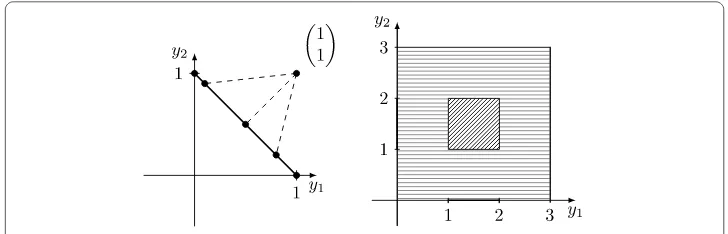
Figure 1 Feasible solution sets ofF1,F2, described in Examples 1 and 2.
Example Consider the set-valued optimization problem
(SP– lC) lC-minimizeF(x), subject tox∈X,
withX=R,Y=R,C=R
+,X= [, ] andF:X⇒Yis given by
F(x) :=
[(, ), (, )] ifx= , [( –x,x), (, )] ifx∈(, ],
where [(a,b), (c,d)] is the line segment between (a,b) and (c,d). Only the elementx= is a minimal solution of (SP– lC). However, all elements (x,y)∈graphFwithx∈[, ],y= ( –x,x) forx∈(, ] andy= (, ) forx= are minimizers of the set-valued optimization problem in the sense of Definition . This example shows that the solution concept with respect to the set relation l
C(see Definitions and ) is more natural and useful than the
concept of minimizers introduced in Definition .
Example In this example we are looking for minimal solutions of a set-valued optimiza-tion problem with respect to the set relaoptimiza-tion uCintroduced in Definition .
(SP– uC) uC-minimizeF(x), subject tox∈X,
withX=R,Y=R,C=R
+,X= [, ] andF:X⇒Yis given by
F(x) :=
[[(, ), (, )]] ifx= , [[(, ), (, )]] ifx∈(, ],
where [[(a,b), (c,d)]] :={(y,y)|a≤y≤c,b≤y≤d}. Then the only minimal solution of (SP– uC) in the sense of Definition isx= .
A visualization of both above discussed examples is given in Figure .
In Section , we will apply the preorders introduced in Definitions , , in order to de-fine several concepts of robustness for uncertain multi-objective optimization problems.
3 Concepts of robustness for multi-objective optimization problems based on set relations and corresponding algorithms
(P(ξ)) f(x,ξ)→min s.t.x∈X,
wheref :X×U→Yis the objective function andX ⊆Xis the set of feasible solutions (note that we assume the feasible set to be unchanged for every realization of the uncertain parameter). We use the notation
fU(x) :=f(x,ξ)|ξ∈U ()
for the image of the uncertainty setUandxunderf (note thatfU(x) in general is a set and not a singleton).
Taking into account the discussion in Remark we assume that the set-valued mapfU
is compact-valued.
Now, when searching for an optimal solution, one has to overcome the problem that we do not know anything about the different scenarios,e.g., which one is most likely to occur, any kind of probability distribution and so on. Therefore, an uncertain (multi-objective) optimization problem is defined as the family of optimization problems
(P(U)) P(ξ),ξ∈U.
Now it is not clear what solution to this problem (P(U)) would be seen as desirable. Throughout the paper we discuss several concepts of robustness and derive new ap-proaches to robustness for multi-objective optimization problems.
In this section we extend the robustness concepts presented in [] to general spaces using the preorders introduced in Definitions , , . In particular, we are interested in extending the theorems which provide the foundation for the algorithms for calculating the respective robust solutions. We shortly repeat the various concepts which relate to different set orderings, extend the theorems and then formulate the algorithms. With this, we present some ideas for solving special set-valued optimization problems in our paper (see Section ).
3.1 u
C-Robustness
We extend the definitions and results presented by Ehrgottet al.[] about minmax-robust efficiency.
Here, a feasible solutionx∈X to (P(U)) is calledminmax-robust efficientif there is no other feasible solutionx∈X\ {x}, such that
fU(x)⊆fU(x) –Rk
whereRk:={λ∈Rk:λi≥∀i= , . . . ,k}.
With the definitions ofupper-type set relation, see Definition , and minmax-robust efficiency in mind we can see the close connection between minmax-robust efficiency and the upper-type set relation, since a solutionx∈Xto (P(U)) is minmax-robust efficient if there is no other feasible solutionx∈X\ {x}, such that
fU(x) uCfU(x),
whereY=RkandC=Rk
Since all the concepts considered in this paper are closely related to a set order relation , in order to keep the names of the concepts readable we call the respective solution -robust.
In the following definition we use a preorder u
Qlike in Definition withQ=C,Q=
C\ {}andQ=intC, respectively, instead of u C:
A uQB:⇐⇒A⊆B–Q,
whereA,B⊂Y are arbitrarily chosen sets. If we are dealing withQ=intCwe suppose
intC=∅.
Using this notation, the concept of minmax-robust efficiency can be redefined as a con-cept of robustness in the sense of set optimization in the following way.
Definition Given an uncertain multi-objective optimization problem (P(U)), a solution
x∈X is called u
Q-robustfor (P(U)) withQ=C,Q=C\ {}andQ=intC, respectively,
if there is no solutionx∈X\ {x}such that
fU(x) uQfUx.
Note that the definition of u
Q-robustness is valid for general spaces and general conesC,
while the definition of minmax-robust efficiency in [] is forY=RkandC=Rk
only.
The motivation behind this concept is the following: When comparing sets with the u-type set-relation, the upper bounds of these sets,i.e., the ‘worst cases’, are considered. Minimizing these worst cases is closely connected to the concept of minmax-robust ef-ficiency where one wants to minimize the objective function in the worst case. This risk averse approach would reflect a decision-makers strategy to hedge against a worst case and is rather pessimistic.
Remark The first scenario-based concept to uncertain multi-objective optimization,
or minmax-robustness adapted to multi-objective optimization, has been introduced by Kuroiwa and Lee [] and studied in []. In [, ] robust solutions of multi-objective op-timization problems are introduced in the following way. The authors propose to consider the robust counterpart to (P(U))
MinfRCU(X),Rk≥, ()
where the objective vector forx∈Xis given by
fRCU(x) :=
⎛ ⎜ ⎝
maxξ∈Uf(x,ξ)
· · · maxξk∈Ukfk(x,ξk)
⎞ ⎟
⎠, ()
with functionalsfi:Rn×Ui→Rfori= , . . . ,kand the convex and compact uncertainty
Note that in [] the authors pointed out that this concept differs from the concept of minmax-robust efficiency.
With the definition of u
C-robustness, we can generalize algorithms for computing
minmax-robust efficient solutions which is an extension of the well-known weighted sum scalarization technique for calculating efficient solutions of multi-objective optimization problems (comparee.g.Ehrgott []).
The general idea is to form a scalar optimization problem by multiplying each objective function with a positive weight and summing up the weighted objectives. The resulting (single-objective) problem in a more general setting is
(P(U)y∗) min x∈Xsupξ∈Uy
∗◦f(x,ξ),
wheref :X×U→Yandy∗∈C∗\ {},i.e.,y∗:Y→R. Now, solving this problem one can obtain u
C-robust solutions as shown in Theorem
. in []. Before extending this theorem, we need a lemma which will help during the proofs.
Lemma Consider the uncertain multi-objective optimization problem(P(U)).Then we have for all x,x∈Xand for Q=intC(Q=C\ {},Q=C,respectively),
fUx⊆fU(x) –Q⇐⇒ ∀ξ∈U∃η∈U:fx,ξ∈f(x,η) –Q. ()
Proof ‘⇒’: Suppose the contrary. Then
∃ξ∈U∀η∈U:fx,ξ∈/f(x,η) –Q ⇒ ∃ξ∈U:fx,ξ∈/fU(x) –Q
⇒ fUxfU(x) –Q.
‘⇐’: Suppose the contrary. Then
∃ξ∈U:fx,ξ∈/fU(x) –Q ⇒ ∃ξ∈U∀η∈U:fx,ξ∈/f(x,η) –Q.
With this, we can extend Theorem . from [] in the following way.
Theorem Consider an uncertain multi-objective optimization problem(P(U)).The
fol-lowing statements hold:
(a) Ifx∈Xis a unique optimal solution of(P(U)
y∗)for somey∗∈C∗\ {},thenxis a u
C-robust solution for(P(U)).
(b) Ifx∈Xis an optimal solution of(P(U)
y∗)for somey∗∈C#andmaxξ∈Uy∗◦f(x,ξ) exists for allx∈X,thenxis a u
C\{}-robust solution for(P(U)). (c) Ifx∈Xis an optimal solution of(P(U)y∗)for somey∗∈C∗\ {}and
maxξ∈Uy∗◦f(x,ξ)exists for allx∈X,thenxis a u
intC-robust solution for(P(U)).
Proof Suppose thatxis not u
Q-robust forQ=C,Q= (C\ {}),Q=intC, respectively.
Then there exists an elementx∈X\ {x}such that
forQ=C(Q= (C\ {}),Q=intC, respectively). This implies
∀ξ∈U∃η∈U:f(x,ξ)∈fx,η–Q,
taking into account Lemma .
Choose nowy∗∈C∗\ {}forQ=C(y∗∈C#forQ=C\ {},y∗∈C∗\ {}forQ=intC, respectively) arbitrary but fixed.
⇒ ∀ξ∈U∃η∈U:y∗◦f(x,ξ)≤(<, <, respectively)y∗◦fx,η
⇒ ∀ξ∈U:y∗◦f(x,ξ)≤(<, <, respectively) sup η∈U
y∗◦fx,η
⇒ sup
ξ∈Uy
∗◦fx,ξ≤(<, <, respectively) sup
η∈Uy
∗◦fx,η.
The last inequalities hold because for (b) and (c)maxξ∈Uy∗◦f(x,ξ) exists. But this
means thatxis not the unique optimal (an optimal, an optimal, respectively) solution of (P(U)y∗) fory∗∈C∗\ {}(y∗∈C#,y∗∈C∗\ {}, respectively).
Remark In Theorem (b) we consider y∗∈C#. Under our assumptions concerning
the coneC and if we assume additionallyY =Rq we haveC#=∅(compare [, The-orem ..], [, Example ..]). Moreover, if Y is a Hausdorff locally convex space, C⊂Yis a proper convex cone andChas a baseBwith /∈clB, thenC#=∅(compare [, Theorem ..]).
With this theorem we can now formulate a first algorithm for finding u
Q-robust
solu-tions forQ=C,Q=C\ {},Q=intC, respectively.
Algorithm Deriving ( uC, uC\{}, uintC)-robust solutions to (P(U)) based on
weighted sum scalarization:
Input: Uncertain multi-objective problemP(U), solution setsOptC=OptC\{}=OptintC= ∅.
Step : Choose a setC⊂C∗\ {}.
Step : If C=∅:STOP. Output:Set of u
C-robust solutionsOptC, set of uC\{}-robust
solutionsOptC\{}, set of u
intC-robust solutionsOptintC.
Step : Choosey∗∈C. SetC:=C\ {y∗}. Step : Find an optimal solutionxof (P(U)y∗).
(a) Ifxis a unique optimal solution of (P(U)
y∗), thenxis uC-robust for
(P(U)), thus
OptC:=OptC ∪x.
(b) Ifmaxξ∈Uy∗◦f(x,ξ)exists for allx∈X andy∗∈C#, thenxis
u
C\{}-robust for (P(U)), thus
(c) Ifmaxξ∈Uy∗◦f(x,ξ)exists for allx∈X, thenxis u
intC-robust for (P(U)),
thus
OptintC:=OptintC∪x.
Step : Go to Step .
Remark In Step of Algorithm the scalar optimization problem (P(U)y∗) is to be
solved such that the effectiveness of Algorithm depends from the properties of the algo-rithm for solving (P(U)y∗). An interesting question is how to choose the setCin Step of
the algorithm. The decision maker could be involved to choose a finite setCin Step . If this setCis finite the algorithm stops after finitely many steps.
Furthermore, we present an interactive algorithm for finding ( u
C, uC\{}, uintC)-robust
solutions to the uncertain multi-objective optimization problem (P(U)). This algorithm uses the input of the decision maker who either accepts the calculated solution or not.
Algorithm Deriving a single accepted ( uC, uC\{}, uintC)-robust solution to (P(U))
based on weighted sum scalarization:
Input: Uncertain vector-valued problem (P(U)). Step : Choose a nonempty setC⊂C∗\ {}. Step : Choosey¯∗∈C.
Step : Find an optimal solutionxof (P(U)
¯ y∗).
(a) Ifxis a unique optimal solution of (P(U)¯
y∗), thenxis uC-robust for (P(U)).
(b) Ifmaxξ∈Uy¯∗◦f(x,ξ)exists for allx∈Sandy¯∗∈C#, thenxis u
C\{}-robust for (P(U)).
(c) Ifmaxξ∈U¯y∗◦f(x,ξ)exists for allx∈S, thenxis uintC-robust for (P(U)).
Ifxis accepted by the decision-maker, thenStop.Output:x. Otherwise, go to Step .
Step : Putk= ,t= . Chooseyˆ∗∈C,yˆ∗=y¯∗. Go to Step .
Step : Choosetk+withtk<tk+≤and compute an optimal solutionxk+of
(P(U)y¯∗+tk+(ˆy∗–y¯∗)) min
x∈Ssupξ∈U
¯
y∗+tk+
ˆ
y∗–y¯∗◦f(x,ξ)
and usexkas starting point. If an optimal solution of (P(U) ¯
y∗+tk+(yˆ∗–y¯∗)) cannot be found fort>tk, then go to Step . Otherwise, go to Step .
Step : The pointxk+ is to be evaluated by the decision-maker. If it is accepted by the decision-maker, thenStop.Output:xk+. Otherwise, go to Step .
Step : Iftk+= , then go to Step . Otherwise, setk=k+ and go to Step .
Remark In the interactive procedure in Algorithm we use a surrogate one-parametric optimization problem. So a systematic generation of solutions is possible.
3.2 l
C-Robustness
In this section we use thel-type set-relation lQlike in Definition withQ=C,Q=C\{} andQ=intC, respectively, instead of lC:
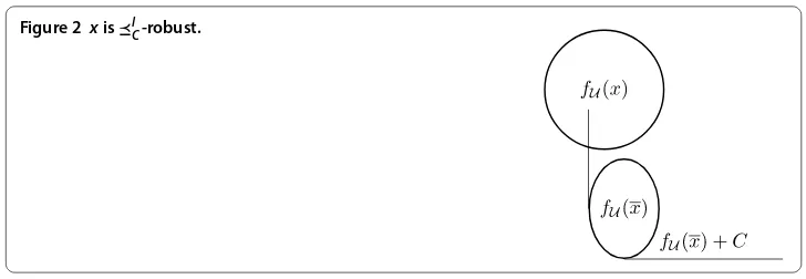
Figure 2 xisl C-robust.
whereA,B⊂Y are arbitrarily chosen sets. If we are dealing withQ=intC we suppose
intC=∅. Using this notation we derive the new concept of lQ-robustness, defined anal-ogously to uQ-robustness (Definition ).
Definition Given an uncertain multi-objective optimization problem (P(U)), a solution x∈X is called l
Q-robust if there is nox∈X\ {x}such that
fU(x) lQfUx.
The l
Q-robustness (withQ=C,Q=C\ {}andQ=intC, respectively) can be
inter-preted as an optimistic approach. The following example illustrates this concept for the caseQ=C.
Remark In Figure ,xis l
C-robust, while it is not uC-robust.
The lQ-robustness is an alternative tool for the decision maker for obtaining solutions of another type to an uncertain multi-objective optimization problem. This rather opti-mistic approach focuses on the lower bound of a setfU(x¯) for the comparison with an-other setfU(x). In particular, in the caseQ=C, a pointx∈X is called a l
C-solution
if there is no other pointx¯∈X such thatfU(x) is a subset offU(x¯) +C. Contrary to the
u
Q-robustness approach, the lQ-robustness (withQ=C,Q=C\ {}andQ=intC,
re-spectively) is hence not a worst-case concept, thus the decision maker is not considered to be risk averse but risk affine. This optimistic concept thus hedges against perturbations in the best-case scenarios.
For calculating lQ-robust solutions again the weighted sum scalarization is helpful, but in order to later on compute l
Q-robust solutions to (P(U)), we define a new weighted
sum problem in a general setting:
Lety∗∈C∗\ {}(y∗∈C#, respectively). Consider the weighted sum scalarization prob-lem
(P(U)opty∗) min
x∈Xξinf∈Uy
∗◦f(x,ξ).
Theorem Consider an uncertain multi-objective optimization problem(P(U)).The fol-lowing statements hold.
(a) Ifxis a unique optimal solution of(P(U)opt
y∗ )for somey∗∈C∗\ {},thenxis a l
C-robust solution for(P(U)).
(b) Ifxis an optimal solution of(P(U)opt
y∗)for somey∗∈C#andminξ∈Uy∗◦f(x,ξ)
exists for allx∈X,thenxis a l
(c) Ifxis an optimal solution of(P(U)opt
y∗)for somey∗∈C∗\ {}andminξ∈Uy∗◦f(x,ξ)
exists for allx∈X,thenxis a l
intC-robust solution for(P(U)).
Proof Supposexis not l
Q-robust forQ=C(Q=C\ {},Q=intC, respectively).
Con-sequently, there exists anx¯∈X\ {x}such thatf
U(x¯) +Q⊇fU(x) forQ=C(Q=C\ {}, Q=intC, respectively). That is equivalent to
∀ξ∈U∃η∈U:f(x¯,η) +Qfx,ξ
⇐⇒ ∀ξ∈U ∃η∈U:f(x¯,η)∈fx,ξ–Q. ()
Now choosey∗∈C∗\ {}forQ=C(y∗∈C#forQ=C\ {},y∗∈C∗\ {}forQ=intC,
respectively) arbitrary, but fixed. Hence, we obtain from ()
⇒ ∀ξ∈U∃η∈U:y∗◦f(x,η)≤(<, <, respectively)y∗◦fx,ξ
⇒ ∀ξ∈U:inf η∈Uy
∗◦f(x,η)≤(<, <, respectively)y∗◦fx,ξ
⇒ inf
η∈Uy
∗◦f(x,η)≤(<, <, respectively) inf ξ∈Uy
∗◦fx,ξ,
in contradiction to the assumptions.
Based on these results, we are able to present the following algorithm that computes ( lC/ lC\{}/ lintC)-robust solutions toP(U).
Algorithm Deriving ( lC / lC\{} / lintC)-robust solutions for (P(U)) based on
weighted sum scalarization:
Input & Step -: Analogous to Algorithm , only replacing (P(U)y∗) by (P(U)opty∗ ) and
replacingmaxξ∈Uy∗◦f(x,ξ)bymin
ξ∈Uy∗◦f(x,ξ).
The next algorithm computes ( lC/ lC\{}/ lintC)-robust solutions via weighted sum
scalarization by altering the weights:
Algorithm Calculating a single desired ( l
C/ lC\{}/ lintC)-robust solution for (P(U))
based on weighted sum scalarization:
Input & Step -: Analogous to Algorithm , only replacing (P(U)y¯∗) by (P(U)opt¯y∗ ),
maxξ∈Uy∗ ◦ f(x,ξ) by minξ∈Uy∗ ◦ f(x,ξ) and (P(U)y¯∗+tk+(yˆ∗–y¯∗)) by (P(U)opt¯y∗+tk+(ˆy∗–¯y∗)).
3.3 sC-Robustness
Now, we use the set less order relation sQwithQ=C,Q=C\ {}andQ=intC, respec-tively (compare Definition ) forA,B⊂Yarbitrarily chosen sets:
A sQB:⇐⇒A⊆B–QandA+Q⊇B.
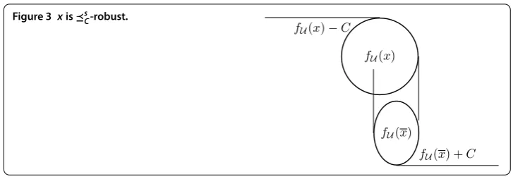
Figure 3 xissC-robust.
Definition A solutionxof (P(U)) is called ( s
C/ sC\{}/ sintC)-robust if there is no ¯
x∈X\ {x}such that
fU(x¯) sQfUx
forQ=C(Q=C\ {},Q=intC, respectively).
Remark Figure shows an element x∈X that is s
C-robust, while it is not uintC
-robust.
Remark Note that a lC-robust solution is as well sC-robust by definition. The same assertion holds for a u
C-robust solution.
The concept of sC-robustness can be interpreted in the following way: In a situation where it is not clear if one should follow a risk affine or risk averse strategy (e.g., the de-cision maker is not at hand or wants to get a feeling for the variety of the solutions) this concept might be helpful as it calculates solutions which reflect these different strategies. Therefore, this concept can serve as a pre-selection before deciding a definite strategy.
Computing s
C-robust solutions is possible with the help of the following optimization
problem:
(P(U)biobjy∗ ) h(x) :=
infξ∈Uy∗◦f(x,ξ)
supξ∈Uy∗◦f(x,ξ)
→v–min x∈X
withy∗∈C∗\ {}(y∗∈C#, respectively). For (P(U)biobj
y∗ ), we use the solution concept of
weak Pareto efficiency: An elementx∈Xis called weakly Pareto efficient for (P(U)biobj
y∗ ),
if
h(X)∩hx–intR=∅.
Furthermore, a pointx∈Xis called strictly Pareto efficient for (P(U)biobjy∗ ), if
hX\x∩hx–R=∅.
We prove the following theorem.
(a) Ifxis strictly Pareto efficient for problem(P(U)biobj
y∗ )for somey∗∈C∗\ {},thenx is sC-robust.
(b) Ifxis weakly Pareto efficient for problem(P(U)biobj
y∗ )for somey∗∈C∗\ {}and minξ∈Uy∗◦f(x,ξ)andmaxξ∈Uy∗◦f(x,ξ)exist for allx∈Xand the chosen weight
y∗∈C∗\ {},thenxis s
intC-robust.
(c) Ifxis weakly Pareto efficient for problem(P(U)biobj
y∗ )for somey∗∈C#and minξ∈Uy∗◦f(x,ξ)andmaxξ∈Uy∗◦f(x,ξ)exist for allx∈Xand the chosen weight
y∗∈C#,thenxis s
C\{}-robust.
Proof Letxbe strictly Pareto efficient (weakly Pareto efficient, weakly Pareto efficient) for problem (P(U)biobjy∗ ) with somey∗∈C∗\ {}(y∗∈C∗\ {},y∗∈C#, respectively),i.e.,
there is nox¯∈X\ {x}such that
inf ξ∈Uy
∗◦f(x,ξ)≤(<, <, respectively) inf ξ∈Uy
∗◦fx,ξand
sup ξ∈U
y∗◦f(x,ξ)≤(<, <, respectively)sup ξ∈U
y∗◦fx,ξ.
Now supposexis not ( s
C/ sintC/ sC\{})-robust. Then there exists anx¯∈X\ {x}such that
fU(x¯) +Q⊇fUxandfU(x¯)⊆fUx–Q
forQ=C(Q=intC,Q=C\ {}). That implies
∃¯x∈X\x:∀ξ,ξ∈U∃η,η∈U:f(x¯,η) +Qf
x,ξ
and
f(x¯,ξ)∈f
x,η
–Q ()
forQ=C(Q=intC,Q=C\ {}). Choose nowy∗∈C∗\ {}(y∗∈C∗\ {},y∗∈C#) as in problem (P(U)biobjy∗ ). We obtain from ()
∃¯x∈X\x:∀ξ,ξ∈U∃η,η∈U:y∗◦f(x,η)≤(<, <, respectively)y∗◦f
x,ξ
andy∗◦f(x,ξ)≤(<, <, respectively)y∗◦f
x,η
⇒inf ξ∈Uy
∗◦f(x,ξ)≤(<, <, respectively) inf ξ∈Uy
∗◦fx,ξ
andsup ξ∈Uy
∗◦f(x,ξ)≤(<, <, respectively)sup ξ∈Uy
∗◦fx,ξ.
The last two strict inequalities hold because the minimum and maximum exist. But this
is a contradiction to the assumption.
Based on these observations, we can formulate the following algorithm for computing
s
C-robust solutions toP(U).
Algorithm Computing ( s
C/ sC\{}/ sintC)-robust solutions using a family of problems
(P(U)biobjy∗ ):
Input & Step -: Analogous to Algorithm .
Step : IfSOLwe(y∗) =∅, then go to Step .
Step : Choosex¯∈SOLwe(y∗). SetSOLwe(y∗) :=SOLwe(y∗)\ {¯x}.
(a) Ifxis a strictly Pareto efficient solution of (P(U)biobjy∗ ), thenxis sC-robust for
(P(U)), thus
OptC:=OptC∪ {x}.
(b) Ifxis weakly Pareto efficient for problem (P(U)biobjy∗ ) andy∗∈C#and
minξ∈Uy∗◦f(x,ξ)andmaxξ∈Uy∗◦f(x,ξ)exist for allx∈Xand the chosen weight y∗∈C#, thenxis s
C\{}-robust for (P(U)), thus
OptC\{}:=OptC\{}∪ {x}.
(c) Ifxis a weakly Pareto efficient solution of (P(U)biobjy∗ ) andmaxξ∈Uy∗◦f(x,ξ)and
minξ∈Uy∗◦f(x,ξ)exist for allx∈X, thenxis sintC-robust for (P(U)), thus
OptintC:=OptintC ∪ {x}.
Step : Go to Step .
In the following we present an algorithm that computes s
C-robust solutions while
vary-ing the weights in the vector of objectives of problem (P(U)biobjy∗ ).
Algorithm Computing ( sC/ sC\{}/ sintC)-robust solutions using a family of
prob-lems (P(U)biobjy∗ ):
Input & Step - & Step -: Analogous to Algorithm , only replacing (P(U)¯y∗) by
(P(U)biobj¯y∗ ) and (P(U)y¯∗+tk+(ˆy∗–y¯∗)) by (P(U) biobj
¯
y∗+tk+(ˆy∗–¯y∗)). Step : Analogous to Step of Algorithm .
3.4 Alternative set less ordered robustness
Another way of combining theu- andl-type set-relations is the alternative set less order relation:
Definition (Alternative set less order relation (compare Ide and Köbis [])) LetC⊂ Y be a proper closed convex and pointed cone. Furthermore, letA,B⊂Y be arbitrarily chosen sets. Then the alternative set less order relation is defined by
A aCB:⇐⇒A uCBorA lCB.
Based on this definition we can now define the concept of aC-robustness for general cones:
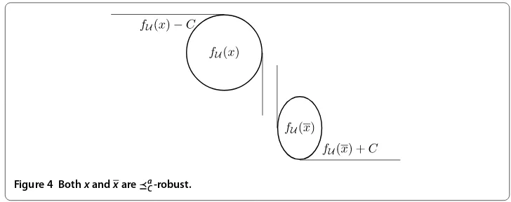
Definition A solutionxof (P(U)) is called ( a
C/ aC\{}/ aintC)-robust if there is no ¯
x∈X\ {x}such that
fU(x¯) aQfUx
Figure 4 Bothxandxarea C-robust.
The following example illustrates aC-robust solutions.
Remark In Figure , bothxandxare a
C-robust.
The next lemma follows directly from the definitions.
Lemma Note that a solution of(P(U))is a
C-robust if and only if it is lC-robust and u
C-robust.
As this lemma shows, the concept of a
C-robustness is rather restrictive as only
solu-tions which are u
C-robust and lC-robust, thus reflect both a risk averse and a risk affine
strategy, are also aC-robust. Therefore, this concept is fit for a decision maker who does not want to make any mistake in terms of the best or worst cases. We can see easily that such an approach would be very restrictive against the solutions and that only very few solutions should fulfill these conditions.
Due to this Lemma , from Algorithms and , we can deduce the following algorithm for calculating aC-robust solutions to (P(U)).
Algorithm Deriving ( aC/ aC\{}/ aintC)-robust solutions to (P(U)):
Input: Uncertain multi-objective problem (P(U)), solution sets OptCa = OptaC\{} =
OptaintC=∅.
Step : Compute a set of( l
C/ lintC/ lC\{})-robust solutions(OptlC,OptlintC,OptlC\{})
us-ing Algorithm or . Step : Compute a set of( u
C/ uintC/ uC\{})-robust solutions(OptuC,OptuintC,OptuC\{})
us-ing Algorithm or .
Output: Set of( a
C/ aintC/ aC\{})-robust solutions
OptaC=OptuC∩OptlC,
OptaintC=OptuintC∩OptlintC,
OptaC\{}=OptuC\{}∩OptlC\{}.
3.5 Further relationships between the concepts
Figure 5 xissC-robust, but neitheruC-robust nor l
C-robust.
Figure 6 Scheme of solutions to an uncertain multi-objective optimization problem.
We summarize the relationship between the various robustness concepts in Figure .
4 Conclusions
In the following we will explain that our algorithms presented in Section can be used for solving special classes of set-valued optimization problems.
Having a close look at all the concepts of robustness from Section , we can see that in fact all of these are set-valued optimization problems.
Consider a set-valued optimization problem of the form
(SP– ) -minimizeF(x), subject tox∈X,
with some given preorder and a set-valued objective mapF:X⇒Y, we can see the following.
If the preorder is given by l
C, uC, or sC with some proper closed convex pointed
coneC⊂Y andF(x) can be parametrized by parametersξ ∈U with some setU in the way that
F(x) :=fU(x) for allx∈X,
We revealed strong connections between set-valued optimization and uncertain multi-objective optimization. Furthermore, we derived our results in a more general setting than in [] and []. In particular, we provided solution algorithms for a certain class of set-valued optimization problems. It seems possible to extend this class of problems to a more general one, but this is future work and of interest for the next steps in this area of research. Moreover, this paper makes very clear that finding robust solutions to uncertain multi-objective optimization problems can be interpreted as an application of set-valued opti-mization. Thus, robust solutions to uncertain multi-objective optimization problems can be obtained by using the solution techniques from set-valued optimization. Formulating concrete algorithms of this kind is another topic for future research.
Competing interests
The authors declare that they have no competing interests.
Authors’ contributions
All authors contributed equally to the writing of this paper. All authors read and approved the final manuscript.
Author details
1University Göttingen, Göttingen, Germany.2University Erlangen-Nürnberg, Bavaria, Germany.3Shimane University,
Hamada, Shimane, Japan.4Martin-Luther-University Halle-Wittenberg, Halle, Germany.
Acknowledgements
Supported by DFG RTG 1703 ‘Resource Efficiency in Interorganizational Networks’.
Received: 30 September 2013 Accepted: 14 March 2014 Published:31 Mar 2014
References
1. Stewart, T, Bandte, O, Braun, H, Chakraborti, N, Ehrgott, M, Göbelt, M, Jin, Y, Nakayama, H, Poles, S, Di Stefano, D: Real-world applications of multiobjective optimization. In: Branke, J, Deb, K, Miettinen, K, Slowinski, R (eds.) Multiobjective Optimization: Interactive and Evolutionary Approaches. Lecture Notes in Computer Science, vol. 5252, pp. 285-327. Springer, Berlin (2008)
2. Scott, EM, Saltelli, A, Sörensen, T: Practical experience in applying sensitivity and uncertainty analysis. In: Sensitivity Analysis. Wiley Ser. Probab. Stat., pp. 267-274. Wiley, Chichester (2000)
3. Birge, JR, Louveaux, FV: Introduction to Stochastic Programming. Springer, New York (1997)
4. Kouvelis, P, Yu, G: Robust Discrete Optimization and Its Applications. Kluwer Academic, Dordrecht (1997) 5. Ben-Tal, A, El Ghaoui, L, Nemirovski, A: Robust Optimization. Princeton University Press, Princeton (2009)
6. Fischetti, M, Monaci, M: Light robustness. In: Ahuja, RK, Moehring, R, Zaroliagis, C (eds.) Robust and Online Large-Scale Optimization. Lecture Notes in Computer Science, vol. 5868, pp. 61-84. Springer, Berlin (2009)
7. Liebchen, C, Lübbecke, M, Möhring, RH, Stiller, S: The concept of recoverable robustness, linear programming recovery, and railway applications. In: Ahuja, RK, Möhring, RH, Zaroliagis, CD (eds.) Robust and Online Large-Scale Optimization. Lecture Note on Computer Science, vol. 5868. Springer, Berlin (2009)
8. Klamroth, K, Köbis, E, Schöbel, A, Tammer, C: A unified approach for different concepts of robustness and stochastic programming via nonlinear scalarizing functionals. Optimization62, 649-671 (2013)
9. Goerigk, M, Schöbel, A: A scenario-based approach for robust linear optimization. In: Proceedings of the 1st International ICST Conference on Practice and Theory of Algorithms in (Computer) Systems (TAPAS). Lecture Notes in Computer Science, pp. 139-150. Springer, Berlin (2011)
10. Soyster, AL: Convex programming with set-inclusive constraints and applications to inexact linear programming. Oper. Res.21, 1154-1157 (1973)
11. Ben-Tal, A, Nemirovski, A: Robust convex optimization. Math. Oper. Res.23(4), 769-805 (1998)
12. Deb, K, Gupta, H: Introducing robustness in multi-objective optimization. Evol. Comput.14(4), 463-494 (2006) 13. Branke, J: Creating robust solutions by means of evolutionary algorithms. In: Eiben, EA, Bäck, T, Schenauer, M,
Schwefel, H-P (eds.) Parallel Problem Solving from Nature - PPSNV. Lecture Notes in Computer Science, vol. 1498, pp. 119-128. Springer, Berlin (1998)
14. Barrico, C, Antunes, CH: Robustness analysis in multi-objective optimization using a degree of robustness concept. In: IEEE Congress on Evolutionary Computation. CEC 2006, pp. 1887-1892 (2006)
15. Steponaviˇc˙e, I, Miettinen, K: Survey on multiobjective robustness for simulation-based optimization. Talk at the 21st International Symposium on Mathematical Programming, August 19-24 2012, Berlin, Germany (2012)
16. Witting, K: Numerical algorithms for the treatment of parametric multiobjective optimization problems and applications. PhD thesis, Universität Paderborn, Paderborn (2012)
17. Kuroiwa, D, Lee, GM: On robust multiobjective optimization. Vietnam J. Math.40(2-3), 305-317 (2012)
18. Ehrgott, M, Ide, J, Schöbel, A: Minmax robustness for multi-objective optimization problems. Eur. J. Oper. Res. (2014). doi:10.1016/j.ejor.2014.03.013
19. Kuroiwa, D, Lee, GM: On robust convex multiobjective optimization. J. Nonlinear Convex Anal. (2013, accepted) 20. Eichfelder, G, Jahn, J: Vector optimization problems and their solution concepts. In: Recent Developments in Vector
21. Kuroiwa, D: Some duality theorems of set-valued optimization with natural criteria. In: Proceedings of the International Conference on Nonlinear Analysis and Convex Analysis, pp. 221-228. World Scientific, Singapore (1999) 22. Kuroiwa, D: The natural criteria in set-valued optimization. S ¯urikaisekikenky ¯usho K ¯oky ¯uroku1031, 85-90 (1998).
Research on nonlinear analysis and convex analysis (Kyoto, 1997)
23. Nishnianidze, ZG: Fixed points of monotone multivalued operators. Soobshch. Akad. Nauk Gruzin. SSR114(3), 489-491 (1984)
24. Young, RC: The algebra of many-valued quantities. Math. Ann.104(1), 260-290 (1931)
25. Takahashi, W: Nonlinear Functional Analysis. Fixed Point Theory and Its Applications. Yokohama Publishers, Yokohama (2000)
26. Takahashi, W: Introduction to Nonlinear and Convex Analysis. Yokohama Publishers, Yokohama (2009) 27. Aoyama, K, Kohsaka, F, Takahashi, W: Proximal point methods for monotone operators in Banach spaces. Taiwan.
J. Math.15(1), 259-281 (2011)
28. Takahashi, W: Nonlinear mappings in equilibrium problems and an open problem in fixed point theory. In: Fixed Point Theory and Its Applications, pp. 177-197. Yokohama Publishers, Yokohama (2010)
29. Ide, J, Köbis, E: Concepts of robustness for multi-objective optimization problems based on set order relations (2013) 30. Kuroiwa, D: On set-valued optimization. Nonlinear Anal.47(2), 1395-1400 (2001)
31. Jahn, J, Ha, TXD: New order relations in set optimization. J. Optim. Theory Appl.148(2), 209-236 (2011) 32. Kuroiwa, D: Existence theorems of set optimization with set-valued maps. J. Inf. Optim. Sci.24(1), 73-84 (2003) 33. Ehrgott, M: Multicriteria Optimization, 2nd edn. Springer, Berlin (2005)
34. Göpfert, A, Riahi, H, Tammer, C, Z˘alinescu, C: Variational Methods in Partially Ordered Spaces. Springer, New York (2003)
10.1186/1687-1812-2014-83