O R I G I N A L R E S E A R C H
Open Access
A gamma-distribution convolution model
of
99m
Tc-MIBI thyroid time-activity curves
Carl A. Wesolowski
1,2*, Surajith N. Wanasundara
1, Michal J. Wesolowski
1, Belkis Erbas
3and Paul S. Babyn
1* Correspondence: [email protected] 1Department of Medical Imaging,
Royal University Hospital, College of Medicine, University of
Saskatchewan, 103 Hospital Drive, Saskatoon, SK S7N 0W8, Canada 2
Nuclear Medicine, Department of Radiology, Faculty of Medicine, Memorial University of Newfoundland, 300 Prince Philip Drive, St. John’s, NL A1B 3X7, Canada
Full list of author information is available at the end of the article
Abstract
Background:The convolution approach to thyroid time-activity curve (TAC) data fitting with a gamma distribution convolution (GDC) TAC model following bolus intravenous injection is presented and applied to99mTc-MIBI data. The GDC model is a convolution of two gamma distribution functions that simultaneously models the distribution and washout kinetics of the radiotracer.
The GDC model was fitted to thyroid region of interest (ROI) TAC data from 1 min per frame99mTc-MIBI image series for 90 min; GDC models were generated for three patients having left and right thyroid lobe and total thyroid ROIs, and were contrasted with washout-only models, i.e., less complete models. GDC model accuracy was tested using 10 Monte Carlo simulations for each clinical ROI.
Results:The nine clinical GDC models, obtained from least counting error of counting, exhibited corrected (for 6 parameters) fit errors ranging from 0.998% to 1.82%. The range of all thyroid mean residence times (MRTs) was 212 to 699 min, which from noise injected simulations of each case had an average coefficient of variation of 0.7% and a not statistically significant accuracy error of 0.5% (p= 0.5, 2-sample pairedttest). The slowest MRT value (699 min) was from a single thyroid lobe with a tissue diagnosed parathyroid adenoma also seen on scanning as retained marker. The two total thyroid ROIs without substantial pathology had MRT values of 278 and 350 min overlapping a published99mTc-MIBI thyroid MRT value. One combined value and four unrelated washout-only models were tested and exhibited R-squared values for MRT with the GDC, i.e., a more complete concentration model, ranging from 0.0183 to 0.9395.
Conclusions:The GDC models had a small enough TAC noise-image misregistration (0.8%) that they have a plausible use as simulations of thyroid activity for querying performance of other models such as washout models, for altered ROI size, noise, administered dose, and image framing rates. Indeed, of the four washout-only models tested, no single model approached the apparent accuracy of the GDC model using only 90 min of data. Ninety minutes is a long gamma-camera acquisition time for a patient, but a short a time for most kinetic models. Consequently, the results should be regarded as preliminary.
Keywords:Gamma distribution convolution,99mTc-hexakis-methoxy-isobutyl-isonitrile, Thyroid, Time-activity curve, Gamma camera
Background
The use of technetium-99m hexakis-methoxy-isobutyl-isonitrile (99mTc-MIBI) as a
thyroid and parathyroid imaging agent was first proposed in the late 1980s [1]. Since its inception, 99mTc-MIBI scintigraphy has been shown to be more accurate and sensitive than comparable imaging techniques and is currently used to detect and localize differen-tiated thyroid cancer [2, 3], parathyroid adenoma [1, 4], parathyroid hyperplasia [5, 6], and parathyroid carcinoma [4, 7].
Several 99mTc-MIBI image acquisition protocols and analysis techniques have been devised over the last quarter century to aid in the detection of abnormal thyroid and parathyroid tissue, these include dual-phase scintigraphy [8], factor analysis of a dynamic scan [9], and time-activity curve (TAC) analysis of a dynamic scan [10]. TAC analysis provides a means of differentiating between normal and abnormal tissues by comparing of radiotracer uptake and washout in different regions of interest (ROIs).99mTc-MIBI does not undergo significant chemical changes in the body and therefore is passively taken up in the thyroid and parathyroid tissues and is cleared rapidly from the blood [11]. TAC analysis also has the potential to provide detailed pharmacokinetic information from ROIs. Pharmacokinetic parameters, such as the tracer mean residence time (MRT) and elimination half-life can be used to quantify and characterize disease states, which ultimately may aid in the diagnosis of thyroid and parathyroid disease.
It is a common practice to inject a bolus of a drug into a vein, but to take images or venous samples elsewhere. Before the time of first arrival of activity in the sampling re-gion, there is no drug and no signal in that remote site. Most pharmacokinetic bolus models ignore this initial mixing and are washout-only models having a maximum amplitude initially. Thus, at the earliest times following a bolus, there is a severe mis-match between a washout model and the signal it models. Consequently, most of the routinely used pharmacokinetic models, e.g., classic compartmental washout models, do a poor job of fitting early-time organ activity [12, 13]. Thus, washout functions do not fit concentration or time-activity curves well enough to serve as accurate simula-tion study models. To model the entire TAC accurately, it is necessary to use a math-ematical model that includes at least some of the drug arrival and organ drug distribution effects. Convolutions of two functions as an impulse response model can approximate the entire TAC accurately [14, 15]. Of these two functions, the first or fast function can be thought of as an organ feed or stimulus function consisting of rapidly changing blood pool background within the organ. The second can be thought of as the response or result of bathing the parenchyma of an organ with drug [16, 17].
While there has been some work on the biodistribution and pharmacokinetics of
99m
functions, a closed form convolution is self-contained and thus useful as a surrogate for otherwise impossible to perform exhaustive testing while still maintaining a degree of realism.
In this context, we aim to demonstrate that following a peripheral intravenous bolus injection, the thyroid has a TAC that can be modelled accurately using the closed form convolution of two gamma distribution (GD) functions. The first GD of the GDC approximates thyroid gland marker arrival and distribution, and the second GD, the
thyroid marker washout. We apply this model to TAC’s from dynamic 99mTc-MIBI
scans, and show how it can be used to calculate organ statistics, especially MRT values. Next, we perform a surrogate test example, Monte Carlo simulation of self-consistency of the GDC algorithm to check the accuracy of modelling. Finally, we compare the GDC, a more complete model of concentration, to four of the best available washout-only models for our 90-minute data.
Theory
A convolution of two random variables can be used to form an impulse response model of time activity of an imaged organ’s radioactivity [14]. The first, fastest random variable is the impulse or blood pool that feeds the organ, and the second, slower random variable is the washout of activity from that organ. Note (1) that random variables are modelled as density functions and add by convolution, (2) that the total area of any density function is one, and (3) that any convolution of density functions is itself a density function with a total area of one [23, 24]. Closed form convolutions that model both arrival and washout have also long been used as pharmacokinetics models as originally inspired by Bateman’s treatment of radioactive density functions of parent (be−bt) and daughter species (βe−βt) [25]. This latter is perhaps best written as the exponential density function convolution (EDC)
EDCðb;β;tÞ ¼be−bt⊗βe−βt
¼
g
bβe−βtb−−βe−bt; b≠β
b2t e−bt ; b¼β t≥0
0 gt<0
:
8 > > < > >
: ð1Þ
The amount of daughter (or time activity) at time zero, i.e., the initial EDC func-tional height, is zero in this particular non-negative-valued Bateman equation. However, when taken out of the parent-daughter decay context, Eq. (1) becomes only approximate. Generally, whatever an exponential distribution (ED) can model is typically better modelled by a gamma distribution (GD) [26]. Exponential distri-butions are not the preferred shapes to explain organ bolus input function shapes,
for which GDs or other functions are more useful [27–29]. To model the
to the contrary [34], GDs do not derive from serial EDCs. Rather, Eq. (1) is a special case GD convolution–see the text following Eq. (5), and a derivation of the GD appears elsewhere [35].
The arrival of the99mTc-MIBI within the thyroid is not instantaneous. The fast signal or blood-pool activity within the thyroid is approximated here using a gamma distribu-tion (GDfast) density function that for timet (min) is time-offset bytΑ('A' for arrival)
and zero beforetΑby lettingτ=t−tA, and setting
GDfastða; b; τÞ ¼ ba
Γð Þa τ
a−1e−bτ; τ≥0
0 ; τ<0
;
8 < :
ð2Þ
where, if the dimensionless shape parameter a > 1 would yield a skewed bell curve and if a < 1 a decaying saw tooth or spike, and where b is the rate scalar (per min).
Washout functions are the impulse response to an instantaneously distributed signal and strictly washout. A washout function can be modelled as a gamma distribution,
GDWOðα;β;τÞ ¼
βα
Γð Þα τ
α−1e−β τ; τ≥0
0 ; τ<0
;
8 < :
ð3Þ
where α < 1 is the shape parameter condition for washout, i.e., a monotonic decrease of functional height in time. Next, the GDC model is created by convolving GDfastand GDWO,
GDC að ;b;α;β;τÞ ¼GDfastða;b;τÞ⊗GDWOðα;β;τÞ; ð4Þ
Substitution of Eqs. (1) and (2) into Eq. (4) leads to
GDC að ;b;α;β;τÞ ¼
baβα
ΓðaþαÞe
−bττaþα−1
1F1½α;aþα;ðb−βÞτ; τ>0
0 ; τ≤0
;
8 > < >
: ð5Þ
which is a density function consisting of a gamma variate multiplied by 1F1(A; B; Z), where the latter is a confluent hypergeometric function of the first kind1[36,37]. For a = 1 and α= 1, Eq. (5) reduces to Eq. (1), which in turn demonstrates that Eq. (5) is more general than Eq. (1). That is, in practice, the GDC would reduce to a Bateman density if a = 1 andα= 1 were plausible parameter values. For b =β, Eq. (5) reduces to GD(a +α, b;τ), a statistically implausible simplification used nonetheless [34]. Although serial GD convolution is known [20, 26], the easily recognizable simple closed form for the two GD convolution of Eq. (5) is a recent development [see [20], Eq. (2)].
Mean residence time, MRT, is independent of any TAC scaling, and its value can be calculated directly from a density function,f(t), as follows:
MRT¼
Z ∞
0
t f tð Þdt: ð6Þ
MRTGDC→tAþMRTfastþMRTWO¼tAþ a bþ
α
β: ð7Þ
However, tracer residencewithinthe thyroid starts at the time of tracer first arrival within that organ, such thattAis unrelated to thyroid residence time. Moreover, MRTfast ¼ab
quantifies the delivery and uptake of tracer in the thyroid, and only MRTWO¼αβ
relates to how the thyroid washes out of tracer activity once that activity is distributed within the thyroid. That is, MRTWOcharacterizes the response of thyroid tissue to an
instantaneous signal.
Methods
Patient population
The data from three patients were acquired at the Hacettepe University Medical School and were processed blindly at the University of Saskatchewan. The99mTc dosages were 740 MBq. Patients 1 and 3 underwent 99mTc-MIBI scanning for metastatic screening, and were negative. Patient 2 underwent parathyroid scanning for chemical hyperpara-thyroidism. On scanning, there was99mTc-MIBI retention in the lower part of the right thyroid lobe ROI found on histological examination to be a parathyroid adenoma measuring 11 × 11 mm. The GDC curve analysis was performed blindly and without knowledge of the region drawing, the scanned images, or the clinical presentation and results. Clinical correlation was performed only after the quantitative GDC results were obtained.
Data processing
Following a peripheral intravenous bolus injection, 89 one-minute per frame dynamic
99m
Tc-MIBI gamma camera images were obtained. Regions of interest (ROIs) were drawn over the right and left thyroid lobe in each frame, and the regional counts per minute were then used to construct time-activity curves (TACs). The TACs were then least Poisson noise model fit with the decay simulated GDC model, Eq. (5)—see the Appendix section—in a separate institution using Mathematica 10.3 programs using an algorithm stop condition of a 10-20 relative difference between successive iterations. Caution was taken to find global minima by including reasonable initial parameter range, starting values, but there is no absolute guarantee that global minima will be found with the Nelder-Mead (simplex) regression used. Poisson model noise cal-culations, regression fitting for Poisson models, corrected fit error quantification,
and an algorithm for finding TAC starting-time values, tA, can be found in the
Appendix section.
Time-activity curve simulations
compensate for the lack of injected misregistration by increasing the noise to larger levels due to generating Poisson model noise from larger, not decay-diminished signals (2) crosscheck the accuracy of the decay-corrected GDC model used for the clinical cases, (3) simulate drug assay when decay is not a factor, and (4) provide an example of how simulations studies can be used to model variations of experimental conditions and validate techniques.
Washout model analysis with comparison to GDC models
Comparisons of GDC MRTWOresults were made to four washout models; two different
regression methods of fitting biexponentials, and two different regression methods of fitting single gamma variates. One of these latter, Tk-GV; the Tikhonov regularized gamma variate herein adaptively minimizes the relative error of βor alternatively the minimum relative error of plasma clearance [12, 13, 32]. Briefly, Tk-GV is an approximate inverse solution to Eq. (4). That is forC(t) = GDfastTk-GVWO, then Tk-GVWO= GDfast(−1)⊗C(t), and Tk-GV fits
an inverse (virtual) function, not concentration itself,C(t).
Results
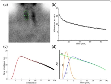
A representative example of a 99mTc-MIBI scintigram from a right thyroid lobe ROI is shown in Fig. 1a, while the corresponding TAC for the entire dynamic scan is shown in Fig. 1b. Figure 1c shows the same TAC with time on a logarithmic scale to display the rapidly changing curve at early times. Superimposed is the fit of the gamma distribution convolution (GDC) scaled (S) to the TAC. Figure 1d shows graphical representations of the fast vascular gamma distribution (GDfast), the washout gamma distribution (GDWO)
and GDC; the convolution of GDfastand GDWO.
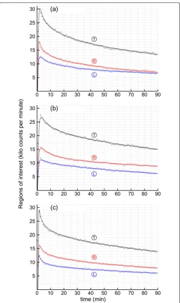
Figure 2 shows the data and fits of the GDC for all nine TAC’s for the three patients. The parameter values obtained from fitting the GDC to the TACs and the GDC fit errors are summarized below in Table 1. The GDC parameters from Table 1 were used to calculate mean residence times (MRT) for the thyroid ROIs shown in Table 2. Note in Table 2 that the GDfast, a.k.a., thyroid vascular mixing times, the MRTfast values,
averaged only 0.807 min or 0.2% of the 367.4 min MRTWO, i.e., washout times. MRTfastis
the ratio of the 'a' and b values in Table 1, and is stable even though the shapes ('a' values) of the GDfast distributions are quite variable due to the 'a' and b values
being highly correlated (r= 0.99935). The MRTWO values ranged from 211.6 to
699.0 min. Note that the left lobe, case 2L in Table 2, had the shortest MRT of
only 211.6 min, whereas the same patient’s right lobe, 2R, had the longest MRT
value, 699.0 min.
GDC parameters to the noise injected recovered parameters allowed for an independ-ent (if simplistic) measure of accuracy and precision of recovery of the parameters as listed in Table 3. The recoveries of the start times for simulation, tA, averaged an
insignificant 0.035% error (p= 0.98) suggesting that the start time algorithm of the Ap-pendix section, Eq. (12), functioned adequately. The mean decay corrected thyroid washout MRT values went from 367.4 min from the 9 clinical regressions to 369.1 min from the average of 90 simulations for an absolute error of 0.46%. Note in Table 3 that none of the GDC simulation MRT values or other parameters (apart from the fit errors mentioned above) were significantly different from their corresponding clinical parameter values. Finally, α-shape values were never close to one in the 99 simula-tions and clinical cases (absolute range from 0.8528 to 0.9445), such that the use of EDWO=βe−βt in the Bateman Eq. (1) above rather than GDWO would introduce
severe non-linear misregistration into the data fitting.
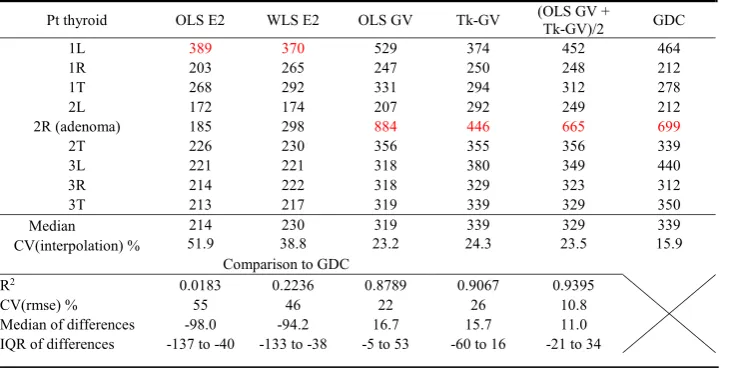
From the preceding, the 90 min of data may be sufficient for obtaining a complete concentration model, the GDC. Next, we tested to see if 90 min was a long enough time to obtain stable washout-only model MRT values. Table 4 shows a comparison of the 1st through 89th minute TAC GDC models with 5th through 89th minute TAC washout models. Two of the four 5th through 89th minute washout models are
Fig. 1Thetop left panel(a), shows a region of interest (ROI) drawn over a right thyroid lobe of an example one-minute image from a99mTc-MIBI gamma camera image sequence. Thetop right panel(b) shows the ROIs time-activity curve (TAC). Panel (c) shows the same right thyroid lobe TAC as in panel (b) with time on a logarithmic scale to better display the rapidly changing curve at early times. Superimposed is the fit of a gamma distribution convolution (GDC,solid red line) scaled to the TAC showing a good fit to the TAC (open circles). Panel (d) shows graphical representations of the GDfast, the fast vascular gamma distribution (F,orange);GDWO,
the washout gamma distribution (W,green) and the GDC; the convolution of GDfastand GDWO(G,blue). For clarity,
the vertical axis has an arbitrary scale to superimpose the GDfastfunction with the other two functions on one
ordinary least square (OLS) models; biexponential OLS E2 and gamma variate OLS GV. The other two models are not concentration models. Those are 1/C(t)2 weighted least squares E2, and the Tk-GV model minimized for least relative error ofβ; WLS E2 and Tk-GV. For each method, how well the L and R MRT values produced interpolated total thyroid MRT values was calculated as a coefficient of variation as shown in Table 4. These CV(interpolation) varied from a high value of 51.9% for OLS E2 to a low value of 15.9% for GDC. Note that due to patient variation a CV(interpolation) of zero is not expected. The MRTWOvalues for OLS E2 were of significantly shorter
dur-ation than those from the GDC model (Wilcoxon,p= 0.004).
As can be seen in Table 4, the smallest and only statistically not significant R2value
(0.0183, p= 0.7) was between OLS E2 and GDC. The parathyroid adenoma (2R) was
not identified by its MRTWOusing OLS E2 and WLS E2, but was the longest MRTWO
for all of the GV-based models and for the GDC model. Although the GV washout models; OLS GV, Tk-GV, and the average of OLS GV and Tk-GV were superior to E2 models for the single-case lesion detection, the highest R2 value with the GDC of
0.9395 for those washout models occurred for the average MRTWOvalues of OLS GV
and Tk-GV. This averaged model MRTWOvalue corresponded to a 10.8% coefficient of Table 1Parameters for the GDC fit model
Pt thyroida tA(min) a b (min− 1
) α β(min−1) S(106cts)b Fit err %c Noise % 1−R2(%)d
1L 0.195 0.846 0.909 0.8577 0.001849 3.529 1.713 1.174 0.534
1R 0.334 3.733 5.211 0.8661 0.004081 2.319 1.914 1.094 0.350
1T 0.277 1.631 2.060 0.8645 0.003106 5.222 1.421 0.800 0.271
2L 0.340 1.351 1.692 0.9408 0.004445 2.027 1.690 1.183 0.630
2R 0.282 0.995 0.928 0.8668 0.001240 6.510 1.353 1.022 0.395
2T 0.307 1.127 1.203 0.8998 0.002652 6.625 1.019 0.773 0.239
3L 0.306 7.878 11.644 0.8918 0.002029 3.201 1.801 1.225 0.818
3R 0.425 3.082 4.520 0.8942 0.002863 3.296 1.026 1.060 0.189
3T 0.374 6.470 9.842 0.8947 0.002554 6.287 0.988 0.801 0.224
a
Patient numbers 1,2,3 plus L left thyroid lobe, R right thyroid lobe, T total thyroid TACs, e.g., 1L, 2L b
Sis the scale factor used to equate AUCTAC=SAUCGDC. The AUC of the GDC is one, as it is for all density functions. The AUC of a TAC is the total counts collected in the ROI from time is zero to infinity
c
The fit error was increased to offset for the effect of using 6 fit parameters in the GDC model—see Eq. (10) d
From correlation of the TAC with the GDC model for the 89 one-minute sample times
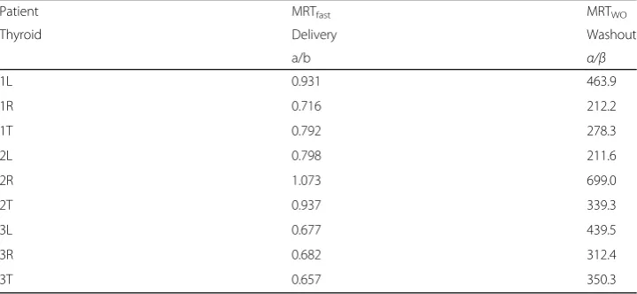
Table 2Decay-corrected MRT values in min for thyroid delivery and washout from 9 GDC models
Patient MRTfast MRTWO
Thyroid Delivery Washout
a/b α/β
1L 0.931 463.9
1R 0.716 212.2
1T 0.792 278.3
2L 0.798 211.6
2R 1.073 699.0
2T 0.937 339.3
3L 0.677 439.5
3R 0.682 312.4
variation of root mean square error, CV(rmse), agreement with GDC MRTWO. This
compares to the Monte Carlo testing of the GDC MRTWO, with a 0.69% (CV) for
pre-cision and 0.46% for accuracy—see Table 3.
For the results listed, we processed the TACs as supplied. These neither represented the values for single thyroid lobes nor for whole thyroid glands but rather a mixture of
Table 3Poisson noise simulations and accuracy of recovery of generating parameters following regression
Parameters tA a b α β Sa MRTWO
Units min none min−1 none min−1 106counts min
Clinical mean values 0.316 3.013 4.223 0.8863 0.00276 4.335 367.4
Simulation mean valuesb 0.316 3.314 4.588 0.8859 0.00275 4.342 369.1
Units Percentage (%)
Mean simulation CV errorc 2.4 0.23 1.6 0.26 3.1 2.6 0.69
Absolute error in percentd 0.035 10.0 8.6 −0.038 −0.38 0.15 0.46
Units Probability
Probability of no differencee 0.98 0.44 0.52 0.32 0.38 0.73 0.51
a
The scale factorsS, used to scale GDC, are the total counts collected in the ROI from time is zero to infinity b
Each set of clinical parameters for 9 cases was used to generate 10 different noisy data sets. The simulation mean values are from all 90 simulations
c
This is the mean value of 9 coefficients of variation (CV), where each CV is from 10 simulations d
Error is 100 times mean simulation minus clinical values divided by mean clinical value time e
No significant differences to the 0.05 level from two-tailedttests for zero difference between 9 paired samples using mean values of 10 simulations for each clinical result and the clinical parameter results themselves
Table 4Mean residence time (MRTWOin minutes) results for simple washout models fit from the
5th to 89th minute ROIs and compared to the gamma distribution convolution (GDC) MRTWOof
the texta
a
Regressions used were ordinary least squares (OLS), weighted least squares [WLS; 1/C(t)2weighting], and an inverse method; Tk-GV. These were applied to biexponential (E2) and gamma variate (GV) functions. The longest MRT value for each method is in red. IQR is interquartile range. How well the total (T) thyroid interpolated the L and R MRT values was calculated as a coefficient of variation of interpolation, CV(interpolation), from the standard deviation of the distances to interpolation,d= MRTTotal− min{MRTL, MRTR}, divided by the mean of their interpolation interval,ii= |MRTL−MRTR|. The CV of the root mean square error
CV(rmse) was calculated for methodM≠MRTGDCas
Xn
i¼1
MRTMð Þi−MRTGDCð Þi
½ 2
n
( )1
2 Xn
i¼1 MRTGDCð Þi
n
" #−1
. The median of
those values. For GDC models of whole thyroid glands listed in Table 4, the IQR of MRT values was 72 min. The GDC IQR from the given mixture of regions was 206 min, and for thyroid lobes without whole thyroid MRT values, the IQR value was 311 min (via Excel PERCENTILE.EXC subtraction or equivalent algorithm).
Discussion
The quality of the fit results illustrated in Fig. 2 and listed in Table 1 suggest that gamma distribution convolutions, GCDs, can be used to form scaled models that
accurately follow TACs of 99mTc-MIBI activity in the thyroid. A GDC implies two
gamma distributions, GDs: a GDfast delivery to the thyroid function and a slower
GDWO washout from the thyroid function. Note that these separate gamma
distribu-tions were not observed directly, but rather were implied by the thyroid ROI data and the GDC fitting parameters. To illustrate these behaviours, the individual GDfast,
GDWO, and GDC density functions are displayed in Fig. 1d. That figure shows that the
effect of the GDfaston the GDC dissipated in time, so that eventually the GDWOcurve
converges to the path of the data (after ~1 hr). This, and the results in Table 4, confirm that washout-only models are only indirectly related to TAC or concentration models [14, 15], and that, in turn explains why washout models appear to require more extended time-sampling than the GDC model. For example, the GDC residuals were homoscedastic over the entire sampling space, which is never the case for washout-only models as wash-out models are at a maximum value initially, when actual concentration is zero. It has been shown in other systems that washout models, even with a 10 min start time, statisti-cally significantly mismatched early data and agreed better with late data [12].
Most pharmacokinetic models are thought of as successful when their curve fit errors average 10% or less [as rmse in 38]. More important than curve fitting error is how precise the models are for the parameter of interest, or in our case,
MRTWO.We note that no washout model for predicting GDC MRTWOhad less than a
10% precision error measured as CV(rmse)—see Table 4—to unequivocally suggest its
use with only 90 min of99mTc-MIBI data. The average MRTWOfor OLS GV and Tk-GV
correlated best to GDC MRTWO. The OLS GV is a direct fit to concentration and Tk-GV
is an inverse solution, virtual concentration fit, and which methods have errors in opposite directions when applied to only 90 min of data. This combined MRT measurement had an error of 10.8% compared to the GDC model, i.e., it was almost good enough for clinical use. Thus, the GDC model may find use as a standard for investigating simpler washout models. Herein, each OLS model (OLS E2 and OLS GV) was outperformed for
MRTWOR2with GDC by its corresponding weighted alternative; WLS E2 and Tk-GV.
Alone amongst the methods tested, MRTWOOLS E2 did not (statistically significantly)
regress or correlate to MRTWOGDC (or to Tk-GV). Better correlated was WLS E2. The
1/C(t)2least squares weighting fits biexponential washout models favour fitting the later data to obtain more accurate half-lives [39]. Although some researchers have, without much discussion, used WLS E2 rather than OLS E2 in their patient series [13, 40, 41], direct numerical evidence of improved correlation against better or more complete models, such as that in Table 4, is currently limited. From the Monte Carlo testing—see Table 3—the
GDC MRTWOhad a 0.69% (CV) precision and 0.46% accuracy, so that comparison to
No area normalized background subtraction using a second ROI outside of the thyroid ROI was performed for our analysis. For the current work, background was considered to be the blood pooling within the thyroid region as modelled by the fast or delivery function activity, whose short time-duration (MRTfast in Table 2) agrees in a
general way with the short time that99mTc-MIBI is known to remain in the blood [11]. The background adjustment herein was to treat the blood pooling in the thyroid ROI as the delivery vehicle to the extravascular tissue within the same ROI for later washout. This is similar to the fast decaying quasi-exponential functional treatment of background for 99mTc-MAG3 renal scintigraphy by the recently developed blood-pool compensation and modified Patlak-Rutland methods both of which do not use classical background regions [17, 42–44]. The shape of the fast curve, GDfast, i.e., the individual
'a' values in Table 1 were variable and implied shapes sometimes heavier tailed than exponential distributions (a < 1), and sometimes lighter-tailed, i.e., closer to normal distributions (a > 1). It would be remiss to imply that the GDfast curve shape is
accurately captured, i.e., the GDfastshape coefficient, 'a' was quite variable—see Table 1.
The difficulty in quantifying the GDfastshape is likely due to the unavoidable sparseness
of nuclear decay data. Using faster framing rates to capture the shape of the fast function better would likely increase both misregistration and noise as these measures covaried (r= 0.77 see Misregistration in the Appendix section). However, the mean MRTfast times from patient studies, numerically a/b, were quite stable as the 'a' and b
values were highly correlated (r= 0.99934). From the simulations, the mean standard deviation MRTfast time was only 1.0 s (within cases), where the population standard
deviation (between cases) was 0.137 min (8.2 s) suggesting that two parameter GDfast
functions are adequate for calculating MRTfast values. The washout function, GDWO,
has a shape parameter, α< 1, which yields a curve that is monotonically decreasing (washing out), with very stable shapes herein [CV(α) = 2.9% from patient studies, 2.6% from simulations between cases, and 0.26% from simulations within cases]. The rate scalar (β) of the GDWOis much smaller (i.e., slower) than the rate scalar (b) of the fast
curve. Combined with concentration curves, washout models are used for predicting clearance, as they conserve mass. However, washout models do not form accurate models of early time TACs—see Fig. 1d—and [45], and that is a good motive for creat-ing more complete models, i.e., that better fit the data, with the alternatives becreat-ing (1) to ignore the early data, extend the data collection for hours, and to use models whose misregistration magnifies substantially outside of fit range—see [12, 45], or (2) include the early data and suffer significant, large misregistration within the fit range—see [12]. Despite the pleomorphic shapes of an assumed fast function, and the noise problem, the resulting GDC functions’misregistration of the TACs counts was only 0.80% with a total fit error of 1.44% (seeMisregistrationin the Appendix section). Using our thresh-old measure of goodness-of-fit for curve fit errors of 10%, the GDC TAC error was an order of magnitude better fitting than most models [38].
MRT values were obtained here without performing absolute uptake calculations, drawing more than one ROI per thyroid lobe, or acquiring data for a long time, e.g., 6 h, see [18]. The GDCs models’ decay corrected mean residence times (MRTWO) of 99m
three cases. Patients 1 and 3 had neoplastic disease elsewhere and no thyroidal meta-static disease detected on scanning. However, patient 2 (2R) had an inferior pole of right lobe of thyroid region 11 × 11 mm parathyroid adenoma. In diseases such as hyperparathyroidism and parathyroid adenoma/carcinoma, thyroid metabolism is presumed normal while the parathyroid tissue is abnormal and typically hyperplastic hypometabolic (containing enlarged, slow to washout parathyroid glands). Indeed, the MRT for that entire right lobe was the slowest in this series at 699 min even though the adenoma was much smaller than the whole ROI. When the patient with thyroid pathology was excluded, the two remaining total thyroid MRTs had values of 278 and 350 min, or not dissimilar to the published thyroid MRT of 314 min obtained using a monoexponential washout model and 6 h of imaging data [18]. This blinded study may have unintentionally detected an adenoma using the GV models. All of the GV models had their longest values associated with the parathyroid adenoma containing thyroid lobe TAC. Usually far outliers (>3 IQR) should receive some comment, and this was the case for OLS GV for the parathyroid adenoma containing thyroid lobe. That GDCs MRTs are proper measurements is evidenced by (1) the adenoma lobe’s MRT being the longest GDC-MRT time, (2) having lowest total (T) thyroid MRT value interpolation error between L and R thyroid lobes,—see Table 4—and (3) the very low misregistration of the GDC model. However, as the interpatient variation of hot spot MRT values is unknownthis case series is far too small to the established clinical utility for any MRT calculation. We also perceive a need to establish robustness of the GDC fit algorithm in the clinical setting and to establish any potential applicability to myriad other thyroid pathologies for which the visual clues on scanning are not as obvious as for hot spot imaging. On the other hand, Table 4 shows that the biexponential, OLS E2 and WLS E2, values (1) failed to identify the adenoma containing thyroid lobe, (2) had poor quality interpolation results of L and R thyroid lobe MRTs, and (3) had large modelling errors. Thus, this case series was large enough to demonstrate that the OLS E2 and WLS E2 models can be problematic for identifying hot spots with only 90 min of data.
Our hypothetical explanation for this failure is that the MRTWO values were
significantly, spuriously, and similarly shortened due to the instant-mixing property of biexponential models. Instant-mixing range-restricts quantifying redistribution, and biexponential models borrow from the physical redistribution to make inflated mass elimination estimates [33]. Moreover, redistribution is the predominate cause of concentration dilution at early times following bolus delivery [33]. We hypothesize that physically, redistribution is generalized and similar for L, R, and T and that redistribu-tion contaminaredistribu-tion makes the biexponential MRT values too fast and too similar, and thereby not properly interpolative and consequently non-diagnostic.
in that capacity one can consider the results as demonstrating a proof of principle for simu-lation studies. Indeed, we checked the self-consistency of the clinical decay correction algo-rithm by comparing its results to the results from simulated data without drug decay.
For washout-only models, one should wait for at least several minutes before starting the fit of polyexponential washout models, and hours before fitting monoexponential washout models, and the fitted data should be collected for as many hours as possible. One alternative to such a fitting strategy is not to attempt to fit concentration itself, but to fit a different regression target, for example, minimum relative error of the rate scalar (β), or weighting toward the later time samples. However, we did not have enough elapsed time for sampling to do this accurately—see the Results section and Table 4. Our other strategy was to use the GDC; a more complete model from the addition of random variables, where chained random variables add by convolution. The use of convolution to create concentration models inclusive of early and late data is hardly new [15]. However, this has usually been done using sums of exponential terms for the washout models, which latter are less accurate and precise washout models than gamma distribution models see Table 4 and [13, 31, 46]. The current work is possibly a first application of a GDC radioactivity (or concentration) model. Many drugs follow GD washout curves [31]. GD washout models extrapolate to late time better than biexponential functions [12], and in their adaptively obtained form from Tikhonov regularization, as Tk-GV, are less affected by altered body fluid states than exponential models [32, 47, 48]. Thus, GDC model simulations with altered count rates or injected noise levels could be used to inspect the effects of altered99mTc-MIBI dosage, ROI size, framing rates, or start times for fitting models and regression targets including those for various washout functions and the GDC models themselves.
The Table 3 summary of Monte Carlo noise simulations illustrates the parameter ac-curacy one can expect from GDC modelling. The Appendix section Eq. (12) was used to estimate start times and appears to have functioned properly with very little error on simulation. The GDfastparameters 'a' and b were somewhat inaccurately recovered
fol-lowing simulation. However, the most important MRTWOresults proved to be both
ac-curate (0.46% mean error) and precise (mean CV 0.69%). An acac-curately determined parameter was αwith a within case accuracy error of −0.038%. This parameter deter-mines the shape of the washout curve, which is the predominant shape determinant of the GDC model. This explains the relative superiority of GD washout models to sums of exponential terms, as the latter have a rigid assumed shape and lack a shape param-eter. Thus, it should also be possible to use the GDC model to test for the optimal time to first fit a washout model to a TAC, which given the disagreement between early activity and the typical washout model functional height, is generally thought to be≥5 min for gamma variate washout model adaptive fitting or polyexponential model fitting [12, 13, 32] and > 1 h to 6 h, for monoexponential washout model fitting, which latter cannot be directly compared to the time limited gamma camera data herein [18]. In summary, what sample times are needed for fitting a washout model to data so that the parameters obtained are accurate has not been systematically examined, but the methods herein provide a model that should be useable for that purpose.
acquisition start time proved to be somewhat forgiving—see the Appendix section for details. Nevertheless, further work on calculating the time of first arrival of activity in the target organ and examination of a larger patient series may be useful. The GDC model
was processed using 90 min of data, and although the GDC model MRTWOresults
ap-peared to be meaningful thyroid/parathyroid measurements, the GDC model as applied to longer imaging times remains untested. Thus, the conclusions are preliminary.
Conclusions
By using thyroid99mTc-MIBI scintigraphy data from 3 patients, we generated 9 TACs and 90 Monte Carlo TAC simulations using gamma distribution convolution (GDC) models. The GDC models fit the TAC data with high fidelity and small enough TAC noise-image misregistration (0.8%) that they have a plausible use as simulations of thyroid activity for querying performance of other models, such as washout models, for altered ROI size, noise, administered dose and image framing rates. Monte Carlo accuracy testing results for all of the GDC model parameter values were good with a GDC MRT accuracy of 0.46%, despite fitting only 90 min of data. Since the GDC model is an actual concentration model, it does not have to decay several half-lives in order to obtain model parameters or validate the methodology. The 4 washout-only models applied to the same data all exceeded 10% precision error compared to the GDC, with the apparent excess error sus-pected to be from having insufficient temporal data for washout modelling.
Endnote
1
The fast computation of this relies on1F1ðA; B; ZÞ ¼ΓðB−Γð ÞABÞΓð ÞA
Z 1
0
eZtuA−1ð1−uÞB−A−1du,
where A, B, and Z are variables and where the function is finite for all finite values of those variables. Also, we set GDC(⋅⋅⋅⋅;τ= 0) = 0 to replace the 00indeterminacy of τa +α−1 at a +α= 1, τ= 0 with its limiting value of 0.
Appendix
Expected Poisson noise calculation, fitting to minimize the noise of counting, and cal-culation of fitting error
The expected (Poisson model) noise (N,noise percent, Table 1) from counting increases as the square root of the number of counts per frame in the ROI, which as a percentage for thenframes of the TAC is calculated from its root mean square (RMS) value
N¼100
n
Xn
i¼1 1 ffiffiffiffiffiffiffiffiffiffiffiffiffiffiffiffiffi TACð Þti
p : ð8Þ
To scale amplitude of the GDC to the AUC of a TAC, a scale factorS(total counts col-lected in the ROI from time is zero to infinity, here) is used during the fitting process. Due to decay, the AUC of total counts is not an AUC of concentration. The fitting param-eters were found by minimizing a norm of fit error for modelled counting noise
Minfit¼ min
ffiffiffiffiffiffiffiffiffiffiffiffiffiffiffiffiffi TACð Þti
p
−S e−λtiGDCffiffiffiffiffiffiffiffiffiffiffiffiffiffiffiffiffiðti−tAÞ TACð Þti
p
; ð9Þ
using was performed on the fitted model in order to preserve the noise characteristics of the observed data during regression analysis. To express Eq. (9) as a goodness-of-fit containing error that includes that from noise, modelling error of fitting, gamma cam-era nonlinearity, and patient motion, one computes
F¼100 ffiffiffiffiffiffiffiffiffiffi n
n−m
p X
i¼1
n ffiffiffiffiffiffiffiffiffiffiffiffiffiffiffiffiffi
TACð Þti
p Minfit; ð10Þ
where F, the fit error percent in Table 1, from minimization has been augmented to correct for them= 6 parameters of the GDC model (five GDC variables and one curve matching start time) by multiplying bypffiffiffin=pffiffiffiffiffiffiffiffiffiffin−mand collecting terms.
Misregistration
Assuming counting error of a Poisson noise type, misregistration, an imaging term is defined graphically as the standard deviation vertical misalignment on a square root of count rate TAC plot, which latter is, indeed, an image. Misregistration standard deviation, σM= 0.79943%, was calculated from the well-known equation for correlated variances
σM2¼σF;N2¼σF2−σN2−2ρF;NσFσN; ð11Þ
where the variance of misregistration,σM2, isσF,N2 , the variance of the difference between fit error, σF= 1.44164% [from the standard deviation from Table 1 of Eq. (10)], and noise error, σN= 1.02864% [Eq. (8)], where ρF,N= 0.76531 is the correlation coefficient ofFandN.
Calculation of a stable starting times (tA) for gamma distribution convolutions The fit parametersa,b, andtAare interrelated making a grid search fortApoorly
be-haved. In practice,tAstarting values even a fraction of a minute away from the correct
value can convert the GDfast into a degenerate normal distribution (ND) of the type
lima→∞GD¼ND with eithertA→− ∞or b→∞. This occurs because as the shape
par-ameter 'a' of the fast gamma distribution of Eq. (2) increases, the GDfastmean time
in-creases faster than its standard deviation, i.e., for a>1; a=b>pffiffiffia=b , and that produces either a shift of the GDfastcurve to later time, or a large negative curve fittA
start time (an ND starts at t=− ∞ and not at t= 0). To avoid this instability, an inde-pendent method of calculating start times was used. Herein we borrowed an algorithm from prior work, which suggested that the start time of a rapidly changing in time aor-tic signal can be calculated from back extrapolation to the activity is zero axis using the maximum slope of the aortic signal’s 0 totintegral (or more accurately its cumulative 0 to ti sum) [16, 21]. This is because such an integral is monotonically increasing, which approximately linearizes its early slope, which slope is at a maximum value at very early times when the activity in the ROI is non-trivial. Using the first two available samples of the thyroid cumulative sum allow for the calculation of a start time from
m¼ðy2þy1Þ−y1
t2−t1 →y−y1¼ y2
t2−t1ðtA−t1Þ→tA¼t1−y1 t2−t1
y2 ; ð12Þ
which requires that y1 be non-trivial; it must be selected after tA occurs, and that
Note that the tA values of Table 1 are framing rate offset. That is, the cumulative
counts during the first minute are nominally assigned an occurrence time of 1 min, whereas the physical time of occurrence for a linear rate of change of counting during that minute would occur ½ min sooner. That means that the physical start times
occurred at tA−0.5 min, and the gamma camera acquisitions were begun
approxi-mately 11 s after tracer first appearance in the thyroid. Whereas this guaranteed y1 values to be non-trivial, as required for use of Eq. (12), the second condition for use of that equation, that y1 should occur before peak organ activity, would be problematic for a delayed gamma camera start time late by much longer than a few seconds.
Acknowledgments
Partial funding for this work was provided from grant J2012-114 of the Sylvia Fedoruk Canadian Centre for Nuclear Innovation and grant 110s1002 of TUBITAK (the Scientific and Technological Research Council of Turkey).
Authors’contributions
CW provided the theory, processed and analysed data, and wrote the first draft of the manuscript. SW, PB, and MW have participated in computer programming, organizing and interpretation of data, and drafting and editing the manuscript. BE designed the study, obtained ethics approval, collected and provided patient data, and wrote the patient information section. All authors read and approved the final manuscript.
Competing interests
The authors declare that they have no direct competing interests. The Tk-GV implementation mentioned is patented [50].
Ethics approval and consent to participate
The data were obtained in accordance with the laws in effect in Turkey from a Hacettepe University Medical School Ethics Committee approved study (TBK 09/1-29).
Author details
1
Department of Medical Imaging, Royal University Hospital, College of Medicine, University of Saskatchewan, 103 Hospital Drive, Saskatoon, SK S7N 0W8, Canada.2Nuclear Medicine, Department of Radiology, Faculty of Medicine, Memorial University of Newfoundland, 300 Prince Philip Drive, St. John’s, NL A1B 3X7, Canada.3Department of Nuclear Medicine, Hacettepe University Medical School, Sıhhiye, Ankara 06100, Turkey.
Received: 10 March 2016 Accepted: 22 November 2016
References
1. Coakley AJ, Kettle AG, Wells CP, O'Doherty MJ, Collins REC.99mTc sestamibi - a new agent for parathyroid imaging.
Nucl Med Commun. 1989;10:791–4.
2. Alonso O, Lago G, Mut F, Hermida J, Nunez M, De Palma G, Touya E. Thyroid imaging with Tc-99 m MIBI in patients with solitary cold single nodules on pertechnetate imaging. Clin Nucl Med. 1996;21:363–7. 3. Mezosi E, Bajnok L, Gyory F, Varga J, Sztojka I, Szabo J, Galuska L, Leovey A, et al. The role of technetium-99 m
methoxyisobutylisonitrile scintigraphy in the differential diagnosis of cold thyroid nodules. Eur J Nucl Med Mol Imaging. 1999;26:798–803.
4. Ruda JM, Hollenbeak CS, Stack Jr BC. A systematic review of the diagnosis and treatment of primary hyperparathyroidism from 1995 to 2003. Otolaryngol Head Neck Surg. 2005;132:359–72. doi:10.1016/j.otohns.2004.10.005.
5. Blocklet D, Martin P, Schoutens A, Verhas M, Hooghe L, Kinnaert P. Presurgical localization of abnormal parathyroid glands using single injection of technetium-99 m methoxyisobutylisonitrile: comparison of different techniques including factor analysis. Eur J Nucl Med Mol Imaging. 1997;24:46–51.
6. Chesser AMS, Carroll MC, Lightowler C, Macdougall IC, Britton KE, Baker LRI. Technetium-99 m methoxy isobutyl isonitrile (MIBI) imaging of the parathyroid glands in patients with renal failure. Nephrol Dial Transpl. 1997;12:97–100.
7. Lu G, Shih W-J, Xiu J-Y. Technetium-99 m MIBI uptake in recurrent parathyroid carcinoma and brown tumors. J Nucl Med. 1995;38:811–3.
8. Taillefer R, Boucher Y, Potvin C, Lambert R. Detection and localization of parathyroid adenomas in patients with hyperparathyroidism using a single radionuclide imaging procedure with technetium-99 m-sestamibi (double-phase study). J Nucl Med. 1992;33:1801–7.
9. Billotey C, Aurengo A, Najean Y, Sarfati E, Moretti J-L, Toubert M-E, Rain J-D. Identifying abnormal parathyroid glands in the thyroid uptake area using technetium-99 m-Sestamibi and factor analysis of dynamic structures. J Nucl Med. 1994;35:1631–6.
10. O'Doherty MJ, Kettle AG, Wells P, Collins R, Coakley AJ. Parathyroid imaging with technetium-99 m-sestamibi: preoperative localization and tissue uptake studies. J Nucl Med. 1992;33:313–8.
11. Baggish AL, Boucher CA. Radiopharmaceutical agents for myocardial perfusion imaging. Circulation. 2008;118:1668–74.
13. Wanasundara SN, Wesolowski MJ, Barnfield MC, Waller ML, Murray AW, Burniston MT, Babyn PS, Wesolowski CA. Accurate and precise plasma clearance measurement using four 99mTc-DTPA plasma samples over 4 h. Nucl Med Commun. 2016;37:79–86. doi:10.1097/MNM.0000000000000405.
14. Rosso L, Brock CS, Gallo JM, Saleem A, Price PM, Turkheimer FE, Aboagye EO. A new model for prediction of drug distribution in tumor and normal tissues: pharmacokinetics of temozolomide in glioma patients. Cancer Res. 2009;69:120–7. doi:10.1158/0008-5472.CAN-08-2356.
15. Roberts MS, Donaldson JD, Rowland M. Models of hepatic elimination: comparison of stochastic models to describe residence time distributions and to predict the influence of drug distribution, enzyme heterogeneity, and systemic recycling on hepatic elimination. J Pharmacokinet Biopharm. 1988;16:41–83.
16. Wesolowski CA, Conrad GR, Kirchner PT. A direct modeling approach to the early renal vascular transit of99mTc chelates. Med Phys. 1987;14:1032–41. doi:10.1118/1.596117.
17. Wesolowski MJ, Conrad GR,Šámal M, Watson G, Wanasundara SN, Babyn P, Wesolowski CA. A simple method for determining split renal function from dynamic 99mTc-MAG3 scintigraphic data. Eur J Nucl Med Mol Imaging. 2016;43:550–8. doi:10.1007/s00259-015-3216-1.
18. Savi A, Gerundini P, Zoli P, Maffioli L, Compierchio A, Colombo F, Matarrese M, Deutsch E. Biodistribution of Tc-99 m methoxy-isobutyl-isonitrile (MIBI) in humans. Eur J Nucl Med. 1989;15:597–600.
19. Dizdarevic S, Aplin M, Ryan N, Holt S, Goldberg L, Miles KA, Peters M. Renal and hepatic kinetics of Tc-99 m-labelled Heaxakis-methoxy-isobutyl isonitrile. Drug Metab Lett. 2012;6:242–6.
20. Di Salvo F. The exact distribution of the weighted convolution of two gamma distributions. Atti della XLIII Riunione Scientifica SIS (Acts of the 43 Annual Meeting of the Italian Scientific Society). Università di Torino: Società Italiana di Scientifica; 2006. p. 511-4. http://old.sis-statistica.org/files/pdf/atti/Spontanee%202006_511-514.pdf.
21. Conrad GR, Wesolowski CA, Berbaum KS, Jensen KC, Kirchner PT. Renal arteriovenous transit times of technetium-radiolabeled chelates. J Nucl Med. 1987;28:1134–43.
22. Chandler ST, Gibson CJ, Elliott L. Models of renal blood flow and their use in the detection of renal artery stenosis. Nucl Med Commun. 1990;11:421–36.
23. Widrow B, Kollar I, Liu M-C. Statistical theory of quantization. IEEE Trans Instrum Meas. 1996;45:353–61. 24. Moschopoulos PG. The distribution of the sum of independent gamma random variables. Ann Inst Stat Math.
1985;37:541–4.
25. Garrett ER. The Bateman function revisited: a critical reevaluation of the quantitative expressions to characterize concentrations in the one compartment body model as a function of time with first-order invasion and first-order elimination. J Pharmacokinet Pharmacodyn. 1994;22:103–28.
26. Stewart T, Strijbosch LWG, Moors JJA, Batenburg PV. A simple approximation to the convolution of gamma distributions (Revision of DP 2006-27). Tilburg University: Center for Economic Research, Discussion Paper 2007-70; 2007.
27. Maltz DL, Treves S. Quantitative radionuclide angiocardiography determination of Qp: Qs in children. Circulation. 1973;47:1049–56.
28. Patil V, Johnson G. An improved model for describing the contrast bolus in perfusion MRI. Med Phys. 2011;38:6380–3. 29. Horsfield MA, Thornton JS, Gill A, Jager HR, Priest AN, Morgan B. A functional form for injected MRI Gd-chelate
contrast agent concentration incorporating recirculation, extravasation and excretion. Phys Med Biol. 2009;54:2933. doi:10.1088/0031-9155/54/9/023.
30. Wise ME. The evidence against compartments. Biometrics. 1971;27:262.
31. Wise ME. Negative power functions of time in pharmacokinetics and their implications. J Pharmacokinet Pharmacodyn. 1985;13:309–46.
32. Wesolowski CA, Ling L, Xirouchakis E, Burniston MT, Puetter RC, Babyn PS, Giamalis IG, Burroughs AK. Validation of Tikhonov adaptively regularized gamma variate fitting with 24-h plasma clearance in cirrhotic patients with ascites. Eur J Nucl Med Mol Imaging. 2011;38:2247–56. doi:10.1007/s00259-011-1887-9.
33. Wesolowski CA, Wesolowski MJ, Babyn PS, Wanasundara SN. Time varying apparent volume of distribution
and drug half-lives following intravenous bolus injections. PLoS One. 2016;11, e0158798. doi:10.1371/journal.pone.0158798. 34. Davenport R. The derivation of the gamma-variate relationship for tracer dilution curves. J Nucl Med. 1983;24:945–8. 35. Singh VP, Singh K. Derivation of the gamma distribution by using the principle of maximum entropy (Pome).
J Am Water Resour Assoc. 1985;21:941–52. doi:10.1111/j.1752-1688.1985.tb00189.x.
36. Weisstein EW. Confluent hypergeometric function of the first kind. From MathWorld–A Wolfram Web Resource. 2011. http://mathworld.wolfram.com/ConfluentHypergeometricFunctionoftheFirstKind.html. Retrieved Oct. 14, 2014.
37. Arfken G. Confluent Hypergeometric Functions. §13.6 in Mathematical Methods for Physicists, 3rd ed. Orlando: Academic Press; 1985. p. 753-8. ISBN: 978-0-12-059820-5.
38. Burger D, Ewings F, Kabamba D, L'homme R, Mulenga V, Kankasa C, Thomason M, Gibb DM, et al. Limited sampling models to predict the pharmacokinetics of nevirapine, stavudine, and lamivudine in HIV-infected children treated with pediatric fixed-dose combination tablets. Ther Drug Monit. 2010;32:369–72. 39. Toutain P-L, Bousquet-Mélou A. Plasma terminal half-life. J Vet Pharmacol Ther. 2004;27:427–39. doi:10.1111/
j.1365-2885.2004.00600.x.
40. Florijn KW, Barendregt JNM, Lentjes EGWM, van Dam W, Prodjosudjadi W, van Saase JLCM, van Es LA, Chang PC. Glomerular filtration rate measurement by single-shot injection of inulin. Kidney Int. 1994;46:252–9. doi:10.1038/ki.1994.267. 41. Orlando R, Floreani M, Padrini R, Palatini P. Determination of inulin clearance by bolus intravenous injection in
healthy subjects and ascitic patients: equivalence of systemic and renal clearances as glomerular filtration markers. Br J Clin Pharmacol. 1998;46:605–9. doi:10.1046/j.1365-2125.1998.00824.x.
42. Blaufox MD. Renal background correction and measurement of split renal function: the challenge. Eur J Nucl Med Mol Imaging. 2016;43:548–9. doi:10.1007/s00259-015-3253-9.
43. Samal M, Brink A, Wesolowski MJ, Wesolowski CA. Preliminary validation of blood-pool compensation method for assessment of relative renal uptake in children. Eur J Nucl Med Mol Imaging. 2015;42(Supplement 1):S771. 44. Conrad GR. How robust are the new blood-pool compensation (BPC) and new modified Patlak-Rutland (MP-R)
45. Wanasundara SN, Wesolowski MJ, Puetter RC, Burniston MT, Xirouchakis E, Giamalis IG, Babyn PS, Wesolowski CA. The early plasma concentration of 51Cr-EDTA in patients with cirrhosis and ascites: a comparison of three models. Nucl Med Commun. 2015;36:392–7. doi:10.1097/MNM.0000000000000255.
46. Perkinson AS, Evans CJ, Burniston MT, Smye SW. The effect of improved modelling of plasma clearance in paediatric patients with expanded body spaces on estimation of the glomerular filtration rate. Physiol Meas. 2010;31:183–92. doi:10.1088/0967-3334/31/2/005.
47. Wickham F, Burniston MT, Xirouchakis E, Theocharidou E, Wesolowski CA, Hilson AJW, Burroughs AK. Development of a modified sampling and calculation method for isotope plasma clearance assessment of the glomerular filtration rate in patients with cirrhosis and ascites. Nucl Med Commun. 2013;34:1124–32. doi:10.1097/MNM. 0b013e32836529ab.
48. Wesolowski CA, Wanasundara SN, Wesolowski MJ, Barnfield MC, Waller ML, Babyn PS. Increased extracellular fluid volume correlates to increased overestimation of 4-h clearance values to a different degree for each of three clearance methods. J Nucl Med. 2016;57(Supplement 2):543.
49. Bé M-M, Chisté V, Dulieu C, Browne E, Chechev V, Kuzmenko N, Helmer R, Nichols A, et al. Table of radionuclides (Vol. 1-A = 1 to 150). France: Sèvres: Bureau International des Poids et Mesures; 2004.
50. Wesolowski CA, Babyn P, Puetter R. Method for evaluating renal function. United States Patent US 8,738,345 B2 May 27, 2014
Submit your manuscript to a
journal and benefi t from:
7Convenient online submission
7Rigorous peer review
7Immediate publication on acceptance
7Open access: articles freely available online
7High visibility within the fi eld
7Retaining the copyright to your article