Feraz Azhar∗
Department of History and Philosophy of Science, University of Cambridge, Free School Lane, Cambridge, CB2 3RH, United Kingdom
An approach to testing theories describing a multiverse, that has gained interest of late, involves comparing theory-generated probability distributions over observables with their experimentally measured values. It is likely that such distributions, were we indeed able to calculate them unam-biguously, will assign low probabilities to any such experimental measurements. An alternative to thereby rejecting these theories, is to conditionalize the distributions involved by restricting atten-tion to domains of the multiverse in which we might arise. In order to elicit a crisp predicatten-tion, however, one needs to make a further assumption about how typical we are of the chosen domains. In this paper, we investigate interactions between the spectra of available assumptions regarding both conditionalization and typicality, and draw out the effects of these interactions in a concrete setting; namely, on predictions of the total number of species that contribute significantly to dark matter. In particular, for each conditionalization scheme studied, we analyze how correlations be-tween densities of different dark matter species affect the prediction, and explicate the effects of assumptions regarding typicality. We find that the effects of correlations can depend on the con-ditionalization scheme, and that in each case atypicality can significantly change the prediction. In doing so, we demonstrate the existence of overlaps in the predictions of different “frameworks” consisting of conjunctions of theory, conditionalization scheme and typicality assumption. This con-clusion highlights the acute challenges involved in using such tests to identify a preferred framework that aims to describe our observational situation in a multiverse.
I. INTRODUCTION
A central concern regarding contemporary cosmolog-ical theories that describe a multiverse, such as those involving inflationary scenarios [1–5], possibly in combi-nation with the string theory landscape [6–9], is: how do we elicit testable predictions from these theories? A particularly natural class of predictions are those derived from theory-generated probability distributions over ob-servables, such as parameters of the standard models of particle physics and cosmology, or indeed observables generated from the outcomes of experiments we have yet to perform. But the task of extracting such predictions has been elusive.
It is expected, owing to the variety of conditions that are likely to obtain in any multiverse scenario, that a theory-generated probability of our observations in such a scenario will turn out to be low. In this case, short of disfavoring (all) such theories, one can restrict attention to domains in the multiverse in which our observational situation might obtain, and then compare the new (renor-malized) probability distribution with our observations.
As described by Aguirre and Tegmark [10] (see also [11]), this process of conditionalization can occur in a variety of different ways. One possibility, termed the “bottom-up” approach, is to not conditionalize one’s distribution at all, and corresponds to accepting the raw theory-generated probability distribution as the primary
∗Accepted version of a paper published in Physical Review
D 93, 043506 (2016). Date of completion of the original accepted manuscript: 16 November 2015. Email address: feraz.azhar@alumni.physics.ucsb.edu
means of generating a prediction. At the opposite end of the spectrum, “top-down” conditionalization restricts attention to domains that share all observational features that we have thus far measured, except for the quantity whose value we are aiming to predict [12–16]. Intermedi-ate approaches between these two ends of the spectrum propose to conditionalize on some characterization of our observational situation without demanding that all (rel-evant) known features be included. This last approach is termed “anthropic”, and can be thought of as according with Carter’s “weak anthropic principle” [17] (see Hartle [18] for a clear discussion).
There are, as one might expect, inherent difficulties in implementing either anthropic or top-down condition-alization schemes, arising from how best to characterize “us” in the anthropic case, or how to characterize our ob-servational situation in a practicable way in the top-down case. Even if one is able to address these issues, there re-mains a further assumption that needs to be made in order to extract a crisp prediction. This amounts to an assumption regarding how typical we are of the domains that these conditionalization schemes explicitly restrict attention to. For a renormalized probability distribution function (and, indeed, for distributions exhibiting the ap-propriate shape), this amounts to an assumption about how far away from the peak of a distribution we can allow our observations to be, while still taking those observa-tions to have been predicted by the conjunction of theory, conditionalization scheme and typicality assumption—a conjunction we will refer to as a framework, in accord with the terminology of Srednicki and Hartle [14].
in the context of an appropriately conditionalized the-ory, that is, those who support the “principle of medi-ocrity” [13, 19–22], and those who see typicality as an as-sumption that can be subject to error, and that therefore we should not necessarily demand typicality, whatever our specification of the conditionalized theory [14, 23– 26]. If one allows for the latter possibility, then one is faced with a spectrum of possible typicality assumptions. Given some theory, it is then by some appropriate choice ineach of the spectra of conditionalizationandtypicality that one must extract predictions.
In this paper, we take seriously the need to consider the existence of these two spectra, and investigate the manner in which they interact, for a range of condition-alization schemes and typicality assumptions. This in-vestigation is carried out in the concrete context of an attempt to predict the total number of species that con-tribute significantly to dark matter. In particular, we extend the work of Aguirre and Tegmark [10] by consider-ing cases where probability distributions over densities of dark matter species can be correlated, and then analyze the effects of bottom-up (Sec. II), top-down (Sec. III), and anthropic (Sec. IV) conditionalization schemes, in addition to the effects of atypicality in each of these cases. We find that (i) atypicality can significantly change the prediction in each case studied in such a way that (ii) different frameworks can overlap, as regards their pre-dictions; that is, different frameworks can lead to the same prediction for the number of dominant species of dark matter (Sec. V). These results leave open the chal-lenge, in more realistic settings, of constructing these sets of equivalent frameworks (as judged by the equivalence of their predictions); while also highlighting how difficult it may be to use such tests to identify a preferred frame-work.
A. The general cosmological setting
We begin by briefly outlining the general cosmological scenario within which we will be working. The current favored theory regarding the composition of dark matter does not rule out the possibility of multiple (new, non-baryonic) particle species contributing to the total dark matter density [10, 27, 28]. The general argument of this paper will build upon this possibility: we will assume that some theory T describes a multiverse consisting of distinct domains, in each of which a total ofN distinct species of dark matter can exist, but where the relative contributions of each of these species to the total dark matter density can vary from one domain to the next. The densities of each of these components will be given by a dimensionless dark-matter-to-baryon ratio (we will also assume that the density of baryons can vary from one domain to the next), with the density of component igiven byηi ≡Ωi/Ωb, so that the densities of allN
com-ponents are represented by ~η = (η1, η2, . . . , ηN). Note
that our observations currently constrain thetotal dark
matter densityηobs≡PN
i=1ηi. From results recently
re-leased by thePlanck collaboration, this quantity can be shown to beηobs≈5 [29].
The space in which ~η will take values will be referred to as “parameter space”. The variation of this vector of densities from one domain to the next is described by a probability distribution P(~η|T). The construction of such probability distributions is a difficult, open problem, and to make progress we will specify simple, example dis-tributions as we proceed. We begin then by considering the least restricted case: that of bottom-up conditional-ization.
II. BOTTOM-UP CONDITIONALIZATION
According to bottom-up conditionalization, one as-sumes that the raw probability distributionP(~η|T) con-stitutes the primary means of generating predictions. We will assume, following the general line of argument in Aguirre and Tegmark [10], that in principle, the range in which each of the component densitiesηi in ~η could
take values is large (and is the same for each species i). Assume also that the joint probability distribution P(~η|T) is unimodal, that is, has a single peak that could fall anywhere in the range over whichP(~η|T) could pos-sibly be significant [in this section, we make no assump-tions regarding the nature of any correlaassump-tions between the component densities for any particular P(~η|T)]. In the absence of any further information, we are interested in the following two questions: (i) how many of the N components share the highest occurring density, and (ii) how does this prediction depend upon the assumption of typicality?
To make this problem tractable, let us discretize the range over which each of the densities could take values intoM equal-sized bins, such that the central density of each bin is significantly different from its neighbors. We thus have anN-dimensional grid containing MN boxes, where we assume the peak of P(~η|T) is equally likely to fall into any box, and we are interested first [i.e., in (i) above], in the probability that a total ofj of the N components share the highest occupied density box. To be clear, a particularT will indeed give rise to a single P(~η|T) where the peak of this distribution will have a single location in the grid—we are looking into the sit-uation where we have no further information about the location of this peak, and are interested in predictions about where the peak will lie, assuming that it is equally likely to fall into any of the boxes we have constructed.
namelyP(j), is different from their result [their equation (1)], but the overall conclusion of the analysis of bottom-up conditionalization remains the same.
The problem as stated in the previous paragraph can be recast in the following (dimensionally-reduced) form where we consider M distinguishable bins, correspond-ing to the discretized densities in the range over which any dark matter species can take values, andN distin-guishable balls, where thei’th ball represents the peak of thei’th marginal distributionPi(ηi|T). Our assumption
that the peak ofP(~η|T) is equally likely to fall into any box is equivalent to the statement that the probability of any ball falling into any bin is the same. Let P(j) rep-resent the probability that exactly j of the N balls fall into the highest occupied density bin. Then the following closed-form expression, obtained through a simple count-ing argument gives us the required probabilityP(j):
P(j) = 1 MN
N
j
"M−1 X
k=1
kN−j+δj,N
#
, (1)
whereδis the Kronecker delta function.
To understand where this result comes from, consider the case where somej < N balls share the highest occu-pied density bin. If that bin is the k’th from the lowest density bin of theM possible bins (where 1≤k≤M−1), then all the remainingN−jballs can be arranged in the k lower density bins in kN−j ways. The sum in Eq. (1) corresponds to the sum over all possible choices ofk. The prefactor Nj
just counts the number of ways of select-ing exactlyjof theN balls. This product is then divided by the total number of possible arrangements of balls in bins, i.e., MN, giving the appropriate probability. The Kronecker delta function keeps track of the particular case where j = N, in which case there exists an extra arrangement in which thej balls sharing the highest oc-cupied density bin (i.e., all N of them) can indeed be placed in the lowest density bin. It is straightforward to show that this distribution is appropriately normalized:
PN
j=1P(j) = 1.
Our intuition that the chance is small of the peak of P(~η|T) falling along the equal density diagonal in theN -dimensional grid (i.e., in the -dimensionally-reduced de-scription in the paragraph above, of all N balls falling into the same bin), suggests thathji ∼1. We will out-line how for the most likely relative values ofN andM,
this is indeed the case. We find forhji:
hji ≡
N
X
j=1 jP(j)
= 1
MN N
X
j=1 j
N j
"M−1 X
k=1
kN−j+δj,N
#
= 1
MN M−1
X
k=1
N
X
j=1 j
N
j
kN−j+ N MN
= N
MN M−1
X
k=1
N
X
j=1
N
−1 j−1
kN−j+ N MN
= N
MN
"M−1
X
k=1
(1 +k)N−1+ 1
#
= N
MN M
X
k=1
kN−1, (2)
where the binomial theorem has been used in obtaining the fifth line. For M N, one can show that hji ∼ 1 (formally: for fixed N, limM→∞hji = 1). In the case
where N M, hji can take values much greater than 1, that is, it is possible for multiple components to dom-inate (formally: for fixed M, limN→∞hji = ∞). The upshot is that as long as the range over which each of the dark matter densities can take values, namelyM, is much larger than the total number of dark matter species under consideration, namelyN, the average number of species sharing the highest occurring density will be 1.
This result has been derived under the assumption of typicality, in that the peak of the joint distribution dic-tates the prediction. To be clear, the average in Eq. (2) is taken over all possible locations of the peak ofP(~η|T), and assumes that we do not in fact know where this might be. Of course, for any fixedT, the peak of the joint dis-tributionP(~η|T) will be located in a single box, and the argument following Eq. (2) indicates that this box will probably correspond to a single dominant dark matter component.
Indeed, irrespective of the location of the peak of any particular distributionP(~η|T), there will presumably ex-ist directions in parameter space in which more than a single component would contribute significantly. There-fore atypicality can lead to a range of different predictions for the total number of species that contribute signifi-cantly. Of course, we are constrained here in that only those theories (and their associated typicality assump-tions) that predict a total density that agrees with our ob-served value, i.e., that satisfyPN
III. TOP-DOWN CONDITIONALIZATION
Our arguments thus far have been rather general, and it will be instructive in what follows to restrict attention to particular distributions so as to extract more concrete predictions. We turn now to the most restrictive type of conditionalization scheme—that of top-down condition-alization.
Consider, again, the case where we have a total of N species of dark matter and we are interested in ascer-taining the total number of species that contribute sig-nificantly to the total observed dark matter densityηobs. Assume that the joint probability distribution function given some theoryT is locally Gaussian (nearηobs), with
P(~η|T)∝exp
−1 2
N
X
i,j=1
(ηi−ηi?)(C
−1)
ij(ηj−η?j)
,
(3) where each component has substantial probability near ηobs, i.e., for each i,η?i ∼ηobs (where we allow for some tolerance in the precise relationship betweenη?
i andηobs here), andC is the covariance matrix (a symmetric, pos-itive definite, N ×N matrix). This matrix, of course, encodes potential correlations between each of the com-ponents. Note that ifCij ∝δij then the right hand side of
Eq. (3) reduces to a product of independent Gaussians. Top-down conditionalization in this scenario amounts to demanding that the prediction extracted from this dis-tribution agrees with the totality of our data regarding dark matter (see Sec. I A); namely, that the sum over the densities of dark matter components agrees with the total observed dark matter density, that is:
N
X
i=1
ηi=ηobs. (4)
Generating a prediction under the assumption of typical-ity amounts to finding~ηsuch that Eq. (3) is maximized, subject to Eq. (4), and it is to this task that we now turn.
A. Typicality
We proceed as in Aguirre and Tegmark [10], and focus on the constrained optimization problem in which we op-timize the logarithm of the distributionP(~η|T), that is, we aim to maximize
I(~η)≡lnP(~η|T)−λ
N
X
i=1
ηi, (5)
where λ is a Lagrange multiplier. A quick calculation shows that for eachk,∂I(~η)/∂ηk= 0 when
N
X
i=1
(ηi−η?i)(C
−1)
ik=−λ. (6)
Multiplying through byCkj and summing overkgives
ηj−ηj?=−λ N
X
k=1
Ckj. (7)
By summing the N equations implicit in Eq. (7), rear-ranging, and using the constraint [Eq. (4)], we can solve for the Lagrange multiplier:
λ=
PN
j=1η
? j−ηobs
PN
k,j=1Ckj
. (8)
Substituting Eq. (8) into Eq. (7) we find that the max-imum ofP(~η|T) subject to the top-down constraint oc-curs at
ηi=ηi?+
ηobs−PN
j=1η
? j
PN
k,l=1Ckl
! N
X
m=1
Cmi. (9)
A judicious choice of the η?
i’s and/or the sums of the
columns of the covariance matrixC, therefore, can lead to substantial contributions by less than allN species.
However, this conclusion is overturned, i.e., all N species contribute equally, in the case where (i) no sym-metries are broken with regard to the location of the peak of the joint probability distribution, namely, if for each i,
ηi?= ¯η (10)
for some ¯η ∼ ηobs, and (ii) we choose an appropriate functional form for the covariance matrix. In particular, let us assume that theN×N covariance matrix is given by ˜C where
˜ C= ¯σ2
1 α · · · α α 1 · · · α
..
. ... . .. ... α α · · · 1
(11)
with α ∈ (−(N −1)−1,1), so that ˜C is indeed positive definite, and ¯σis a free parameter. This choice fixes all variances to be the same, and all pairs of covariances to be the same, that is,
h(ηi−η)¯ 2i= ¯σ2 ∀i, (12)
h(ηi−η)(η¯ j−η)¯i=ασ¯2 ∀i6=j. (13)
Then substituting Eq. (10) and Eq. (11) into Eq. (9) gives, for eachi,
ηi= ¯η+
ηobs−Nη¯
Nσ¯2+N(N−1)α¯σ2
¯
σ2+ (N−1)α¯σ2
= ¯η+ 1
N (ηobs−Nη)¯ = 1
So for a rather simple probability distribution [defined by Eqs. (3), (10) and (11)] with (marginal) probability distributions over distinct dark matter species that are, in effect, the same: the most probable, i.e., mosttypical, solution to the ensuing constrained maximization prob-lem is that all N components contribute equally to the total dark matter density.
This extends the argument of Aguirre and Tegmark [10, Sec. 3.3] to the case where correlations are now explicitly built into the joint probability distribution P(~η|T). Note that the results above include the case of probabilistically independent dark matter species, that is, for the special case ofα= 0 we would again find that Eq. (14) holds.
So how does atypicality affect the picture? We will now show that under an assumption of atypicality, there exists a region in parameter space where just a single dark matter component dominates. That is, atypicality can dramatically change the prediction.
B. Atypicality
We focus on the case where the underlying probabil-ity distribution is given by Eq. (3), but is subject to the assumption that the peak of the distribution does not privilege any dark matter species, that is, Eq. (10) holds, and the covariance matrix is given by Eq. (11)—these latter two assumptions are made in order to mitigate ob-vious biases in the search for a single dominant species. We will label the resulting distributionPE(~η|T) (‘E’ for ‘equal’); so that, from Eqs. (3), (10) and (11),
PE(~η|T)∝exp
−1 2
N
X
i,j=1
(ηi−η)( ˜¯ C−1)ij(ηj−η)¯
.
(15) To highlight the effects of atypicality, we will look for a region in parameter space away from the maximum of the probability on the constraint surface [which occurs when Eq. (14) is satisfied], while remaining on the constraint surface [i.e., respecting Eq. (4)]. So, from Eq. (14), the maximum of the probability on the constraint surface, denoted byPMAX, is given by
PMAX ≡PE
ηi=
1 Nηobs
N
i=1
T
!
. (16)
Our excursion on the constraint surface will explore the possibility of just a single species dominating, and we will take that species to be the first species (though of course, nothing physical depends on this choice). Hence, follow-ing Azhar [25, Sec. 3.2.2], we remain on the constraint
surface by demanding that
η10 =1
Nηobs, (17)
ηj0 =1− N
1
N−1ηobs ∀j 6= 1, (18)
for 0≤≤N. Notice thatPN
i=1η 0
i=ηobs, and species 1 dominates when→N. The parameterization is chosen in such a way that any excess inη01over the most probable value, η01 = N1ηobs, is drawn equally from among the remaining N−1 components. We gauge the degree of typicality (and thereby the degree of atypicality) by the ratio of the probabilityPE(~η0|T), with~η0 ≡~η0() using the parameterization in Eqs. (17) and (18), to PMAX. A lengthy (but straightforward) calculation reveals that this ratio is given by
PE(~η0()|T) PMAX = exp
− ηobs 2
2¯σ2(1−α)
(−1)2 N(N−1)
, (19)
where as before,αdescribes correlations between differ-ent species [cf. Eq. (13)]. We point out two interesting features of the result in Eq. (19):
(i) The dominance of species 1 indeed relies on an as-sumption of atypicality. To illustrate this, consider the case where there exist two total dark matter components (N = 2) where the density of species 1 is three times that of species 2 (= 3N/4). If we further assume that ¯σ=ηobs/5 and α= 1/2, the degree of typicality that achieves this dominance is small: PE(~η0()|T)/PMAX= exp(−25/8)≈0.04;
(ii) Correlations affect the degree of typicality required to achieve the same dominance. Hence in the exam-ple in (i) above: settingα= 0 [i.e., no correlations, cf. Eq. (13)], while keeping all other parameters the same, givesPE(~η0()|T)/PMAX = exp(−25/16)≈ 0.21.
In this way, an assumption of atypicality can change the prediction from N equally dominant components to a single dominant component.
C. Non-Gaussianities and typicality assumptions
Thus far, we have focussed on the Gaussian case. But it is interesting to explore the situation where we explic-itly break this Gaussianity—for as we will show, this can change predictions under various assumptions regarding typicality. In particular, we will show that our earlier conclusion, which established equal contributions to the total dark matter density under typicality, as expressed in Eq. (14), can be overturned when we break Gaussian-ity.
where the non-Gaussianity is controlled by a single posi- tive parameterµ, such thatµ= 0 recovers the Gaussian case. Assume, then, that
Q(η1, η2|T)∝
"
1 +µ 2
X
k=1
(ηk−ηk?)
4
#
exp
−1 2
2
X
i,j=1
(ηi−η?i)( ˜C
−1)
ij(ηj−η?j)
, (20)
where ˜Cis the two-dimensional version of Eq. (11), and so α∈ (−1,1). We want to maximize Q(η1, η2|T) subject to the constraint that the sum of the densities is the observed dark matter density:
η1+η2=ηobs. (21)
So proceeding as in section III A, we wish to maximize
J(η1, η2)≡lnQ(η1, η2|T)−λ 2
X
i=1
ηi (22)
where λ is a Lagrange multiplier. Setting ∂J(η1, η2)/∂ηk = 0, gives the following two
equa-tions (fork= 1,2):
4µ(ηk−η?k)
3
1 +µP2
i=1(ηi−η?i)4
− 2
X
j=1
(ηj−η?j)( ˜C
−1)
jk=λ. (23)
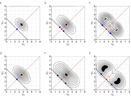
The set of equations given by Eq. (23) and Eq. (21) con-stitute three equations for the three unknowns{η1, η2, λ}. We proceed to solve these numerically, and plot the resulting solutions in Fig. 1. The free parameters in the problem are {µ, η?
1, η?2, α,σ, η¯ obs}. Figure 1 displays
re-sults such that for each of two values of ¯σ (each value corresponds to a row of the plot), the parameter control-ling the non-Gaussianity, namely µ, is varied over three possible values from 0 to 0.1 to 1 (from left to right). Each value corresponds to a column of the plot. We choose ηobs = 5 (which is, recall, approximately the ex-perimentally observed value),η?
1 = 3.6 =η2?(so that the distribution has weight near the experimentally observed value), andα=−0.5 (for illustrative purposes).
We see that in the Gaussian case (µ = 0, Fig. 1a, 1d), there is a single maximum (blue circle) which oc-curs atη1 =ηobs/2 = η2 in accord with the general re-sult derived earlier [Eq. (14)]. When we break Gaussian-ity we overturn this result. For smaller deviations from Gaussianity (µ = 0.1, Fig. 1b, 1e), the maxima on the constraint surface correspond to (two symmetric cases in which) one component slightly dominates over the other (with a roughly 3:2 split in Fig. 1b and a roughly 3.4:1.6 split in Fig. 1e). There is also a single (local) minimum on the constraint surface between these maxima, whose probability is close to theirs. This result is amplified in the case where the non-Gaussianity is stronger (µ= 1, Fig. 1c, 1f). The maxima on the constraint surface have
a probability that is significantly greater than the single (local) minimum (by a factor of&2), and the dominance of one component is also greater than in theµ= 0.1 case, with a roughly 3.5:1.5 split in Fig. 1c, and a roughly 3.7:1.3 split in Fig. 1f.
Atypicality therefore predicts either the existence of two equally contributing components [corresponding to the local minima (red squares) in Fig. 1c, 1f] or indeed just a single dominant component (that is more domi-nant than the prediction under typicality, that is, as one moves along the constraint surface towards either axis in Fig. 1c, 1f, say1).
Thus we have exhibited a scenario in the top-down approach where: atypicality corresponds to equal con-tributions, and typicality to unequal contributions (i.e., one dominant species), to the total dark matter density. Non-Gaussianities can change the nature of the predic-tion.
IV. ANTHROPIC CONDITIONALIZATION
Anthropic conditionalization represents an intermedi-ate point between bottom-up and top-down approaches in that some multiverse domains are indeed excised in the computation of probabilities but the restriction is not as stringent as in the case of top-down conditionalization.
From a calculational point of view, as discussed in Aguirre and Tegmark [10], one can implement an-thropic conditionalization by adopting a weighting fac-tor W that multiplies the raw probability distribution P(~η|T) and expresses the probability of finding domains in which we might exist, as a function of the relevant parameter we are investigating. In Aguirre and Tegmark [10], and in what follows, the assumption is made that W ≡W(η) is a function of the total dark matter density η≡PN
i=1ηi, and we will look into the effects of assum-ing an η-dependent Gaussian fall-off for this weighting factor. That is, we will assume, following [10] that
W(η)∝exp
− 1 2η2
0 η2
, (24)
1Note that one would need to worry about boundary conditions
η1
η
2
a
0 1 2 3 4 5 6 7 8
0 1 2 3 4 5 6 7 8
η
1η
2
b
0 1 2 3 4 5 6 7 8
0 1 2 3 4 5 6 7 8
η1
η
2
c
0 1 2 3 4 5 6 7 8
0 1 2 3 4 5 6 7 8
η1
η
2
d
0 1 2 3 4 5 6 7 8
0 1 2 3 4 5 6 7 8
η
1η
2
e
0 1 2 3 4 5 6 7 8
0 1 2 3 4 5 6 7 8
η1
η
2
f
0 1 2 3 4 5 6 7 8
0 1 2 3 4 5 6 7 8
FIG. 1. Contour plots of the distributionQ(η1, η2|T) [see Eq. (20)]. In each panel, the black line denotes the constraint surface, and the red line denotes the line of equal density. Along the constraint surface, blue circles correspond to (global) maxima and red squares to (local) minima. Note that in (b,c,e,f), pairs of maxima have the same probability in each panel. Parameters have been set as follows: ηobs = 5, η1? = 3.6 = η2?, and α = −0.5. (a–c) ¯σ = ηobs/6 with µ = 0,0.1,and 1 respectively. (d–f) ¯σ = ηobs/5 with µ = 0,0.1,and 1 respectively. The Gaussian cases (a,d) exhibit a single maximum corresponding to equal contributions to the total dark matter density from the two components (as discussed in section III A). The equality of contribution is overturned in a significant way forµ= 1, that is (c,f), where in each case, the maxima correspond to unequal contributions and the local minimum corresponds to equal contributions.
where we also assume that we have a way of calculating the standard deviation η0.2 The optimization problem that implements the assumption of typicality now de-mands that we maximize the total probability
distribu-2 Note that for the sake of calculational simplicity, we extend
the domain of validity of the Gaussian fall-off for the anthropic weighting factorW(η), beyond that explored in [10], where this domain corresponded toη > η0. This raises a subtlety regarding
the value(s) ofη that can appropriately be considered to max-imizeW(η). This is a debate that lies outside the scope of the problem considered in this paper, but would need to be addressed in a less stylized setting.
tionPtot(~η|T, W), which takes this anthropic weighting factor into account, where
Ptot(~η|T, W)∝P(~η|T)W(η). (25)
We will investigate the result of doing this for the corre-lated Gaussian case discussed in Sec. III, beginning first with the case where we do not restrict the covariance matrix. In addition, in contrast to our discussion so far, we will focus less on the equality of contribution of dif-ferent components to the total dark matter density; and more on a new feature that arises exclusively in the an-thropic approach: that of the determination of precisely
dark matter density.
A. The optimization routine
We assume again, that there are N possible species of dark matter and that we need to find the value of ~η
such thatPtot(~η|T, W) is maximized, where, substitut-ing Eq. (3) and Eq. (24) into Eq. (25), we have
Ptot(~η|T, W)∝exp
−1 2
N
X
i,j=1
(ηi−ηi?)(C
−1)
ij(ηj−ηj?)
exp
− 1 2η2
0 η2
. (26)
For eachk, setting∂lnPtot(~η|T, W)/∂ηk = 0 gives
N
X
i=1
(ηi−ηi?)(C
−1)
ik=−
1 η2
0
η. (27)
Multiplying through by Ckj, summing over k and
rear-ranging, we find
ηj=η?j−
1 η2
0 η
N
X
k=1
Ckj. (28)
As in section III A, choosing theη?
j’s and/or the sums of
the columns of the covariance matrix appropriately, one can find contributions to the total dark matter density such that all species do not contribute equally.
However, under the assumption that ηj? = ¯η for all j [i.e., Eq. (10)], and that the covariance matrix is given by Eq. (11) say, we recover the case of equal contributions discussed above. In particular, we obtain, for eachj,
ηj = ¯η−
1 η2
0
η[1 + (N−1)α] ¯σ2, (29)
where the right-hand side does not depend on j. The solution to these equations is just ηj = γ, say, so that
η≡PN
i=1ηi=N γ. Thus we find
ηj=γ=
¯ η η2
0 η2
0 +N¯σ2[1 + (N−1)α]
. (30)
In addition, the optimal total densityηoptis given by
ηopt=N γ =N
¯ ηη2
0 η2
0 +Nσ¯2[1 + (N−1)α]
. (31)
There is another way one can derive this last result [Eq. (31)], which is helpful in understanding the nature of the optimization being carried out, and so we outline the results of this alternate derivation here. Namely, when P(~η|T) is Gaussian with mean vector (η1?, η?2, . . . , ηN?) and covariance matrixC [as in Eq. (3)], then the prob-ability distribution over the sum PN
i=1ηi ≡ η, denoted
byR(η), is also Gaussian with mean PN
i=1η
?
i and
vari-ance PN
i,j=1Cij (see for example [30, chapter II, Sec.
13]). Under the simplifying assumptions introduced ear-lier, namely, if we set η?
i = ¯η for all i, and C → C˜ as
in Eq. (11), we have: PN
i=1η
?
i = Nη¯ and
PN
i,j=1Cij = Nσ¯2[1 + (N−1)α]. Thus
R(η)∝exp
− 1
2Nσ¯2[1 + (N−1)α](η−Nη)¯ 2
. (32)
The resulting probability distribution over the sum of the densitiesη, denoted byPtot(η|T, W), can be shown to be:
Ptot(η|T, W)∝R(η)W(η)
= exp
− 1
2Nσ¯2[1 + (N−1)α](η−Nη)¯ 2
exp
− 1 2η2
0 η2
= exp
− 1
2Σ2(η−Φ) 2
, (33)
where
Σ2= η 2
0Nσ¯2[1 + (N−1)α] η2
0 +Nσ¯2[1 + (N−1)α]
, (34)
Φ =N ηη¯
2 0 η2
0 +Nσ¯2[1 + (N−1)α]
. (35)
displayed in Eq. (31).
B. Prediction and fine tuning
How then, in light of the above discussion, do we pro-pose to extract a prediction fromPtot(η|T, W) while al-lowing for variations in assumptions regarding typicality? We know that the probability distributionPtot(η|T, W) is Gaussian [see Eqs. (33), (34), and (35)], and so it has a single maximum; moving sufficiently far away from this maximum takes us into regions of atypicality. Hence, in-troducing a factor F >0 that measures deviations from the maximum, we propose that the framework specified by the theoryT, together with the anthropic conditional-ization factorW(η), and the typicality assumption char-acterized byF, is
predictive if 1
Fηopt=ηobs, (36)
where F = 1 corresponds to the assumption of ‘maxi-mum’ typicality, and deviations from F = 1 correspond to some degree of atypicality.
In addition, following Aguirre and Tegmark [10], we do not want this prediction to be too finely tuned, in the sense that increasing the value of the prediction (i.e., F1ηopt) should not take us too far into the tail of the anthropic conditionalization factor W(η) [given by Eq. (24)]. In this way, we will assume that the value of the prediction for the total observed dark matter density is
not finely tuned if 1
Fηopt≤2η0, (37) namely, within two standard deviations, 2η0, of the mean of the Gaussian conditionalization factorW(η). The pre-cise tolerance here is less important than the general con-clusions we will develop below.
We will show (as indeed mentioned by Aguirre and Tegmark [10]) that the criteria expressed in Eqs. (36) and (37) can be used to predict the total number of equally contributing components to the total dark mat-ter density, and it is within the context of this type of prediction that we will analyze the effects of atypicality. To gain intuition about how these two criteria operate, we begin by analyzing the case of independent species of dark matter.
C. Independent species and typicality assumptions
In the case of independent species of dark matter, namely, when α = 0, a quick calculation reveals that the prediction that F1ηopt=ηobs [Eq. (36)], in combina-tion with Eq. (31), can be translated into a prediccombina-tion
forN, with
N = F ηobsη 2 0 η2
0η¯−F ηobsσ¯2
. (38)
The demand that the original prediction is not finely tuned, namely, that F1ηopt ≤ 2η0 [Eq. (37)], bounds N such that
N ≤ 2F η 2 0
η0η¯−2Fσ¯2, (39)
forη0η >¯ 2Fσ¯2; otherwise no such upper bound exists. Equations (38) and (39) imply that if 0< F <1, both the value ofN that is predictive and the upper bound on N such that the prediction is not finely tuned, decrease relative to the case of typicality (i.e., relative toF = 1). WhenF >1, these values increase relative to the case of typicality. In this way, atypicality can change the nature of the prediction.
D. Correlated species and typicality assumptions
For nonzero α, again using Eq. (31), we find that the framework we are examining is predictive, i.e., satisfies Eq. (36), when
αηobs¯σ2N2+
(1−α)ηobsσ¯2− 1 Fηη¯
2 0
N+ηobsη02= 0,
(40) and this prediction is not finely tuned, i.e., satisfies Eq. (37), when
−2α¯σ2N2+
1
Fηη0¯ −2¯σ
2(1−α)
N−2η02≤0. (41)
We note that now, depending on the balance of the pa-rameters in the problem, it is possible that under the inclusion of nonzero correlations, there exist two distinct solutions to the prediction for the total number of species that contribute equally to the total dark matter density. We focus first on this effect in more detail, before study-ing the effects of atypicality on the resultstudy-ing predictions. In particular, we will be interested in two different ques-tions: (1) under the assumption of typicality, how does a nonzero α change predictions for N (relative to the α= 0 case, and assuming these predictions are not finely tuned), and (2) for a fixed nonzero α, how does atypi-cality change the prediction forN (again assuming these predictions are not finely tuned)?
1. The effect of correlations,α6= 0, onN, under typicality
original probability distribution P(~η|T) has significant probability near the observed value; more precisely, we will assume
¯
η≡ηobs, (42)
and (ii) that the variance of the conditionalization factor W(η) is related in a simple way to the variances of the dark matter components,
η02=Xσ¯2, (43)
for some positiveXwhose range will be specified shortly. Under these assumptions then, the prediction for the number of uncorrelated species, as derived from Eq. (38), and which we will now refer to asN0, is
N0= X
X−1. (44)
In order thatN0is a physically realizable prediction (and so that we do not, at this stage, discount the framework that gave rise to this prediction), we choose X > 1, so thatN0>1.
Similarly, these assumptions imply that Eq. (40) re-duces to
αNα2+ (1−α−X)Nα+X = 0, (45)
where we now denoteN byNα; the solution of which is
Nα=
X+α−1±p
(1−α−X)2−4αX
2α . (46)
Let us note a couple of cases of interest here. Firstly, if (1−α−X)2= 4αX, then there is just a single solution Nα= (X+α−1)/2α. Settingα= 0.25 for example, gives
X = 2.25 and soNα= 3 whereasN0≈2 (one can show
that both of these solutions are not necessarily finely tuned). In the case that (1−α−X)2>4αX,N
0will ex-hibit just a single solution, whereasNα may exhibit two
(physical) solutions. Figure 2 displays some illustrative examples of what these solutions look like. There we ex-hibit solutionsN0(red circles) andNα(blue squares) for
α= 0.25, under the assumption thatX = 2.35,2.5,or 2.7 (corresponding to Fig. 2a, 2b, or 2c respectively). We see that in Figs. 2a and 2b, the introduction of correla-tions leads to two distinct solucorrela-tions for Nα, the greater
of which is significantly different from N0. In the case of Fig. 2c, the smaller of the two solutions for Nα is
discounted as unphysical (as only those solutions in the correlated case make sense whereNα≥2).
2. How does atypicality change the prediction whenα6= 0?
The second question we are interested in is the nature of the change in the prediction as a result of atypical-ity in the correlated Gaussian case. To investigate this in a simple setting, we again invoke the assumptions of
section IV D 1 as expressed in Eqs. (42) and (43). The equation expressing predictivity, Eq. (40), reduces to
αNα2+ (1−α− 1
FX)Nα+X = 0, (47)
and the bound on Nα such that the prediction is not
finely tuned, namely Eq. (41), reduces to
−2α¯σNα2+
1
Fηobs √
X−2¯σ(1−α)
Nα−2X¯σ≤0.
(48) For illustrative values of the parameters, the effects of these equations on the prediction of the total number of species of dark matter contributing equally to the total dark matter density are explored in Fig. 3. We see there that the prediction under the assumption of atypicality [as determined by the appropriatex-axis-intercept(s) of the black parabola in each panel; recall that only those solutions whereNα≥2 are considered physical] changes
significantly from the prediction under the assumption of typicality [corresponding to the appropriate x-axis-intercept(s) of the gray parabola in each panel].
V. DIFFERENT FRAMEWORKS, SAME PREDICTION
So let us recapitulate what we have found thus far, in order to better understand the nature of the overlaps that exist between different frameworks as regards their predictions for the total number of species of dark matter that we should expect to observe.
In the case of bottom-up conditionalization (Sec. II), where we assumed the underlying probability distribu-tionP(~η|T) was unimodal and could, in principle, take nonzero values within some N-dimensional cube in pa-rameter space, the expected number of dominant dark matter components, under the assumption of typicality, was shown to be 1. In the terminology of Sec. II,hji ∼1 forM N. However, atypicality can change this pre-diction to a range of other possibilities, including equal contributions from allN components.
atypi-N
a
1 2 3 4 5
−1 0 1
N
b
1 2 3 4 5 6
−1 0 1
N
c
1 2 3 4 5 6 7
−1 0 1
FIG. 2. Change in the prediction for N in the presence of correlations under the assumption of typicality. (a,b,c) exhibit solutions for the choicesX = 2.35,2.5,and 2.7 respectively. The red circles correspond toN0, the prediction for independent species of dark matter [see Eq. (44)—each of these solutions is not finely tuned under the choice of parameters described herein]. The parabolas correspond to the left-hand side of Eq. (45), whosex-axis-intercepts are the predictions forNα, shown in blue squares, whereα= 0.25 in each case [a prediction ofNα<2, as for the smaller of the two predictions in (c), is discounted as ‘unphysical’]. The gray segments overlapping thex-axes correspond to the range of solutions that are not finely tuned for the correlated case (namely, the region of thex-axis where the constraint given by Eq. (41) is satisfied—recall thatF = 1 under the assumption of typicality, and we have set ¯η=ηobs, andη2
0 =Xσ¯2). We have setηobs= 5 in accord with the experimentally observed value, and for the sake of illustration, we have set ¯σ2= 2.8. We note that in (a,b), there exist two, distinct, physically acceptable predictions forNα, the greater of which is also significantly different from the case where there are no correlations.
cality corresponds to equal contributions, or indeed to a single species dominating to a greater degree than in the case of typicality (as in Fig. 1c and 1f).
Finally, for the anthropic case (Sec. IV), we explored the assumption of atypicality in a different way to the first two approaches: namely, by tracking its impact on the total numberN of equally contributing components (indeed, in Sec. IV,N could vary, unlike in the bottom-up and top-down cases where it was fixed by assump-tion at the outset). Now, under typicality, correlaassump-tions in the underlying probability distribution can change the prediction for N relative to the independent case (see Fig. 2), and it is possible for two physically acceptable predictions to exist, which again, can change quantita-tively under the assumption of atypicality (as in Fig. 3). It is evident from the above discussion that the types of prediction discussed here do not cleanly discriminate be-tween frameworks consisting of theory, conditionalization scheme and typicality assumption. For example, consider first the prediction that dark matter consists of a single dominant component. This could be derived from each conditionalization scheme studied above in (at least) the following ways:
— bottom-up: for anN-dimensional unimodal distri-bution under typicality (Sec. II);
— top-down: for uncorrelated or correlated N -dimensional Gaussians under atypicality [Eq. (19), and items (i) and (ii) at the end of Sec. III B], or the 2-dimensional non-Gaussian distribution of Eq. (20) under typicality (Fig. 1c and 1f);
— anthropic: for uncorrelated Gaussians assuming typicality, Eqs. (42), (43), and X 1 [so that Eq. (44) impliesN0∼1].
The prediction of multiple species of dark matter does not fare any better in terms of its ability to discrim-inate between frameworks. Consider the prediction of two equally dominant species of dark matter. This could also be derived from each conditionalization scheme in (at least) the following ways:
— bottom-up: for an N-dimensional unimodal distri-bution under an appropriate assumption of atypi-cality (as discussed at the end of Sec. II);
— top-down: for correlated 2-dimensional Gaussians under typicality (see Fig. 1a and 1d), or the 2-dimensional non-Gaussian distribution of Eq. (20) under atypicality (see Fig. 1c and 1f);
— anthropic: for correlated Gaussians under typical-ity (as in the smaller of the two distinct predictions of Fig. 2a and 2b) or from the smaller of two dis-tinct predictions under atypicality (as in Fig. 3b and 3d).
a
N
α1 2 3 4 5 6 7 8
−2 −1 0 1
b
N
α1 2 3 4 5 6 7 8
−2 −1 0 1
c
N
α1 2 3 4 5 6 7 8 9
−2 −1 0 1
d
N
α1 2 3 4 5 6 7 8 9
−2 −1 0 1
FIG. 3. The effects of atypicality on the prediction ofNα, where α= 0.25. (a)X = 2.5,F = 0.875; (b)X = 2.5,F = 1.05; (c)X = 2.7,F = 0.875; (d)X = 2.7,F = 1.05. In each case, we have also setηobs= 5 and ¯σ2 = 2.8. For each panel, the intersection of the gray parabola with thex-axis corresponds to the prediction under typicality, whereas the intersection of the black parabola with thex-axis, marked by blue squares, corresponds to the prediction under the assumption of atypicality (recall that we accept only those solutions for which Nα ≥2). The gray segment overlapping thex-axis corresponds to the range of solutions for the atypical scenario that are not finely tuned. We see in each case that predictions for Nα can shift significantly.
VI. DISCUSSION
For theories that describe a multiverse, the confirma-tion of these theories must—short of direct experimental evidence—rest on tests such as those explored in this paper. Any such theory will probably describe an over-whelming number of domains that look nothing like ours, in which case theory alone will not be enough to extract meaningful predictions. Indeed, conditionalization will be needed, in which we restrict attention to domains in such a way as to sharpen the comparison between what the theory predicts and what we observe.
Any of the conditionalization schemes outlined by Aguirre and Tegmark [10] and studied herein, or
in-deed more sophisticated versions of these, are plausible candidates; but there is an inherent arbitrariness in the choice. And as explored in this paper, the situation is further complicated by assumptions regarding typicality.
(such as the outcomes of future experiments) can take different values in these domains, the appropriate test of the conjunction will be a comparison of what we observe with what the conjunction predicts for our observations (a first-person prediction, in the terminology of Srednicki and Hartle [14]). We cannot know, of course, which of these domains we are in and so to extract an appropri-ate prediction, we need to make an assumption about our typicality with respect to these domains. Under such circumstances, the assumption that we are typical is cer-tainly not guaranteed a priori; and so it makes sense to then allow for a variety of assumptions regarding typ-icality in order to identify the most predictive frame-work [14, 26].
In this paper we have taken seriously the conclusions of the last paragraph, and have applied them to the com-parison of the total number of observed species of dark matter with predictions generated from some theory of the multiverse. A central feature has been that what such a comparison tests is an entire framework, namely, a conjunction of theory, conditionalization scheme, and typicality assumption. Hence if the prediction of such a conjunction does not match our observations, we must disfavor the entire conjunction; and thus we have license to change any of its conjuncts, and to then reassess the predictive power of the resulting framework. What we find under this scenario, as argued in this paper, is a com-plex set of interconnected relationships between frame-works and predictions. Indeed, as drawn out in Sec. V,
the same prediction can arise from distinctly different frameworks.
It would be interesting to see how widespread these ‘overlaps’ are for more realistic cosmological scenarios. If they are also robust to the choice of the physical observ-ables we aim to predict the values of, and we believe that truly distinct frameworks indeed give rise to the same prediction, then we are forced to conclude that the pre-diction cannot confirm any single framework taken on its own. Of course, one has recourse to more intricate confirmation schemes, such as those invoked in Bayesian analyses—which would introduce priors over frameworks to help in their demarcation (see [14, 23] for example). But in the context where we focus solely on likelihoods (as we have implicitly done in this paper), robust over-laps between frameworks present an acute challenge for the utility of such tests of the multiverse.
ACKNOWLEDGMENTS
I am very grateful to Jeremy Butterfield for discus-sions and comments on an earlier version of this paper, and to Jim Hartle for posing a question over email at an early stage, which helped to guide my thoughts along the general lines expressed in this paper. I am supported by the Wittgenstein Studentship in Philosophy at Trinity College, Cambridge.
[1] Paul Joseph Steinhardt, “Natural inflation,” inThe Very Early Universe, Proceedings of the Nuffield Workshop, Cambridge, 21 June to 9 July, 1982, edited by G.W. Gibbons, S.W. Hawking, and S.T.C. Siklos (Cambridge University Press, Cambridge, 1983).
[2] Alexander Vilenkin, “Birth of inflationary universes,” Phys. Rev. D27, 2848–2855 (1983).
[3] A. D. Linde, “Chaotic inflation,” Phys. Lett.129B, 177– 181 (1983).
[4] A. D. Linde, “Eternal chaotic inflation,” Mod. Phys. Lett. A01, 81–85 (1986).
[5] A. D. Linde, “Eternally existing self-reproducing chaotic inflationary universe,” Phys. Lett. B 175, 395–400 (1986).
[6] Raphael Bousso and Joseph Polchinski, “Quantization of four-form fluxes and dynamical neutralization of the cosmological constant,” J. High Energy Phys. 06 (2000) 006.
[7] Shamit Kachru, Renata Kallosh, Andrei Linde, and Sandip P. Trivedi, “de Sitter vacua in string theory,” Phys. Rev. D68, 046005 (2003).
[8] Ben Freivogel, Matthew Kleban, Mar´ıa Rodr´ıguez Mart´ınez, and Leonard Susskind, “Ob-servational consequences of a landscape,” J. High Energy Phys. 03 (2006) 039.
[9] Leonard Susskind, “The anthropic landscape of string theory,” in Universe or Multiverse?, edited by B. Carr (Cambridge University Press, Cambridge, 2007).
[10] Anthony Aguirre and Max Tegmark, “Multiple universes, cosmic coincidences, and other dark matters,” J. Cosmol. Astropart. Phys. 01 (2005) 003.
[11] Anthony Aguirre, “Making predictions in a multiverse: conundrums, dangers, coincidences,” inUniverse or Mul-tiverse?, edited by B. Carr (Cambridge University Press, Cambridge, 2007).
[12] Steven Weinstein, “Anthropic reasoning and typicality in multiverse cosmology and string theory,” Classical Quan-tum Gravity23, 4231–4236 (2006).
[13] J. Garriga and A. Vilenkin, “Prediction and explanation in the multiverse,” Phys. Rev. D77, 043526 (2008). [14] Mark Srednicki and James Hartle, “Science in a very
large universe,” Phys. Rev. D81, 123524 (2010). [15] James Hartle and Thomas Hertog, “Anthropic bounds
on Λ from the no-boundary quantum state,” Phys. Rev. D88, 123516 (2013).
[16] James Hartle and Thomas Hertog, “The observer strikes back,” arXiv:1503.07205.
[17] Brandon Carter, “Large number coincidences and the an-thropic principle in cosmology,” inConfrontation of Cos-mological Theories with Observational Data, IAU Sympo-sium No. 63, edited by M. S. Longair (D. Reidel Publish-ing Company, Dordrecht & Boston, 1974) pp. 291–298. [18] James B. Hartle, “Anthropic reasoning and quantum
principle for our future prospects,” Nature363, 315–319 (1993).
[20] Alexander Vilenkin, “Predictions from quantum cosmol-ogy,” Phys. Rev. Lett.74, 846–849 (1995).
[21] Don N. Page, “Sensible quantum mechanics: Are prob-abilities only in the mind?” Int. J. Mod. Phys. D 05, 583–596 (1996).
[22] Nick Bostrom,Anthropic Bias: Observation Selection Ef-fects in Science and Philosophy (Routledge, New York, 2002).
[23] James B. Hartle and Mark Srednicki, “Are we typical?” Phys. Rev. D75, 123523 (2007).
[24] Lee Smolin, “Scientific alternatives to the anthropic prin-ciple,” in Universe or Multiverse?, edited by B. Carr (Cambridge University Press, Cambridge, 2007). [25] Feraz Azhar, “Prediction and typicality in multiverse
cos-mology,” Classical Quantum Gravity31, 035005 (2014). [26] Feraz Azhar, “Testing typicality in multiverse
cosmol-ogy,” Phys. Rev. D91, 103534 (2015).
[27] Gianfranco Bertone, Dan Hooper, and Joseph Silk, “Par-ticle dark matter: evidence, candidates and constraints,” Phys. Rep.405, 279–390 (2005).
[28] Max Tegmark, Anthony Aguirre, Martin J. Rees, and Frank Wilczek, “Dimensionless constants, cosmology, and other dark matters,” Phys. Rev. D 73, 023505 (2006).
[29] P. A. R. Ade et al. (Planck Collaboration), “Planck 2015 results. XIII. Cosmological parameters,” arXiv:1502.01589.