www.geosci-model-dev.net/8/533/2015/ doi:10.5194/gmd-8-533-2015
© Author(s) 2015. CC Attribution 3.0 License.
Firedrake-Fluids v0.1: numerical modelling of shallow water flows
using an automated solution framework
C. T. Jacobs and M. D. Piggott
Department of Earth Science and Engineering, Imperial College London, London SW7 2AZ, UK Correspondence to: C. T. Jacobs ([email protected])
Received: 14 August 2014 – Published in Geosci. Model Dev. Discuss.: 27 August 2014 Revised: 22 January 2015 – Accepted: 9 February 2015 – Published: 9 March 2015
Abstract. This model description paper introduces a new fi-nite element model for the simulation of non-linear shallow water flows, called Firedrake-Fluids. Unlike traditional mod-els that are written by hand in static, low-level programming languages such as Fortran or C, Firedrake-Fluids uses the Firedrake framework to automatically generate the model’s code from a high-level abstract language called Unified Form Language (UFL). By coupling to the PyOP2 parallel unstruc-tured mesh framework, Firedrake can then target the code towards a desired hardware architecture to enable the effi-cient parallel execution of the model over an arbitrary com-putational mesh. The description of the model includes the governing equations, the methods employed to discretise and solve the governing equations, and an outline of the auto-mated solution process. The verification and validation of the model, performed using a set of well-defined test cases, is also presented along with a road map for future developments and the solution of more complex fluid dynamical systems.
1 Introduction
Traditional approaches to numerical model development in-volve the production of hand-written, low-level (e.g. C or Fortran) code for the specific set of equations that need to be solved. This task alone can be highly error-prone, often resulting in sub-optimal code, and can make the efficiency, readability, and longevity of the code base difficult to main-tain (Rognes et al., 2013; Farrell et al., 2013; Mortensen et al., 2011; Maddison and Farrell, 2014). Moreover, paral-lelisation of the code is usually accomplished by introduc-ing explicit calls to parallel programmintroduc-ing libraries such as OpenMP or CUDA (Compute Unified Device Architecture).
By doing so, computational scientists are frequently faced with the additional task of having to re-write their model’s code as new parallel hardware architectures and platforms emerge. At the current rate that new hardware is introduced, this development workflow is unsustainable and places an infeasible requirement on the developer to be not only a subject/domain specialist adept in computational methods but also well versed in software engineering and paralleli-sation principles. A change to the traditional programming paradigm is clearly necessary if numerical model develop-ment is to continue in a sustainable manner.
mod-els to be written with just a few lines of high-level intuitive code (although the potential of writing fewer, more intuitive lines of model code is not unique to automated code genera-tion approaches, as demonstrated by the interfaces of other modelling frameworks such as OpenFOAM (OpenFOAM, 2014), deal.II (Bangerth et al., 2007), Dune (Dedner et al., 2010) and FreeFem++ (Hecht, 2012)). Several other applica-tion areas using automated soluapplica-tion techniques have demon-strated similar benefits (see, e.g., the works by Farrell et al., 2013; Funke and Farrell, 2013; Logg et al., 2012).
The Firedrake project aims to further extend the abstrac-tions offered by automated solution approaches, by creating a separation of concerns between the automated low-level discretisation of the model equations and its execution on the underlying computational mesh (Rathgeber et al., 2015), whilst still keeping the same high-level problem solving in-terface for end users. This provides the potential for easier portability of the generated code across different hardware platforms (e.g. multi- and many-core CPUs and GPUs), as well as the efficient handling of computations over a given mesh topology (e.g. taking advantage of the semi-structured nature of a three-dimensional layered mesh extruded in the vertical, as often employed in ocean/atmospheric applica-tions). This is achieved by interfacing with the PyOP2 par-allel unstructured mesh computation framework, which tar-gets the automatically generated code towards specific high-performance computing platforms (Rathgeber et al., 2012; Markall et al., 2013; Luporini et al., 2015). In addition, the enhanced abstraction-based approach employed by Firedrake can also help future-proof models from hardware changes and removes a great deal of effort required by computational scientists to maintain the code base.
In light of the issues surrounding the use of static, hand-coded numerical models and the benefits that the Fire-drake framework can bring, a new numerical model called Firedrake-Fluids has been developed for computational fluid dynamics (CFD)-related applications. The long-term goal of the project is to facilitate a re-engineering of Fluidity (Pig-gott et al., 2008), another CFD package (also developed at Imperial College London) comprising hand-written Fortran code whose efficiency, readability, and longevity has become challenging to maintain as the package has grown over many years. In contrast to Fluidity, Firedrake-Fluids has been writ-ten in the high-level Unified Form Language (UFL) and uses Firedrake to automate the solution process. Currently it is capable of solving the non-linear shallow water equations which are widely used in the ocean modelling community for applications such as tidal turbine dynamics (Divett et al., 2013; Kramer et al., 2014; Martin-Short et al., 2015), array optimisation (Funke et al., 2014), tsunami modelling (Hill et al., 2014), flow dynamics over submerged islands (Lloyd and Stansby, 1997), and dam breaching and flooding (Capart and Young, 1998). In addition to the core model, Firedrake-Fluids offers upwind stabilisation methods, a variety of di-agnostic fields, and the Smagorinsky large-eddy simulation
H
h
Figure 1. Diagram showing the mean free surface heightH (also
known as the depth or the distance to the seabed, shaded grey) and the free surface perturbationh, within the shallow water model.
(LES) model (Smagorinsky, 1963) for the parameterisation of turbulence.
Section 2 details the set of equations that are solved and the assumptions under which they are valid. Section 3 describes the numerical methods that are used to discretise and solve the governing equations, followed by an overview of the automated solution techniques employed by the Firedrake framework. Section 4 presents results from a suite of test cases used to verify the correctness of the numerical model’s implementation, and show how well it describes the physics. A discussion regarding the future developments and direc-tion of Firedrake-Fluids is presented in Sect. 5, along with some concluding remarks in Sect. 6.
2 Model equations
The model described in this paper solves the non-linear, non-rotational shallow water equations. These are a set of depth-averaged equations which model the dynamics of a free surface and an associated depth-averaged velocity field (Zhou, 2004). This velocity field is denoted byu=u(x, y, t )
(where x andy are the spatial coordinates, andt is time). For modelling purposes, the free surface is split up into a mean componentH=H (x, y) and a perturbation compo-nenth=h(x, y, t )as illustrated in Fig. 1. Note thathis gen-erally assumed to be much smaller thanH.
2.1 Momentum equation
The momentum equation is solved in non-conservative form such that
∂u
∂t +u· ∇u= −g∇h+ ∇ ·T−CD
||u||2u
(H+h), (1)
where t is time, g is the acceleration due to gravity (set to 9.8 ms−2 throughout this paper), and CD is a
non-dimensional drag coefficient. The Euclidean norm ||u||2= √
u·u is used here, and throughout the rest of this paper. The stress tensorTis given by
T=ν ∇u+ ∇uT−2
3ν (∇ ·u)I, (2)
whereν is the kinematic viscosity, which is assumed to be isotropic here, andIis the identity tensor1.
2.2 Continuity equation The continuity equation is given by
∂h
∂t + ∇ ·((H+h)u)=0. (3)
2.3 Initial and boundary conditions
In order to advance the equations forward in time, initial con-ditions for the prognostic fieldshandu
h(x, y, t=0)=h0,u(x, y, t=0)=u0, (4) must be specified.
Throughout the simulation, values of the free surface per-turbation fieldhmay be enforced (in the strong sense) at the boundary using a Dirichlet boundary condition
h=hD on0, (5)
where 0⊂is the portion of the boundary on which the boundary condition (hD in this case) is applied. Note that this boundary condition can vary both in time and in space.
In addition to the standard Dirichlet boundary condition for the velocity field
u=uD on0, (6)
1The interior penalty method (Arnold, 1982) is applied to the
stress term when using discontinuous basis functions for the ve-locity field (see Sect. 3.2), since the gradient of veve-locity has to be treated carefully at the boundaries between discontinuous elements. Although it is possible to extend the UFL implementation to the full stress tensor, the current implementation of the method restricts the form toT=ν∇ufor simplicity. In the near-future when tensor function spaces are supported in the Firedrake library, the Bassi– Rebay method (Bassi and Rebay, 1997) will be implemented in-stead and will consider the full form of the stress tensor.
whereuD is the value of the velocity to be enforced at the boundary, there are two other conditions that may be applied. The no-normal flow condition enforces
u·n=0 on0, (7)
wherenis the unit normal vector.
The Flather (1976) boundary condition enforces
u−u∗=
r
g
H(h−h∗) on0, (8)
whereu∗andh∗are the expected velocity and free surface
perturbation exterior to the domain, respectively. Any dif-ference between the expected and simulated free surface is allowed to propagate out of the domain, thereby minimis-ing spurious reflections from the boundary. Note that both of these boundary conditions can only be applied in the weak sense; the velocity value must be applied in the surface inte-gral term, which only appears if the divergence term in the continuity equation is integrated by parts. An option for do-ing this is available in the simulation configuration file, dis-cussed later in Sect. 3.4.
2.4 Turbulence modelling
The core shallow water model on its own has no way of cap-turing the effects of turbulence, unless the underlying mesh is of a suitably fine resolution to perform a direct numerical simulation at all turbulence length scales. This is often pro-hibitively expensive, and so turbulence parameterisation is required. The Smagorinsky LES model represents one possi-ble way of doing this. It parameterises the turbulence via an eddy viscosity (Smagorinsky, 1963; Deardorff, 1970)
ν0=(Cs1e)2|S|, (9)
whereCs is the Smagorinsky coefficient, and1e is an
es-timate of the local mesh size which is defined here as the square root of the area of each element (in the 2-D case).|S|
is the modulus of the strain rate tensor defined by
S=
1
2 ∇u+ ∇u
T
,|S| =
s 2X
i
X
j
SijSij, (10)
whereSij is the (i,j)th component ofS. The eddy viscosity
ν0, which models the dissipating effects of small-scale tur-bulent eddies on the resolved flow, is added to the physical viscosityνin the stress term of the momentum equation.
3 Methods
3.1 Automated code generation
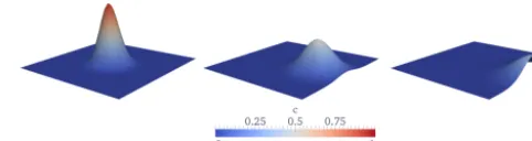
Figure 2. Sample Python code which uses the high-level Unified
Form Language (UFL) to solve the advection–diffusion equation with the finite element method. The solution fieldchas a Gaussian profile att=0, which is then advected with a prescribed velocity fieldu= [0.1,0]T.
with associated boundary and initial conditions) to be discre-tised (both temporally and spatially) and expressed in a near-mathematical language called UFL, an embedded language that uses Python as its host (Alnæs et al., 2014). An example of a model defined in UFL which solves a two-dimensional advection–diffusion problem is given in Fig. 2 (with associ-ated results in Fig. 3), and highlights how the implementa-tion can be accomplished with just a few lines of intuitive statements. This one file containing approximately 50 lines of UFL is automatically compiled into over 600, much more complicated, lines of low-level C code which are executed over the entire mesh by PyOP2 to perform the assembly of the finite element system.
The UFL code is compiled at runtime, using a modified version of the FEniCS form compiler (FFC)2 (Kirby and
2The original version of FFC, which is part of the FEniCS
project, compiles the UFL into low-level C++ code called UFC
Figure 3. Visualisation of the solution fieldcatt=0, 2.5, and 5 s from the advection–diffusion problem defined in Fig. 2. The initial Gaussian profile is advected from left to right, out of the domain, and slowly diffuses over time. The field has been warped in thez direction.
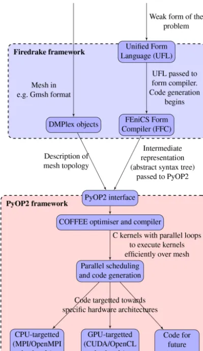
Logg, 2006; Luporini et al., 2015), into an intermediate rep-resentation as an abstract syntax tree (AST) before being passed into the PyOP2 library, as shown in Fig. 4. Further-more, optimal numbering of the solution nodes in the domain is important to avoid cache misses and ensure efficient com-putation; therefore, the topology of any mesh that is provided by the user (e.g. from the Gmsh mesh generator (Geuzaine and Remacle, 2009)) is described using a PETSc (Portable, Extensible Toolkit for Scientific Computation) DMPlex ob-ject which is also passed to PyOP2 along with the AST. PyOP2 then performs additional optimisations on the AST using the COFFEE (COmpiler For FinitE Element local as-sembly) compiler (Luporini et al., 2015) which outputs the model’s optimised low-level C code. Finally, PyOP2 calls a back-end compiler (e.g. GNU gcc or the Intel C compiler for CPUs) to compile the generated code on demand at runtime (known as just-in-time compilation), and then executes it ef-ficiently over the entire domain. As previously mentioned, in addition to targeting the code towards multi-core CPUs, PyOP2 can also target the generated code towards a specific parallel platform using, for example, the PyOpenCL and Py-CUDA compilers for GPUs. Note that, however, as a result of current implementation restrictions (e.g. the solution of non-linear problems is not yet possible with PyOP2 on GPUs) the work presented in this paper only considers the compilation of code using the GNU gcc compiler on CPUs.
3.2 Spatial and temporal discretisation
The spatial discretisation of the model equations is per-formed using the Galerkin finite element method. The first step of the method involves deriving the variational/weak form of the model equations by multiplying them by a so-called test functionw∈H1()3, whereH1()3is the first (Kirby and Logg, 2006; Logg and Wells, 2010), whereas the mod-ified version in Firedrake first compiles the UFL into an abstract syntax tree (AST) for further manipulation and optimisation by the PyOP2 framework (Luporini et al., 2015). The modified ver-sion of FFC is available from the MAPDES Bitbucket reposi-tory: https://bitbucket.org/mapdes/ffc. Revision6c0d70d in the
Figure 4. Overview of the key components of the Firedrake and
PyOP2 frameworks (Rathgeber, 2014).
Hilbertian Sobolev space (Elman et al., 2005), and integrat-ing them over the whole domain; this yields, in the case of the momentum equation, Eq. (1),
Z
w·∂u
∂t dV+
Z
w·(u· ∇u)dV =
−
Z
gw· ∇hdV−
Z
∇w·TdV
−
Z
CDw· ||u||2u
(H+h) dV .
Note that the stress term has been integrated by parts and it is assumed that the normal stress gradient at all boundaries is zero. In this weak form, a solutionu∈H1()3is sought for allw∈H1()3.
The test function and the solutionu(also known as the trial function) are then replaced by discrete representations, given by a linear combination of basis functions{φi}
Nu_nodes i=1 which
may be continuous or discontinuous across the cells/elements
of the mesh:
w=
Nu_nodes
X
i=1
φiwi, (11)
u=
Nu_nodes
X
i=1
φiui, (12)
whereNu_nodesis the number of velocity solution nodes in
the mesh,wi are arbitrary, and the coefficientsui are sought
using a numerical solution method. The free surface pertur-bation fieldh, which needs to be solved for in addition to the velocity field, is also represented by a (possibly different) set of basis functions{ψi}Nh_nodesi=1 :
h=
Nh_nodes
X
i=1
ψihi, (13)
whereNh_nodesis the number of free surface solution nodes,
andhi are the coefficients to be found.
The discrete system of sizeNu_nodes×Nu_nodesfor the
mo-mentum equation then becomes M∂u
∂t +A(u)u= −Ch−Ku−D(u, h)u, (14)
where M, A, K, C and D are the mass, advection, stress, gra-dient, and drag discretisation matrices, respectively. The no-tations A(u)and D(u, h)are used to highlight the non-linear dependence of the matrices on the velocity and free surface fields. A similar process is performed for the continuity equa-tion, Eq. (3), resulting in a full block-coupled system.
The temporal discretisation, performed using the implicit backward Euler method, yields
Mu
n+1−un
1t +A(u
n+1)un+1=
−Chn+1−Kun+1−D(un+1, hn+1)un+1,
where the superscriptnrepresents the current time level and
n+1 represents the next time level. The backward Euler method gives first-order accuracy in time. Newton iteration is employed to deal with the non-linearity introduced via the advection and drag terms, although this does not need to be implemented explicitly by the model developer; instead, it can be performed using a PETSc Scalable Nonlinear Equa-tions Solvers (SNES) object. Other temporal discretisation approaches such as the Crank–Nicolson method can be read-ily implemented in UFL, but are not currently available in Firedrake-Fluids.
for velocity and piecewise-linear basis functions for the free surface) element pairs will be considered. Unless otherwise stated, the P2–P1 element pair will be used in preference to P0–P1, in order to obtain higher-order solutions. However, users are free to choose the order and continuity of the ba-sis functions through the simulation configuration file (dis-cussed in Sect. 3.4). Currently, Firedrake-Fluids only allows Lagrange polynomial basis functions to be used, although other basis function families are available through FIAT (e.g. Raviart–Thomas).
In Sect. 2, it was mentioned that the form of the stress ten-sor is currently restricted in the case of using discontinuous basis functions. In the future, once tensor function spaces be-come available in the Firedrake framework, the Bassi–Rebay method (Bassi and Rebay, 1997) will be implemented instead and will consider the full form of the stress tensor. In addi-tion, some more complicated numerical techniques cannot be formulated in the UFL language, such as slope limiters. How-ever, it is possible to implement them in lower-level code in the form of a PyOP2 C kernel which interacts directly with the nodal data to accomplish this.
3.3 Solution methods
Firedrake assembles the full block-coupled form of the dis-crete system of linear equations, and attempts to solve it us-ing the PETSc library (Balay et al., 2014). PETSc contains a variety of linear solvers and preconditioners, and has proven itself in facilitating geoscientific model development (Katz et al., 2007). It is possible to use, for example, the generalised minimal residual method (GMRES) or conjugate gradient it-erative method, and preconditioners such as Jacobi and SOR (successive over-relaxation). For the simulations presented in this paper, the GMRES linear solver (Saad and Schultz, 1986) is chosen and used in conjunction with the fieldsplit preconditioner (Brown et al., 2012) which is especially suited to block-coupled systems such as the one considered here.
The block-coupled system takes the general form
A B
C D
u h
=
fu
fh
(15) for matrix blocks A, B, C and D, and right-hand sides fuand
fh.
The matrix on the left-hand side can be factorised using LDU (lower-diagonal-upper) block factorisation to give (El-man et al., 2008)
I 0
CA−1 I
A 0 0 S
I A−1B
0 I
, (16)
where S=D−CA−1B is the Schur complement. The inverse of the factorised system is given by
P =
I −A−1B
0 I
A−1 0 0 S−1
I 0
−CA−1 I
. (17)
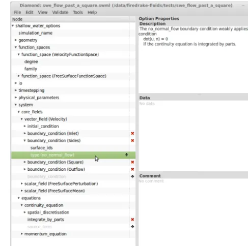
Figure 5. The Diamond (Ham et al., 2009) graphical user interface
for editing Firedrake-Fluids simulation configuration files.
It is the goal of the fieldsplit preconditioner to find approx-imations to the actions of S−1and A−1 which will in turn give an approximation to the action of P which can be used to precondition the block-coupled system. PETSc features a wide configuration space for its fieldsplit preconditioner, per-mitting the use of different iterative (or direct) solvers and preconditioners for the sub-problems S−1 and A−1. Unless stated otherwise, incomplete LU (ILU) factorisation will be used as an approximate solver for S−1and A−1in all simula-tions presented here (except when running in parallel, where block Jacobi is applied globally and the individual blocks are solved sequentially using ILU (Balay et al., 2014)). The con-vergence criterion for all iterative solvers is a relative error of 10−7.
3.4 Set-up and execution
All UFL model code is stored in themodelsdirectory of Firedrake-Fluids. Execution of, for example, the shallow wa-ter model is performed by calling the Python inwa-terprewa-ter and providing the path to the simulation configuration file; an ex-ample for the test case involving flow past a square cylinder (discussed in Sect. 4) would be
python models/shallow_water.py tests/swe_flow_past_a_square/
swe_flow_past_a_square.swml.
Simulation settings are first read in using the libspud
library (Ham et al., 2009). This is followed by the execu-tion of the UFL statements which define the model. Note that the weak form of the shallow water equations is defined in UFL only once, before entering the time-stepping loop. Upon entering the time-stepping loop for the first time, the form is compiled and the low-level assembly code is gener-ated. For subsequent time steps, caching is used such that no re-compilation of the UFL is necessary. Solution fields are currently written to files in Visualization Toolkit format for visualisation.
Note that the UFL code for the LES model described in Sect. 2.4 is defined in a separate class within the Firedrake-Fluids package (in the fileles.py) for modularity, and to facilitate its use in future numerical models that may re-quire turbulence parameterisation. In the case of the shal-low water model implemented in shallow_water.py, the UFL for the left-hand side and right-hand side of the eddy viscosity equation, Eq. (9), is first imported, and a separate solver computes the eddy viscosity field at the start of each time step, using the velocity from the previous time step. The viscosity used in the stress term is then updated, but doing so does not require the re-compilation of the UFL. Similarly, at the end of each time step inshallow_water.py, di-agnostic fields, such as the divergence of a vector field, the Courant number, or the grid Peclet number field, can be com-puted. The routines used to compute these diagnostic fields are contained indiagnostics.py.
4 Verification and validation
The following subsections describe some of the key verifi-cation and validation test cases included in Firedrake-Fluids. These tests are executed using the Buildbot automated test-ing framework whenever a change is made to the software (Farrell et al., 2011) to ensure that any bugs introduced dur-ing the development of Firedrake-Fluids (or through the de-velopment of Firedrake itself and other dependencies such as PETSc) are detected and promptly resolved by the develop-ers.
4.1 Convergence analysis
Since no general analytical solution to the shallow wa-ter equations exists, the method of manufactured solutions
Table 1. Parameters used in the MMS test cases.
Parameter Description Value CD Drag coefficient 0.0025
ν Kinematic viscosity 0.6 m2s−1 H Mean free surface height 20 m
(MMS) (Roache, 2002) was used to perform a convergence analysis and verify the correctness of the model implementa-tion. The first step of MMS involves inventing or manufactur-ing a function and modifymanufactur-ing the original equation such that this manufactured function is the analytical solution of the modified equation. Substituting this function into the shallow water equations will generate a non-zero source term which can then be placed on the right-hand side, such that the man-ufactured/invented solution is now the analytical solution to this modified set of equations.
A two-dimensional domain with dimensions 0≤x≤1 m and 0≤y≤1 m was used for the MMS simulations. Simu-lations were run with three different structured meshes with characteristic element lengths 1x=0.2, 0.1 and 0.05 m, comprising 36, 121, and 441 vertices, respectively. The time steps were set to 1t=0.01, 0.005, and 0.0025 s, respec-tively, to enforce a near-constant bound on the Courant num-ber. A zero initial condition was used for both the velocity and free surface fields, and Dirichlet boundary conditions which agreed with the analytical/manufactured solutions for the velocity and free surface were enforced along all walls of the domain. All simulations were run until the steady-state conditions||un+1−un||2≤10−6and||hn+1−hn||2≤10−6 were attained.
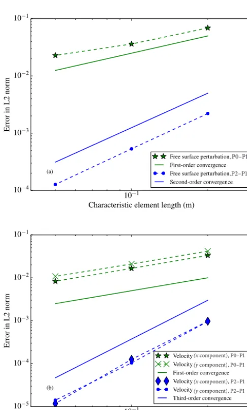
Both the P2–P1 and P0–P1 element pairs were considered. The manufactured solutions wereh=sin(x)sin(y)andu= [cos(x)sin(y),sin(x2)+cos(y)]T. The physical parameters, given in Table 1, were chosen arbitrarily and used across all the simulations.
10−1
Characteristic element length (m)
10−4
10−3
10−2
10−1
Erro
rin
L2
no
rm
Free surface perturbation, P0-P1 First-order convergence Free surface perturbation, P2-P1 Second-order convergence (a)
10−1
Characteristic element length (m)
10−5
10−4
10−3
10−2
10−1
Erro
rin
L2
no
rm
Velocity (x-component), P0-P1 Velocity (y-component), P0-P1 First-order convergence Velocity (x-component), P2-P1 Velocity (y-component), P2-P1 Third-order convergence (b)
1
P0–P1
P2–P1
(x component), P0–P1 (y component), P0–P1
(x component), P2–P1 (y component), P2–P1
Figure 6. The orders of convergence for (a) the free surface field
and (b) the velocity field, in the P2–P1 and P0–P1 MMS test cases.
In the case of P0–P1, both the velocity and free surface perturbation fields exhibited only first-order spatial conver-gence. Whilst second-order spatial convergence may have been expected for the free surface field because of the use of a P1 function space, the reduced order of convergence was likely the result of the coupling between the fields and the use of a first-order upwind scheme for the advection term at dis-continuous element boundaries. The low-order scheme may have introduced additional, dominating error that polluted both solution fields via the coupled system, thereby keeping the overall spatial convergence at no higher than first-order.
All simulations were run in serial on a dual-core Intel Core i7-3537U processor with a clock speed of 2 GHz and at least 2 GB of available RAM. In the P2–P1 case, the runtimes were 3.8, 6.9, and 31.7 s, for the meshes with1x=0.2, 0.1, and 0.05 m, respectively. Note that these simulations were run with a warm cache such that the high-level UFL has already
been compiled down to low-level C code; from a cold cache (i.e. including the code compilation time), the runtimes were 9.4, 12.5, and 37.7 s. In both the P2–P1 and P0–P1 cases, the simulations typically required 2–3 non-linear Newton itera-tions per time step, and the number of GMRES solver iter-ations taken per non-linear iteration varied between 12 and 17. However, in the P0–P1 case, the warm cache runtimes were significantly larger as a result of more time steps being required to reach steady state: 41.4, 85.8, and 177.8 s. 4.2 Dam failure
Dam failure (also known as dam break) problems are com-monly used to test the performance of shallow water mod-els. The presence of a discontinuity in the initial condition makes them particularly difficult to accurately solve. Both one-dimensional and two-dimensional results are presented.
The one-dimensional case considers a channel 0 ≤x≤
2000 m. A dam wall is located atx=1000 m which holds back the water contained in the upstream reservoir. The water in the reservoir has a total depth of 10 m, whilst downstream the total water depth is set to 5 m. The water is initially at rest. Att=0 the dam is instantaneously removed, thereby simulating its failure, allowing water to rush into the down-stream section. Typical shock characteristics for the velocity and free surface perturbation fields were observed and com-pared well with the semi-analytical solutions of the corre-sponding one-dimensional Riemann problem shown in Fig. 7 att=60 s. Note that the simulation used an element length of1x=5 m and a time step of 0.25 s, as per the simulations of Liang et al. (2008) which consider the same scenario. The kinematic viscosity was set to 1 m2s−1, and the drag coeffi-cient was set to zero.
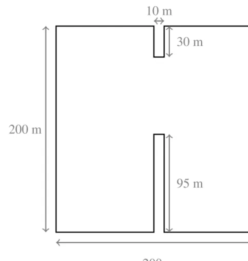
The two-dimensional case considers a square domain with dimensions 0≤x≤200 m and 0≤y≤200 m. A 10 m thick dam is placed in the centre of the domain as shown in Fig. 8. In this scenario, only a partial failure of the dam is simu-lated; water rushes into the downstream area through a 75 m long breach in the dam wall. As before, the water is initially at rest. The upstream reservoir contains water with a total height of 10 m, whilst the downstream section contains water with a total height of 5 m. No-normal flow boundary condi-tions are applied along all walls (including those of the dam). Once again, the time step (1t=0.2 s) and the characteristic element length (1x=5 m) were the same as those chosen by Liang et al. (2008). The kinematic viscosity was set to 1 m2s−1, and the drag coefficient was set to zero.
re-0 500 1000 1500 2000
x(m) 0
1 2 3 4 5
Free
surf
ace
perturbation
(m)
Numerical (Firedrake-Fluids) Analytical
(a)
0 500 1000 1500 2000
x(m) 0.0
0.5 1.0 1.5 2.0 2.5 3.0
V
elocity
(ms
−
1)
Numerical (Firedrake-Fluids) Analytical
(b)
Figure 7. Numerical solutions of the 1-D dam failure problem. The
semi-analytical solutions, found by solving a set of equations de-fined in the book by Trangenstein (2009), are also plotted.
sults closely agree with those from the numerical simulations by Liang et al. (2008) and Mingham and Causon (1998). 4.2.1 Solver performance
The performance of the iterative solver in combination with the fieldsplit preconditioner was investigated on a much larger system. The mesh was refined such that the charac-teristic element length was set to1x=0.25 m, resulting in 817 488 vertices. The time step1twas also lowered to 0.01 s to maintain the same upper bound on the Courant number. The strong scaling of the iterative solver (GMRES, with the fieldsplit preconditioner) and the assembly of the system is shown in Fig. 10. All of these performance simulations were performed on ARCHER (a Cray XC30 supercomputer), comprising 12-core Intel Ivy Bridge processors running with
200 m
200 m
10 m
30 m
95 m
Figure 8. Dimensions of the domain for the 2-D dam failure
prob-lem. The dam (with a 75 m wide breach) is situated in the centre.
a clock speed of 2.7 GHz, with 32 GB of RAM available to each one.
The GMRES iterative method was also used in conjunc-tion with the SOR precondiconjunc-tioner when computing the acconjunc-tion of the matrices A−1and S−1. This resulted in fewer outer it-erations (typically 2 or 3) when solving the block-coupled system as a whole as a result of a better preconditioned sys-tem. On the other hand, ILU decomposition provided a rela-tively less accurate approximation to A−1and S−1(resulting in typically 10–30 outer iterations) but was faster than the GMRES with SOR runs, as shown in Fig. 10, despite the extra outer iterations. It is for this reason that ILU factori-sation was used as the preconditioner of the sub-problems A−1 and S−1 throughout this paper. Note that smaller sys-tems with1x=0.5 m and 1 m were also investigated; it was found that the number of solver iterations was near constant as the size of the system changed, regardless of the set-up of the fieldsplit preconditioner.
4.3 Tidal flow over a regular bed
The test case described by Bermudez and Vazquez (1994) considers tidal flow in a one-dimensional domain of length
L=14 000 m. The mean water height (and hence the topog-raphy of the bed) is defined by
H (x)=50.5−40x
L −10 sin
π
4x
L −
1 2
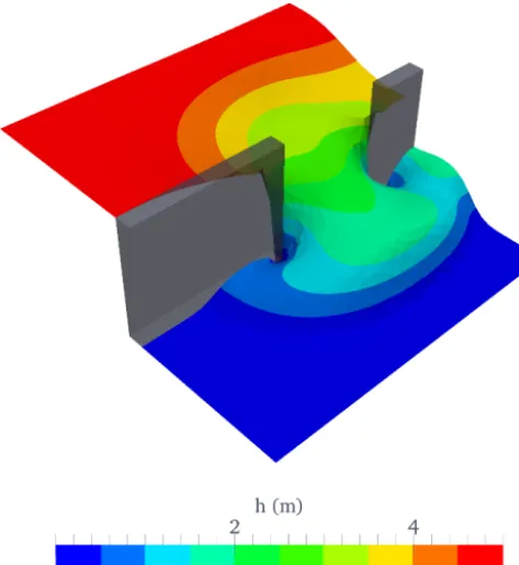
Figure 9. Free-surface perturbationhat timet=7.2 s, from the 2-D dam failure simulation. The field has been warped in thezdirection to emphasise the collapse of the water column.
for the free surface and velocity:
h(0, t )=4−4 sin
π
4t 86 400+
1 2
, (19)
to simulate an incoming sinusoidally varying tidal wave, and
u(L, t )=0, (20)
at the outflow boundary.
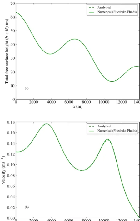
This simulation was performed with a mesh element length of1x=14 m. The time step1t was set to 2.5 s and the simulation finished at t=9117.5 s (the same time con-sidered by Zhou, 2004). The kinematic viscosity was set to 1 m2s−1, and the drag coefficient was set to zero. The results in Fig. 11 illustrate how the velocity of the flow increases in deeper regions of the body of water as expected. The nu-merical results also display good accuracy with the analytical solutions given by Bermudez and Vazquez (1994), thereby further validating the numerical model. The total runtime of the simulation was 26 min when run in serial on a dual-core Intel Core i7-3537U processor with a clock speed of 2 GHz and at least 2 GB of available RAM.
4.4 Tidal flow over an irregular bed
A second version of the tidal flow test case considered pre-viously is one that involves an irregular bed topology, with sharp peaks and troughs which can be a challenge to repre-sent accurately. This test case is described by Zhou (2004).
100 101 102 103
Number of MPI processes 100
101
102
103
104
To
tal
time
tak
en
to
co
mp
lete
10
time step
s
(s)
GMRES with SOR (Solver) GMRES with SOR (Assembly) Incomplete LU (Solver) Incomplete LU (Assembly) Ideal speed-up
Figure 10. Strong scaling of the 2-D dam break simulation, with
1x=0.25 m. The total runtime spent in the assembly and solver over 10 time steps is shown. The internal Firedrake/PyOP2 and PETSc timers were used to obtain the timing data. As expected, the time spent in assembly does not vary significantly between runs since it is independent of the difference in solver set-ups.
The test case considers a one-dimensional domain of length L=1500 m. The irregular topography of the bed
B(x)is defined in Table 2, and the mean water height is given by H (x)=20−B(x). The initial conditions h(x,0)= −4 andu(x,0)=0 are applied along with the following Dirich-let boundary conditions for the free surface and velocity:
h(0, t )= −4 sin
π
4t 86 400+
1 2
, (21)
u(L, t )=0. (22) The element length1x=7.5 m and the time step 1t=
0.3 s, as per the set-up of Zhou (2004). The simulation was performed untilt=10 800 s. All remaining components of the set-up were the same as the regular bed test case de-scribed in Sect. 4.3.
Figure 12 once again demonstrates a good match between the numerical results and the analytical solution, and demon-strates the robustness of the numerical model in accurately representing more rapidly varying areas of the solution. The total runtime of the simulation was 56.7 min when run in serial on a dual-core Intel Core i7-3537U processor with a clock speed of 2 GHz and at least 2 GB of available RAM. 4.5 Flow past a square cylinder
Figure 11. Numerical solutions from the tidal flow simulation over
a regular bed, att=9117.5 s. The analytical solutions are given by Bermudez and Vazquez (1994) and almost completely overlap the numerical solutions. Note that the free surface plot (a) includes the mean free surface height, such that theyaxis representsh+H.
turbulent flow past a square cylinder. The set-up used in the experiments by Lyn and Rodi (1994) and Lyn et al. (1995) (and the numerical simulations by Rodi et al., 1997) was con-sidered.
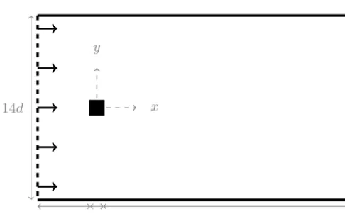
The dimensions of the domain are given in terms of the width/length of the squared=0.04 m in Fig. 13. An unstruc-tured mesh with a characteristic element length1x=d/15, generated with Gmsh (Geuzaine and Remacle, 2009), was used; this value of 1x is comparable to the minimum el-ement lengths used in the numerical simulations presented in the paper by Rodi et al. (1997). The free surface mean height was set toH=4d(the depth of the experimental flow tank). The physical kinematic viscosity of the fluid was set to 10−6m2s−1, which corresponded to a Reynolds number of 21 400 when usingd as the length scale. The Smagorinsky coefficientCsin the Smagorinsky LES model (Smagorinsky,
1963) was set to 0.164, within the typical range ofCsvalues
(Deardorff, 1971).
Table 2. Bed heights along the seabed from Zhou (2004).
x Bed height (m) B(x)(m)
0 0
50 0
100 2.5
150 5
250 5
300 3
350 5
400 5
425 7.5
435 8
450 9
475 9
500 9.1
505 9
530 9
550 6
565 5.5 575 5.5
600 5
650 4
700 3
750 3
800 2.3
820 2
900 1.2 950 0.4
1000 0
1500 0
Initially the velocity and free surface perturbation fields were set to zero. At the inlet, a constant velocity boundary condition of 0.535 ms−1was enforced; the inflow was lami-nar and no turbulent eddies were seeded along the boundary. No-normal flow boundary conditions were applied along the side walls, whilst no-slip boundary conditions were applied along all walls of the square. At the outflow, a Flather bound-ary condition (Flather, 1976) (specifying an external velocity equal to that at the inlet, and a free surface perturbation of zero) was used to allow flow out of the domain whilst min-imising reflections. A time step of1t=5×10⁻⁴s was cho-sen, and the simulation was performed untilt=15 s.
The simulation was performed on ARCHER (a Cray XC30 supercomputer) using two 12-core Intel Ivy Bridge proces-sors running with a clock speed of 2.7 GHz, with 32 GB of RAM available to each one. The total run time was 7.7 h.
simula-Figure 12. Numerical solutions from the tidal flow simulation with
an irregular bed topography. The analytical solutions (Zhou, 2004; Bermudez and Vazquez, 1994) agree very well with the numerical solutions from Firedrake-Fluids.
x y
14d
4.5d d 19.5d
Figure 13. The dimensions of the two-dimensional domain
contain-ing a square cylinder (filled black) of length/widthd. The incoming flow is from the left boundary, as denoted by the black arrows.
tion time. The vortex street is clearly visible in Fig. 14 which shows thexcomponent of the velocity field att=10 s.
The stream-wise velocity along the centreline, time-averaged over a period of 15 s from the start of the simula-tion, was compared with the experimental data presented by Lyn et al. (1995) and Rodi et al. (1997); the results in Fig. 15 show a good match with the experimental data behind the square cylinder in the recirculating region where turbulent vortex shedding occurs, thereby illustrating the benefits of using the Smagorinsky LES model to accurately capture the turbulent flow characteristics. However, the wake recovery region was poorly represented; the unfortunate lack of accu-racy in this region has also been observed in other numerical models (Rodi et al., 1997), and additional parameterisations and the full three-dimensionality of the problem may need to be considered to properly represent the wake.
5 Road map
The long-term aim is to extend Firedrake-Fluids into a suite of numerical models which encompass a much wider range of flow types, as well as additional equation sets (e.g. the full Navier–Stokes equations) and constitutive equations (e.g. for describing Darcy’s law in porous media). Essentially, Firedrake-Fluids seeks to facilitate a complete re-engineering of the Fluidity CFD code, whilst maintaining the mature modelling functionality that Fluidity offers. In addition to the potential for portability of the low-level code across dif-ferent back ends, such as the Intel C compiler and CUDA, it is hoped that Firedrake will also enable the portability of the code’s performance. This has yet to be demonstrated on large-scale problems, and will therefore be one of the main focusses of this work in the future.
One of the first application areas that Firedrake-Fluids will consider, using the shallow water model described in this pa-per, is flow around tidal turbines. This will contribute to an on-going effort towards understanding the potential of re-newable energy systems. The multi-scale nature of the ap-plication will necessitate the use of high-performance com-puting, and Firedrake’s ability to target code towards more modern hardware architectures such as GPU clusters will be utilised. Regarding the application area itself, the integration of adjoint optimisation models is of particular related inter-est. For example, recent progress in the optimisation of the layout of a tidal turbine farm using the FEniCS automated solution framework has proven to be a successful technique for maximising the theoretical amount of generated power (Funke et al., 2014). The DOLFIN-adjoint library (Farrell et al., 2013) was used for this purpose. Although FEniCS and Firedrake both expect UFL statements as input, not all of the UFL interfaces are compatible with each other at present; a similar adjoint library for Firedrake (Firedrake-adjoint) is therefore under development by the authors of DOLFIN-adjoint, and its use in the shallow water model is one of the shorter-term goals of the Firedrake-Fluids project. The issue of compatibility is being addressed by the developers of Fire-drake.
dis-Figure 14. Visualisation of thexcomponent of the velocity field, from the simulation of flow past a square att=10 s.
Figure 15. Time-averaged stream-wise velocity along the centreline
from the simulation of flow past a square. Note that the velocity has been normalised by the inlet velocityU=0.535 ms−1.
continuous Galerkin method will also be implemented. It is expected that a large proportion of this work will need to be undertaken within the Firedrake and PyOP2 frameworks, in addition to Firedrake-Fluids, in order to correctly describe the mesh topology (including that of the dual mesh in the case of control volume methods).
6 Conclusions
This model description paper has introduced a new open-source finite element model, Firedrake-Fluids, for the sim-ulation of shallow water flows. The model is written in the high-level, near-mathematical UFL and uses the Firedrake framework (coupled with the PyOP2 library) to automate the
solution process. Furthermore, the Firedrake library provides the potential for porting the code across to different hardware back ends, although this has not been demonstrated here and will be a consideration of future work. The automated solu-tion approach allows the focus to be on the equasolu-tions that are solved and the numerical results, and removes the require-ment for model developers to be experts in parallel program-ming and software engineering. Furthermore, the high-level specification of the problem facilitates better maintainability of the Firedrake-Fluids code base; in comparison with the shallow water model in the Fluidity CFD code, which fea-tures static hand-written Fortran, the Firedrake-Fluids source code is considerably shorter and more intuitive. This is a result of the near-mathematical notation used, and the fact that code generation and assembly are handled by the exter-nal Firedrake and PyOP2 libraries. Firedrake-Fluids uses ap-proximately 400 lines (excluding comments and blank lines), compared to many thousands to perform the same task in Fluidity. Note that the 400 lines include code to obtain user settings, initial conditions, etc., from the simulation configu-ration file, and to make the model as generic as possible; if the model were to be written for a specific set-up, the number of lines could potentially be further minimised to just a few dozen. It should be noted that this benefit is not unique to the Firedrake-Fluids model nor to UFL in general, since it is also possible to write models with a relatively small amount of code with other packages such as OpenFOAM (OpenFOAM, 2014), deal.II (Bangerth et al., 2007), Dune (Dedner et al., 2010), and FreeFem++ (Hecht, 2012).
At runtime, the high-level model specification defined in Firedrake-Fluids is converted by Firedrake (and the PyOP2 framework) into optimised, low-level C code. This is then compiled with a back-end compiler appropriate for the tar-get architecture; however, this work has only considered the GNU gcc compiler for CPUs, since it is not yet possible to as-semble and run the non-linear problems detailed in this paper on GPUs. As new high-performance architectures are intro-duced in the future, only the PyOP2 layer which deals with code targeting needs to be modified; model developers are not burdened with the task of specialising the model code it-self, which is presently a common problem even in modern finite element models.
Code availability
Firedrake-Fluids is an open-source software package that has been released under the GNU General Public License (Version 3). The code base is hosted by GitHub in a pub-lic repository and can be obtained at the following URL: https://github.com/firedrakeproject/firedrake-fluids. The par-ticular version of Firedrake-Fluids considered in this paper (version 0.1) is available from the releases page.
Acknowledgements. The authors would like to acknowledge funding from Imperial College London and an ARCHER eCSE grant (eCSE03-7). The authors also acknowledge the use of the Imperial College High Performance Computing Service, and the UK National Supercomputing Service (ARCHER). Thoughtful reviews from Marie Rognes and Andreas Dedner were gratefully received.
Edited by: H. Weller
References
Alnæs, M. S., Logg, A., Ølgaard, K. B., Rognes, M. E., and Wells, G. N.: Unified Form Language: A domain-specific language for weak formulations of partial differential equations, ACM Trans. Math. Softw., 40, 9, doi:10.1145/2566630, 2014.
Arnold, D. N.: An Interior Penalty Finite Element Method with Discontinuous Elements, SIAM J. Num. Analysis, 19, 742–760, doi:10.1137/0719052, 1982.
Balay, S., Abhyankar, S., Adams, M., Brown, J., Brune, P., Buschel-man, K., Eijkhout, V., Gropp, W., Kaushik, D., Knepley, M., Curfman McInnes, L., Rupp, K., Smith, B., and Zhang, H.: PETSc Users Manual, Tech. Rep. Revision 3.5, Argonne Na-tional Laboratory, 2014.
Bangerth, W., Hartmann, R., and Kanschat, G.: deal.II–A general-purpose object-oriented finite element library, ACM Trans. Math. Softw., 33, 24, doi:10.1145/1268776.1268779, 2007.
Bassi, F. and Rebay, S.: A High-Order Accurate Discontinuous Fi-nite Element Method for the Numerical Solution of the Com-pressible Navier-Stokes Equations, J. Comput. Phys., 131, 267– 279, doi:10.1006/jcph.1996.5572, 1997.
Bermudez, A. and Vazquez, M. E.: Upwind methods for hyperbolic conservation laws with source terms, Comput. Fluids, 23, 1049– 1071, doi:10.1016/0045-7930(94)90004-3, 1994.
Brown, J., Knepley, M. G., May, D. A., McInnes, L. C., and Smith, B. F.: Composable Linear Solvers for Multiphysics, in: Proceeedings of the 11th International Symposium on Parallel and Distributed Computing (ISPDC 2012), 55–62, doi:10.1109/ISPDC.2012.16, 2012.
Capart, H. and Young, D. L.: Formation of a jump by the dam-break wave over a granular bed, J. Fluid Mech., 372, 165–187, doi:10.1017/S0022112098002250, 1998.
Deardorff, J.: A numerical study of three-dimensional turbulent channel flow at large Reynolds numbers, J. Fluid Mech., 41, 453– 480, doi:10.1017/S0022112070000691, 1970.
Deardorff, J. W.: On the magnitude of the subgrid scale eddy coefficient, J. Comput. Phys., 7, 120–133, doi:10.1016/0021-9991(71)90053-2, 1971.
Dedner, A., Klöfkorn, R., Nolte, M., and Ohlberger, M.: A generic interface for parallel and adaptive discretization schemes: Ab-straction principles and the DUNE-FEM module, Computing, 90, 165–196, doi:10.1007/s00607-010-0110-3, 2010.
Divett, T., Vennell, R., and Stevens, C.: Optimization of multiple turbine arrays in a channel with tidally reversing flow by numer-ical modelling with adaptive mesh, Philos. Trans. Roy. Soc. A, 371, 1471–2962, doi:10.1098/rsta.2012.0251, 2013.
Elman, H., Howle, V. E., Shadid, J., Shuttleworth, R., and Tu-minaro, R.: A taxonomy and comparison of parallel block multi-level preconditioners for the incompressible Navier-Stokes equations, J. Computat. Phys., 227, 1790–1808, doi:10.1098/rsta.2012.0251, 2008.
Elman, H. C., Silvester, D. J., and Wathen, A. J.: Finite Elements and Fast Iterative Solvers: with applications in incompressible fluid dynamics, Oxford University Press, 2005.
Farrell, P. E., Piggott, M. D., Gorman, G. J., Ham, D. A., Wil-son, C. R., and Bond, T. M.: Automated continuous verifica-tion for numerical simulaverifica-tion, Geosci. Model Dev., 4, 435–449, doi:10.5194/gmd-4-435-2011, 2011.
Farrell, P. E., Ham, D. A., Funke, S. W., and Rognes, M. E.: Au-tomated derivation of the adjoint of high-level transient finite el-ement programs, SIAM J. Scientific Comput., 35, C369–C393, doi:10.1137/120873558, 2013.
Flather, R. A.: A tidal model of the northwest European continental shelf, Memoires de la Société Royale des Sciences de Liège, 10, 141–164, 1976.
Funke, S. W. and Farrell, P. E.:A framework for automated PDE-constrained optimisation, arXiv:1302.3894, submitted, 2013. Funke, S. W., Farrell, P. E., and Piggott, M. D.: Tidal turbine array
optimisation using the adjoint approach, Renewable Energy, 63, 658–673, doi:10.1016/j.renene.2013.09.031, 2014.
Geuzaine, C. and Remacle, J.-F.: Gmsh: A 3-D finite element mesh generator with built-in pre- and post-processing facilities, Int. J. Num. Methods Eng., 79, 1309–1331, doi:10.1002/nme.2579, 2009.
Ham, D. A., Farrell, P. E., Gorman, G. J., Maddison, J. R., Wilson, C. R., Kramer, S. C., Shipton, J., Collins, G. S., Cotter, C. J., and Piggott, M. D.: Spud 1.0: generalising and automating the user interfaces of scientific computer models, Geosci. Model Dev., 2, 33–42, doi:10.5194/gmd-2-33-2009, 2009.
Hecht, F.: New development in FreeFem++, J. Num. Math., 20, 251–265, doi:10.1515/jnum-2012-0013, 2012.
Hill, J., Collins, G. S., Avdis, A., Kramer, S. C., and Pig-gott, M. D.: How does multiscale modelling and inclu-sion of realistic palaeobathymetry affect numerical simulation of the Storegga Slide tsunami?, Ocean Model., 83, 11–25, doi:10.1016/j.ocemod.2014.08.007, 2014.
Katz, R. F., Knepley, M. G., Smith, B., Spiegelman, M., and Coon, E. T.: Numerical simulation of geodynamic processes with the Portable Extensible Toolkit for Scientific Computation, Phys. Earth Planet. Int., 163, 52–68, doi:10.1016/j.pepi.2007.04.016, 2007.
Kirby, R. C. and Logg, A.: A compiler for varia-tional forms, ACM Trans. Math. Softw., 32, 417–444, doi:10.1145/1163641.1163644, 2006.
Kramer, S. C., Piggott, M. D., Hill, J., Kregting, L., Pritchard, D., and Elsaesser, B.: The modelling of tidal turbine farms using multi-scale, unstructured mesh models, in: Proceedings of the 2nd International Conference on Environmental Interac-tions of Marine Renewable Energy Technologies, (EIMR2014), Stornoway, Scotland, 2014.
Liang, S.-J., Tang, J.-H., and Wu, M.-S.: Solution of shallow-water equations using least-squares finite-element method, Acta Me-chanica Sinica, 24, 523–532, doi:10.1007/s10409-008-0151-4, 2008.
Lloyd, P. M. and Stansby, P. K.: Shallow-Water Flow around Model Conical Islands of Small Side Slope. II: Submerged, J. Hydraul. Eng., 123, 1068–1077, doi:10.1061/(ASCE)0733-9429(1997)123:12(1068), 1997.
Logg, A. and Wells, G. N.: DOLFIN: Automated finite element computing, ACM Trans. Math. Softw., 37, 20, doi:10.1145/1731022.1731030, 2010.
Logg, A., Mardal, K.-A., Wells, G. N., Alnæs, M. S., Clark, S. R., Davidson, D. B., Vilela de Abreu, R., Degirmenci, C., Haga, J. B., Hake, J., Hoffman, J., Jansson, J., Jansson, N., Johnson, C., Kirby, R. C., Knepley, M. G., Langtangen, H. P., Lezar, E., Linge, S., Logg, A., Lopes, N. D., Løvgren, A. E., Mardal, K.-A., Mortensen, M., Narayanan, H., Nazarov, M., Nikbakht, M., Pereira, P. J. S., Ring, J., Rognes, M. E., Schroll, H. J., Scott, L. R., Selim, K., Støle-Hentschel, S., Terrel, A. R., Trabucho, L., Valen-Sendstad, K., Vynnytska, L., Wells, G. N., Wilbers, I. M., and Ølgaard, K. B.: Automated Solution of Differential Equa-tions by the Finite Element Method, Springer, doi:10.1007/978-3-642-23099-8, 2012.
Luporini, F., Varbanescu, A. L., Rathgeber, F., Bercea, G.-T., Ra-manujam, J., Ham, D. A., and Kelly, P. H. J.: Cross-Loop Optimization of Arithmetic Intensity for Finite Element Lo-cal Assembly, ACM Trans. Archi. Code Optimization, 11, 57, doi:10.1145/2687415, 2015.
Lyn, D. A. and Rodi, W.: The flapping shear layer formed by flow separation from the forward corner of a square cylinder, J. Fluid Mech., 267, 353–376, doi:10.1017/S0022112094001217, 1994. Lyn, D. A., Einav, S., Rodi, W., and Park, J.-H.: A laser-Doppler
velocimetry study of ensemble-averaged characteristics of the turbulent near wake of a square cylinder, J. Fluid Mech., 304, 285–319, doi:10.1017/S0022112095004435, 1995.
Maddison, J. R. and Farrell, P. E.: Rapid development and adjoining of transient finite element models, Comput. Meth. Appl. Mech. Eng., 276, 95–121, doi:10.1016/j.cma.2014.03.010, 2014. Markall, G. R., Rathgeber, F., Mitchell, L., Loriant, N., Bertolli,
C., Ham, D. A., and Kelly, P. H.: Performance-Portable Finite Element Assembly Using PyOP2 and FEniCS, in: 28th Interna-tional Supercomputing Conference, ISC, Proceedings, vol. 7905 of Lecture Notes in Computer Science, 279–289, Springer, 2013. Martin-Short, R., Hill, J., Kramer, S. C., Avdis, A., Allison, P. A., and Piggott, M. D.: Tidal resource extraction in the Pentland Firth, UK: potential impacts on flow regime and sediment trans-port in the Inner Sound of Stroma, Renewable Energy, 76, 596– 607, doi:10.1016/j.renene.2014.11.079, 2015.
Mingham, C. G. and Causon, D. M.: High-Resolution Finite-Volume Method for Shallow Water Flows, J. Hydraul. Eng., 124, 605–614, doi:10.1061/(ASCE)0733-9429(1998)124:6(605), 1998.
Mortensen, M., Langtangen, H. P., and Wells, G. N.: A FEniCS-based programming framework for modeling turbulent flow by the Reynolds-averaged Navier-Stokes equations, Adv. Water Resour., 34, 1082–1101, doi:10.1016/j.advwatres.2011.02.013, 2011.
Ølgaard, K. B. and Wells, G. N.: Optimisations for quadra-ture representations of finite element tensors through auto-mated code generation, ACM Trans. Math. Softw., 37, 8, doi:10.1145/1644001.1644009, 2010.
OpenFOAM: OpenFOAM User Guide, Version 2.3.1, 2014. Piggott, M. D., Gorman, G. J., Pain, C. C., Allison, P. A., Candy,
A. S., Martin, B. T., and Wells, M. R.: A new computational framework for multi-scale ocean modelling based on adapting unstructured meshes, Int. J. Num. Methods Fluids, 56, 1003– 1015, doi:10.1002/fld.1663, 2008.
Rathgeber, F.: Productive and Efficient Computational Science Through Domain-specific Abstractions, Ph.D. thesis, Imperial College London, 2014.
Rathgeber, F., Markall, G. R., Mitchell, L., Loriant, N., Ham, D. A., Bertolli, C., and Kelly, P. H.: PyOP2: A High-Level Framework for Performance-Portable Simulations on Unstruc-tured Meshes, in: High Performance Computing, Networking Storage and Analysis, SC Companion, IEEE Computer Society, 1116–1123, 2012.
Rathgeber, F., Ham, D. A., Mitchell, L., Lange, M., Luporini, F., McRae, A. T. T., Bercea, G.-T., Markall, G. R., and Kelly, P. H. J.: Firedrake: automating the finite element method by com-posing abstractions, ACM Trans. Math. Softw., http://arxiv.org/ abs/1501.01809, submitted, 2015.
Roache, P. J.: Code Verification by the Method of Manufactured So-lutions, J. Fluids Eng., 124, 4–10, doi:10.1115/1.1436090, 2002. Rodi, W., Ferziger, J. H., Breuer, M., and Porquié, M.: Status of Large Eddy Simulation: Results of a Workshop, Trans. ASME, 119, 248–262, 1997.
Rognes, M. E., Ham, D. A., Cotter, C. J., and McRae, A. T. T.: Automating the solution of PDEs on the sphere and other manifolds in FEniCS 1.2, Geosci. Model Dev., 6, 2099–2119, doi:10.5194/gmd-6-2099-2013, 2013.
Saad, Y. and Schultz, M. H.: GMRES: A generalized minimal resid-ual algorithm for solving nonsymmetric linear systems, SIAM J. Scient. Stat. Compu., 7, 856–869, doi:10.1137/0907058, 1986. Smagorinsky, J.: General Circulation Experiments with the
Primitive Equations, Mon. Weather Rev., 91, 99–164, doi:10.1175/1520-0493(1963)091<0099:GCEWTP>2.3.CO;2, 1963.
Trangenstein, J. A.: Numerical Solution of Hyperbolic Partial Dif-ferential Equations, Cambridge University Press, 2009. Wilson, C.: Modelling Multiple-Material Flows on Adaptive
Un-structured Meshes, Ph.D. thesis, Imperial College London, 2009. Zhou, J. G.: Lattice Boltzmann Methods for Shallow Water Flows,