www.geosci-model-dev.net/7/1335/2014/ doi:10.5194/gmd-7-1335-2014
© Author(s) 2014. CC Attribution 3.0 License.
Long residence times of rapidly decomposable soil organic matter:
application of a multi-phase, multi-component, and vertically
resolved model (BAMS1) to soil carbon dynamics
W. J. Riley1, F. Maggi2, M. Kleber3,4, M. S. Torn1, J. Y. Tang1, D. Dwivedi1, and N. Guerry2
1Earth Systems Division, Climate and Carbon Department, Lawrence Berkeley National Laboratory, Berkeley, CA 94720, USA
2School of Civil Engineering, The University of Sydney, Sydney 2006, NSW, Australia 3Oregon State University, Corvallis, Department of Crop and Soil Science, USA
4Institute of Soil Landscape Research, Leibniz-Center for Agricultural Landscape Research (ZALF), 15374 Müncheberg, Germany
Correspondence to: W. J. Riley ([email protected])
Received: 4 December 2013 – Published in Geosci. Model Dev. Discuss.: 22 January 2014 Revised: 9 May 2014 – Accepted: 15 May 2014 – Published: 10 July 2014
Abstract. Accurate representation of soil organic matter (SOM) dynamics in Earth system models is critical for fu-ture climate prediction, yet large uncertainties exist regard-ing how, and to what extent, the suite of proposed relevant mechanisms should be included. To investigate how various mechanisms interact to influence SOM storage and dynam-ics, we developed an SOM reaction network integrated in a one-dimensional, multi-phase, and multi-component reac-tive transport solver. The model includes representations of bacterial and fungal activity, multiple archetypal polymeric and monomeric carbon substrate groups, aqueous chemistry, aqueous advection and diffusion, gaseous diffusion, and ad-sorption (and protection) and dead-sorption from the soil min-eral phase. The model predictions reasonably matched ob-served depth-resolved SOM and dissolved organic matter (DOM) stocks and fluxes, lignin content, and fungi to aerobic bacteria ratios. We performed a suite of sensitivity analyses under equilibrium and dynamic conditions to examine the role of dynamic sorption, microbial assimilation rates, and carbon inputs. To our knowledge, observations do not exist to fully test such a complicated model structure or to test the hypotheses used to explain observations of substantial stor-age of very old SOM below the rooting depth. Nevertheless, we demonstrated that a reasonable combination of sorption parameters, microbial biomass and necromass dynamics, and advective transport can match observations without resorting
to an arbitrary depth-dependent decline in SOM turnover rates, as is often done. We conclude that, contrary to asser-tions derived from existing turnover time based model for-mulations, observed carbon content and114C vertical pro-files are consistent with a representation of SOM consisting of carbon compounds with relatively fast reaction rates, ver-tical aqueous transport, and dynamic protection on mineral surfaces.
1 Introduction
Todd-Brown et al., 2013). Therefore, SOM dynamics could generate important feedbacks to climate change. However, recent reviews have indicated that current site and global land biogeochemical (BGC) models do not represent the suite of mechanisms necessary for prediction of future SOM stocks (Conant et al., 2011; Dungait et al., 2012; Schmidt et al., 2011), and that their SOM predictions have large uncertain-ties (Friedlingstein et al., 2006; Todd-Brown et al., 2013).
At a particular place in the soil, temporal variation in organic carbon in its various phases may depend on de-composing surface litter, root mortality and exudation, dis-solved organic matter (DOM) and inorganic carbon diffu-sion and advection, colloidal transport, gross carbon fluxes adsorbing and desorbing from soil mineral surfaces, biomin-eral aggregate formation and destruction, carbon assimilation and release from microbes, transport into plants, and others (Dungait et al., 2012). Each of these fluxes has specific, and mostly poorly characterized, controlling mechanisms with different environmental sensitivities, and predicting their net impact at any particular location in the soil is therefore dif-ficult. Relevant environmental controllers on these fluxes in-clude soil temperature and moisture, pH, redox state, alterna-tive electron acceptor, chemical and physical inhibitors, soil structure, and others (e.g., Conant et al., 2011; Schimel and Schaeffer, 2012). These controllers are also affected by the wide range of relevant temporal scales (minutes to millennia) and spatial heterogeneity, making prediction of the carbon feedbacks between soil and atmosphere even more difficult.
Although the mechanisms impacting SOM stocks men-tioned above have been hypothesized, and sometimes demonstrated, to impact SOM dynamics, studying their ef-fects using observations or experiments within the complex soil environment is difficult, since synergistic and compet-ing processes may mask the effect of any particular mecha-nism. A complimentary approach is to develop mechanistic numerical models that specifically represent processes hy-pothesized to be relevant. However, biogeochemical models always require some process simplification, and those sim-plifications may not represent all relevant interactions. We discuss some examples of this conundrum below, but note that the level to which mechanistic detail needs to, or can, be included in land models remains unclear. One goal of the cur-rent work is to begin to develop a modeling structure where hypotheses regarding model complexity can be addressed.
Given the importance of SOM dynamics in affecting atmo-spheric greenhouse gas (i.e., CO2, N2O, and CH4) concentra-tions and soil nutrient availability for plant growth (Denman et al., 2007), developing mechanistic and reliable numeri-cal models that can be integrated in general circulation or Earth system models (GCMs or ESMs, respectively) is cru-cial. However, the current suite of land models integrated in ESMs represent at most only a few of the mechanisms de-scribed above, making it impossible to analyze the impact of individual or interacting mechanisms using this suite of mod-els. Current ESM belowground biogeochemistry submodels
range from very simple, single-pool, turnover-time models to those that broadly follow the single soil layer structure of the Century Model or its progeny DayCent and ForCent (Parton et al., 1987, 1998, 2010). Recently, a few models applied, or designed to be applied, at climate-model resolution have con-sidered vertically resolved SOM processes (e.g., Braakhekke et al., 2011; Jenkinson et al., 2008; Koven et al., 2013; Tang et al., 2013) imposed on a Century-like carbon pool structure. However, none of these models explicitly represent the pro-cesses discussed above (such as adsorption and protection, desorption, and microbial activity).
The Century (Parton et al., 1987, 1998, 2010) and RothC models (Jenkinson and Coleman, 2008; Jenkinson et al., 2008) are archetypes of the most common belowground car-bon biogeochemistry models. This type of model represents carbon moving from aboveground and root litter into several carbon pools, with the distribution of inputs determined by a metric of litter quality (e.g., lignin content, C:N ratio). SOM decomposition is predicted from pre-determined carbon pool turnover times that are modified based on temperature, soil moisture, and clay content. These models do not explicitly represent microbial activity, although several recent publica-tions have highlighted its importance in terrestrial BGC mod-els (Singh et al., 2010; Tang and Riley, 2013; Wang et al., 2013; Wieder et al., 2013; C. G. Xu et al., 2011). A growing body of evidence also suggests that soil mineralogy plays a large role in determining SOM stocks and turnover times, es-pecially below the active root zone (Masiello, 2004; Masiello et al., 2004; Mikutta et al., 2006; Torn et al., 1997). The in-clusion of soil texture or clay content in some models has been proposed as a proxy for organo-mineral interactions. The field studies cited above document large differences in soil carbon stock and turnover times that could be explained by mineralogy but not by texture or clay content.
There are a group of models that have not applied the in-trinsic turnover time concepts underlying Century, and these models do include some of the important processes described above. Perhaps the most robust example is the ecosys model (Grant et al., 2003, 2012), which explicitly represents mul-tiple microbial functional groups, coupled reaction kinetics constrained by oxidation-reduction energy yields, transport, impacts of plants, spatial heterogeneity, and interactions with the atmosphere. These models form an important proof of concept for the type of model developed here, which at-tempts to resolve complex simultaneous reaction–diffusion– advection networks, yet has a design compatible with inte-gration into a global climate model.
transport framework, the high computational cost of per-forming these types of simulations, and the issues associated with vertical and horizontal heterogeneity, a promising first step would be to develop and apply one-dimensional mech-anistic modeling frameworks that can be applied at the site scale. Model reduction techniques (e.g., Riley, 2013), param-eter inversion (e.g., (Luo et al., 2009; Vrugt et al., 2008)), and spatial scaling methods will likely be required in translating these approaches into representations appropriate for ESMs. Toward this end, we develop here a model of SOM dy-namics (called BAMS1; Biotic and Abiotic Model of SOM version 1) by integrating into a subsurface reactive transport model (TOUGHREACT; Gu et al., 2009; Maggi et al., 2008; Xu, 2008; Xu et al., 2011) a microbially mediated reaction network with two functional groups (heterotrophic aerobic bacteria and fungi), dynamic adsorption and desorption, mul-tiple SOM species with varying parameters representing dif-ferent aspects of reactivity, and mineral surface exchanges. To make this first attempt at developing a tractable model structure, we have omitted several of the mechanisms de-scribed above, including soil aggregation and its potential for protecting SOM, colloidal transport, and nutrient interac-tions. After describing the model structure, we present com-parisons against observations from a compilation of grass-land sites in several western US states. We then present a series of analyses designed to test the relative importance of the mechanisms described above in affecting long-term SOM dynamics.
2 Methods
2.1 Reactive transport solver
The numerical code we used to solve the BAMS1 reac-tion network and transport is TOUGHREACT (Xu, 2008), a three-dimensional reactive transport simulator based on the TOUGH model (Pruess et al., 1999) into which an arbitrary reaction network can be integrated. The model can repre-sent a large suite of processes, including aqueous, gaseous, and sorbed phases; advection and diffusion; multiple com-peting microbial populations; adsorption and desorption; hy-drology; the soil energy budget; and equilibrium and non-equilibrium chemical reactions. TOUGHREACT has been applied to analyze many aspects of soil systems, including near-surface carbon and N cycling (e.g., Gu et al., 2009; Gu and Riley, 2010; Maggi et al., 2008; Spycher et al., 2009; Xu et al., 2004). Details of the numerical methods and process representations used in TOUGHREACT can be found in the model’s technical guide (Xu et al., 2013).
For BAMS1, we applied a one-dimensional version of TOUGHREACT, which solves simultaneous mass balance equations for aqueous and gaseous phase tracer concentra-tions (Ci(mol-C L−1)):
∂Ci
∂t = −
∂ ∂z
D∂Ci
∂z +vCi
+X
m
∂Ci
∂t
m
, (1)
wheret(s) is time,zis depth (m),D(m2s−1)is the effective aqueous or gaseous diffusivity, andv(m s−1)is bulk aque-ous or gaseaque-ous velocity. The first and second right hand side terms of Eq. (1) account for diffusive and advective trans-port and the third right hand side term accounts for an arbi-trary number (m)of sources, sinks, and exchanges between phases.
2.2 Carbon decomposition reaction network
For this first version of the model, we assumed the active de-composers in soils consist of heterotrophic aerobic bacteria and fungi. We chose these two microbial groups because they are known to have specific affinities to decompose plant litter and other SOM compounds (DeAngelis et al., 2013; Neely et al., 1991; Romani et al., 2006; Thevenot et al., 2010) and to produce different necromass (Frostegard and Baath, 1996). Although including only two functional groups of microbes substantially under-represents observed functional diversity in soils (Goldfarb et al., 2011), several factors influenced our choice: (1) observations sufficient to develop models of mul-tiple SOM decomposing microbial functional groups are not available, nor has there been an attempt to synthesize obser-vations in a manner amenable for inclusion in the type of model applied here (although see Bouskill et al. (2012) for an example of a trait-based approach applied to nitrification) and (2) our goal is to make a first attempt at analyzing in-teractions between the processes hypothesized to be impor-tant for SOM dynamics, not to fully constrain every possible complexity in the system. The numerical relationships and baseline parameters (and sensitivity analyses around these baseline values) needed to simulate microbial dynamics are discussed in the next section.
temperature sensitivity (Conant et al., 2011; Davidson and Janssens, 2006). The impacts of these mechanisms depend strongly on the environment in which they operate. Carbon use efficiency, for example, depends on the metabolic dispo-sition of the decomposer biomass, and varies depending on whether the microbial community at a given point in time is disposed to grow (to incorporate C) or in need of a criti-cal nutrient that requires an energy consuming, dissimilatory metabolic mode. It is thus not always defensible to charac-terize a given substrate as having a certain carbon use effi-ciency, as suggested by some authors (e.g., Frey et al., 2013). In this first attempt at integrating some of these processes into a reactive transport model, we implemented an approach that is more mechanistic while capturing variations in substrate chemistry.
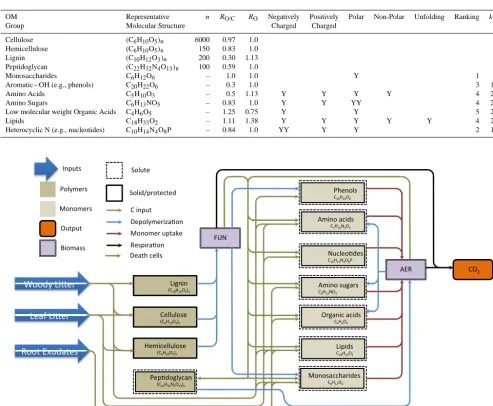
Our approach is to group compounds by quantifiable prop-erties that can be considered to be relevant for metabolic pro-cessing, i.e., oxygen:carbon (O/C) ratio, positive or nega-tive charge, and degree of polarity (Table 1). The rationale behind this strategy is that organic compounds that are al-ready oxidized (as expressed by the O/C ratio) will require less oxygen and lower energy inputs to be fully oxidized to CO2 than more reduced compounds. Polar compounds will be more soluble and thus more mobile in a largely aqueous soil system than non-polar compounds. Ionization state and the sign of an electrical charge are determinants for protec-tive sorpprotec-tive and other interactions with both the mineral ma-trix and charged organic colloids. Our approach is designed to be flexible enough to incorporate other hypotheses regard-ing controls on decomposition and transport such as accessi-bility and aggregation.
The model’s decomposition reaction network consists of four groups of organic compounds: (1) above and be-lowground litter and root exudates; (2) organic polymers; (3) simpler organic monomers; and (4) fungal and bacterial biomass (Fig. 1). Carbon is brought into the system through aboveground litter, belowground litter, and root exudates. Through implicit (i.e., not explicitly represented as a separate pool) exoenzyme activity, the litter can be degraded into sev-eral simpler organics (i.e., monosaccharides, amino sugars, organic acids, amino acids, phenols, lipids, and nucleotides) in proportions that can be manipulated in the model for sen-sitivity analyses (baseline values shown in Fig. 2). Root exu-dates are considered to be simple monomeric organics.
The model assumes fungi and bacteria can assimilate the polymeric and monomeric organics directly, resulting in biomass increases and CO2production. The proportions of compounds that can be assimilated by either microbial pop-ulation are set as baseline values (Fig. 2) and can be manipu-lated in sensitivity analyses. Carbon in microbial necromass is returned to solution (Fig. 1) and can participate in further reactions, be transported vertically, or interact with soil grain surfaces. We parameterized a fraction (fm) of the micro-bial necromass as peptidoglycan, which is intended to rep-resent polymeric cell wall material (Fig. 1). The remaining
necromass carbon is returned to the monomer pools, in pro-portions that can be manipulated for a particular simulation (Fig. 2). Microbial exudation or carbon overflow (Tempest and Neijssel, 1992) from stoichiometric imbalance can be an important contributor to overall microbial carbon turnover in some cases. However, we have not included them in the cur-rent version of the model.
2.3 Decomposition reactions of organic monomers We assume the decomposition of monomers (monosaccha-ride, amino acid, amino sugar, organic acid, lipid, and nu-cleotide) is carried out by aerobic heterotrophic bacteria, which utilize monomers as a source of energy and carbon for biomass growth and maintenance, thus leading to biomass yield and CO2 production. The reaction describing decom-position of 1 mole of generic monomerkC
i, withkcarbon
atoms can be written as follows:
kC
i+RO,i(1−a) kO2→akBA+(1−a) kCO2, (2) where BA (mg C-wet-biomass L solution−1) is the
aero-bic heterotrophic bacteria biomass concentration, a is the assimilation-to-respiration ratio describing the fraction of carbon atoms being assimilated into the cell as compared to the fraction released as CO2, and RO,i is the oxidative
ratio of the compound, which describes the contribution of aqueous O2uptake as compared to the O2available from the substrate. The biomass yield coefficientYi=akforBA
de-scribes the microbial biomass gain per mole of consumed substrate ((g wet-biomass) (mol substrate)−1). The effect of temperature on the decomposition rate was not included in Eq. (2). We leave the determination of an appropriate param-eterization for the temperature effect and related analyses to future work.
2.4 Stoichiometry for fungal depolymerization of organic compounds
Large polymers (represented in this model as cellu-lose (C6HO5)n, hemicellulose (C9H15O7.5)n, and lignin (C10H12O3)n) can be decomposed (depolymerized) into monomers by fungi. The fungi may then assimilate part of the carbon from the substrate polymer, consume O2, pro-duce energy and CO2, and release free monomers available to other microorganisms such as aerobic bacteria. The specific monomer products vary with the source polymer (Fig. 2). A general depolymerization reaction of polymermjC
i, with k
carbon atoms made ofn monomers mjC
j withmj carbon
atoms, is derived from stoichiometric constraints:
mjC
i+RO,i(1−a) kO2→
1−W
P
mjxj
n
(akBF+(1−a) nk)+W X
xjmjCj, (3)
Table 1. Simplified overview of possible molecular functionalities (often dependent on solution pH, monomers only), number of repeating
units for polymers, O/C ratios (R(O/C)), oxidative ratio (RO), and the sorption partitioning coefficient (kfkr) for relevant compound classes.
Y indicates that compound class possesses this particular option to interact with other molecules or surfaces (YY=possesses the option in extraordinary fashion).
OM Representative n RO/C RO Negatively Positively Polar Non-Polar Unfolding Ranking kf/ kr
Group Molecular Structure Charged Charged
Cellulose (C6H10O5)n 6000 0.97 1.0 –
Hemicellulose (C6H10O5)n 150 0.83 1.0 –
Lignin (C10H12O3)n 200 0.30 1.13 –
Peptidoglycan (C22H32N4O13)n 100 0.59 1.0 –
Monosaccharides C6H12O6 – 1.0 1.0 Y 1 700
Aromatic−OH (e.g., phenols) C20H22O6 – 0.3 1.0 3 1400
Amino Acids C5H10O3 – 0.5 1.13 Y Y Y Y 4 2100
Amino Sugars C6H13NO5 – 0.83 1.0 Y Y YY 4 2100
Low molecular weight Organic Acids C4H6O5 – 1.25 0.75 Y Y 5 2400
Lipids C18H33O2 – 1.11 1.38 Y Y Y Y Y 4 2100
Heterocyclic N (e.g., nucleotides) C10H14N4O8P – 0.84 1.0 YY Y Y 2 1100
Pep$doglycan
(C22H32N4O13)n
CO2
Cellulose
(C6H10O5)n
Hemicellulose
(C6H10O5)n
Lignin
(C10H12O3)n
Phenols
C20H22O6
Monosaccharides
C6H12O6
Amino sugars
C6H13NO5
Amino acids
C5H10N2O3
Lipids
C18H33O2
Organic acids
C4H6O5
Nucleo$des
C10H14N4O8P
AER FUN
Biomass Inputs
Solid/protected
Solute
Polymers
Monomers
Output
C input
Depolymeriza$on
Monomer uptake
Respira$on
Death cells
Woody LiRer
Root Exudates Leaf LiRer
Figure 1. Reaction Network Diagram. FUN and AER stand for fungi and heterotrophic aerobic bacteria, respectively.
the fraction of carbon released in the monomers, andxj are
the stoichiometric coefficients in Eq. (2) for each monomer. In Eq. (3), the biomass yield coefficientYiis
Yi=
1−W
Pm
jxj
n
ak. (4)
Note that Eq. (3) can also describe depolymerization reac-tions by exoenzymes (i.e., no direct assimilation and biomass growth) whenW=1 (i.e.,Yi=0).
2.5 Biological reaction rates
The microbial decomposition rate of substrate mjC i is
generically described using Michaelis–Menten kinetics (e.g.,
Maggi et al., 2008):
∂Ci
∂t
d = −µi
Ci
Ki+Ci
O2
KO2+O2
B Yi
f (θ ) g (pH) h (T ) , (5)
where ∂Ci ∂t
i
d is the rate of change of Ci for decomposi-tion (mol m−3s−1); subscript d represents decomposition;
µi (s−1) is the maximum specific consumption rate of
substrate i (s−1) (i.e., the intrinsic decomposition rate); O2 (mol O2m−3)is aqueous O2concentration; B (mg wet-biomass L−1)is biomass of bacteria (BA)or fungi (BF);Yiis
the biomass yield on substratei; andKi andKO2 (mol L
−1)
Source Pool
Destination Pool
ExudatesLeaf Litter
Wood LitterB Death F Death Cellulose
HemiCellulosePeptidoglycan
Lignin
Cellulose Hemicellulose
Peptidoglycan
Lignin Monosaccharaides
Amino Acids Amino Sugars
Organic Acids
Phenols Lipids
Nucleotides
0 0.1 0.2 0.3 0.4
Figure 2. Partitioning of the various carbon source pools into the
eleven SOM destination pools. The values in each column sum to 1.0; each value indicates the fraction of the source pool allocated to a particular destination pool.
environmental effects on microbial activity of soil moisture, pH, and temperatureT, respectively (Maggi et al., 2008). In the current suite of experiments, we did not include the ef-fects of pH or soil water stresses (i.e.,g(pH) andf (θ )are set to 1) on decomposition rates, although these factors can be important (e.g., Schimel et al., 2011). We note that re-cent work has shown that Michaelis–Menten kinetics may be inaccurate when simulating complex consumer-substrate in-teractions (Tang and Riley, 2013), but leave incorporation of these effects into the model for later work.
O2 is consumed during aerobic microbial respiration on monomers and fungal depolymerization (Fig. 1) with rate:
∂O2
∂t
d
=RO,i(1−a)
∂Ci
∂t
d
. (6)
CO2is produced in both reactions with rates that depend on the carbon content in the substrate and the reaction struc-ture. The reaction rates for monomer oxidation and depoly-merization are
∂CO2
∂t
d
= −(1−a)∂Ci ∂t
d
(7)
∂CO2
∂t
d = −
1−W
n
X
mjxj
(1−a) k ∂Ci ∂t
d
, (8)
respectively, whereW is the depolymerization efficiency,k
is the number of carbon atoms in Ci, n is the number of
monomers in the polymer, andmj is the number of carbon
atoms in the product monomerCj.
The decomposer biomass grows as substrate is assimi-lated, and declines as cells die, according to the following:
∂B
∂t = −
n X
i=1
Yi
∂Ci
∂t
d
−δB, (9)
whereδ(s−1)is microbial death rate.
We followed the hypothesis of Kleber (2010) that the O/C ratio (RO/C,i)of relatively simple organic compounds
pro-vides a proxy for the maximum specific consumption rate (Table 2). We fit a simple exponential curve to the observa-tions shown in Fig. 2 of Kleber (2010), and normalized the result to the rate associated with monosaccharides:
µi=
1.15×10⁻¹²s−1 0.006e2.0137RO/C,iµ
Msac. (10) For peptidoglycan, Eq. (10) was not used but a relatively slow intrinsic rate and higher adsorption rate were imposed to represent the tendency of these larger molecules to decom-pose more slowly (Miltner et al., 2012).
2.6 Abiotic processes
CO2gas dissolution is calculated assuming local equilibrium between aqueous and gaseous phases (Maggi et al., 2008). Diffusivities are estimated based on the molecular weight of each component and the Millington and Quirk (1961) ap-proach to account for tortuosity. Water flow is modeled using the Darcy–Richards equation (Pruess et al., 1999) and the van Genuchten (1980) relationships for matric potential and hydraulic conductivity with soil water saturation. Advective gaseous transport as a result of pressure gradients was not considered in the present study, although it can be included using the equations of states available in the TOUGHREACT standard features.
Adsorption and desorption are complex processes that de-pend on characteristics of the organic molecules, soil mineral surfaces and properties, and aqueous chemistry (Dudal and Gerard, 2004). Further, there are large differences in temper-ature sensitivities for the various sorption mechanisms (Co-nant et al., 2011), motivating explicit representation of these processes in models. To examine the impact of sorption on predicted SOM stocks, we imposed forward (adsorption;kf (s−1))and reverse (desorption;k
r(s−1))rates. In the absence of competing sources and sinks of a particular species, this formulation would result in an effective equilibrium linear sorption relationship:Kd=kf/ kr. In our formulation, sorp-tion reacsorp-tions are subsumed in theP
m ∂Ci
∂t
mterms of Eq. (1),
kfis taken to be 6.6×10⁻⁸s−1, and sorbed species are pro-tected from decomposition.
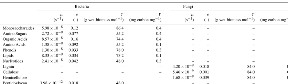
Table 2. Parameters defining decomposition of organic matter pools by bacteria and fungi for maximum specific consumption rate (µ), assimilation-to-respiration ratio (α), and yield (Y).
Bacteria Fungi
µ e Y Y µ e Y Y
(s−1) (–) (g wet-biomass mol−1) (mg carbon mg−1) (s−1) (–) (g wet-biomass mol−1) (mg carbon mg−1)
Monosaccharaides 5.98×10⁻⁸ 0.12 86.4 0.4 – – – –
Amino Sugars 2.72×10⁻⁸ 0.077 55.2 0.4 – – – –
Organic Acids 8.57×10⁻⁸ 0.16 74.4 0.4 – – – –
Amino Acids 1.38×10⁻⁸ 0.092 55.2 0.1 – – – –
Phenols 1.30×10⁻⁸ 0.033 78.0 0.3 – – – –
Lipids 8.33×10⁻⁹ 0.034 73.2 0.1 – – – –
Nucleotides 2.41×10⁻⁸ 0.042 48.0 0.3 – – – –
Lignin – – – – 4.20×10⁻⁹ 0.018 84.0 0.5
Cellulose – – – – 5.46×10⁻⁹ 0.001 84.0 0.5
Hemicellulose – – – – 1.68×10⁻⁸ 0.039 84.0 0.5
Peptidoglycan 3.98×10⁻¹² 0.018 48.0 – – – –
closely follows a Langmuir relationship than a linear rela-tionship. We note that both of these approaches assume equi-librium between the sorbed and aqueous phases, although the Langmuir relationship implies a partitioning dependent on soil properties and the sorbed concentration. We intend to examine the impact of the functional form of the sorption isotherm on SOM dynamics in future work.
Soil aggregation (Six et al., 2001, 2004) is another impor-tant process that can lead to carbon persistence in soil. The density of aggregates and rates of aggregation and disaggre-gation in soil depend on many ecosystem properties (Conant et al., 2011), so properly representing their impacts on pro-tected SOM may be important in climate change studies. Al-though important for SOM residence times, the density of aggregates and rates of aggregation and disaggregation have not yet been represented in the model.
2.7 Climate forcing, boundary conditions, and initial conditions
Climate forcing (precipitation, evapotranspiration, temper-ature) and carbon inputs used in the BAMS1 simulations were taken from a CLM4 (Lawrence et al., 2011) simula-tion of a US Great Plains grassland. CLM4 is the land model integrated in the Earth system model called CESM1 (http: //www.cesm.ucar.edu/models/cesm1.0/), and represents sur-face and subsursur-face hydrology, ecosystem energy exchanges with the atmosphere, and plant and soil biogeochemistry. The equilibrium simulations for comparison to SOM obser-vations were forced with repeated 1948–1972 cycles from Qian et al. (2006). For the BAMS1 simulations, we imposed the CLM4 predicted infiltration and carbon inputs from leaf, wood, and root litter partitioned into the soil using expo-nentially decaying depth profiles with length scales of 1, 7, and 12 cm, respectively. Baseline simulations were run for 10 000 years from initial conditions of no soil carbon and for constant climate forcing. This spin-up period was sufficient
to ensure that overall changes in SOM stocks were less than 0.01 % yr−1by the end of the simulation.
Having a fully coupled model that includes reactive trans-port capabilities and the aboveground process representa-tions in CLM4 would be the preferred model structure to perform the analyses we are presenting here because it would allow for the coupling between above and belowground pro-cesses. However, to our knowledge such a capability does not currently exist (although efforts are underway, e.g., Tang et al., 2013).
2.8 Comparison to SOM and114C observations In this work we were primarily interested in exploring hy-potheses that could explain variations in SOM residence times; therefore, our comparisons to SOM observations were designed to engender confidence that the suite of processes we have included were internally consistent and produced re-alistic SOM predictions, but not that they describe precisely the conditions and SOM profiles of a specific site. We there-fore compared the predicted SOM profiles using the baseline set of parameters to observations from grasslands located be-tween 39◦N and 43◦N latitude across Nebraska and Col-orado. Compiled vertically resolved observations of SOM content from the National Soil Carbon Database (NSCN; available at http://www.fluxdata.org/nscn/SitePages/Home. aspx) included 618 observations in that region; Fig. 3). Along with SOM profiles, root profiles from grasslands in the same region were selected from the Global Root Distribution Pro-file database (Schenk and Jackson, 2005).
0
0.2
0.5
1
2
0 0.005 0.01 0.015 0.02 0.025 0.03
Depth [m]
Total SOM (kg
C kg −1 soil)
Predicted Observed
Figure 3. Predicted and observed SOM content. Observed values
are represented as average and standard deviation of 618 observa-tions from grasslands extracted from the NSCN database.
SOM radiocarbon (114C) profiles are potentially valuable tracers of the integrated suite of processes affecting verti-cal SOM profiles and have recently been applied to evaluate climate-scale land surface model SOM predictions (Jenkin-son and Coleman, 2008; Koven et al., 2013). We predicted SOM114C values in the year 2003 by running a parallel sim-ulation to the bulk SOM simsim-ulation, but imposing a first order decay term (with turnover time of 8267 year corresponding to the14C radioactive decay rate) for each modeled compo-nent in both aqueous and protected phases. To impose the “bomb” atmospheric 14C content, we applied the northern hemispheric values from Levin and Hesshaimer (2000) for 1950–1976 and Levin and Kromer (2004) for 1977–2003. 2.9 Model analyses
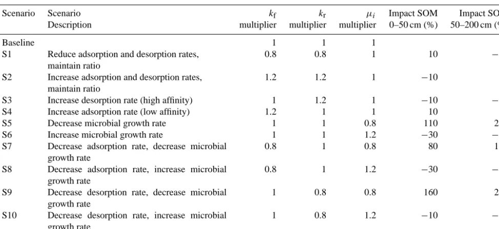
We performed ten sensitivity tests (Table 3) and a number of model experiments to explore how system properties and changes in soil microclimate may impact SOM dynamics. To investigate the relative importance of adsorption and des-orption rates from soil mineral surfaces on equilibrium SOM stocks, we performed simulation scenarios varying the sorp-tion rateskfandkr(Table 3). First, we modifiedkfandkr con-currently by factors of 0.8 (S1) and 1.2 (S2) (resulting in an unchanged value ofKd). Next, we investigated the impacts of the different temperature sensitivities of desorption and adsorption. As noted in Conant et al. (2011), warmer tem-peratures favor desorption for high-affinity soil OM–mineral interactions (e.g., non-covalent bonds) and favor adsorption for low-affinity soil OM–mineral interactions. For sensitiv-ity analyses S3 and S4, we assumed a mean temperature in-crease throughout the profile that led to a relative inin-crease in desorption (kr)of a factor of 1.2 (S3; high affinity) and
a relative increase in adsorption (kf)of a factor of 1.2 (S4; low affinity). Although this sensitivity analysis substantially under-represents the complexity of the temperature depen-dencies of sorption and protection mechanisms, it does al-low us to qualitatively investigate the impact of temperature-dependent sorption on vertically resolved SOM content. We note that protection associated with occlusion and aggrega-tion will also have temperature sensitivities (Conant et al., 2011); we did not analyze those affects here.
We also manipulated the microbially mediated transfor-mation rates by multiplyingµi by factors of 0.8 (S5) and
1.2 (S6). Because interactions between sorption and the frac-tion of each compound accessible to decomposifrac-tion (i.e., in the aqueous phase) will impact SOM content, we performed perturbations toµi in combination with perturbations tokf andkr(scenarios S7, S8, S9, and S10). Total SOM profiles for these scenarios were again compared to the baseline sce-narios. For all the sensitivity analyses we also estimated the
114C SOM vertical profile.
To further examine carbon and microbial dynamics in the system, we performed an experiment with two 500-year ulations, both starting from the end of the 10 000-year sim-ulation. The first simply continued the 10 000-year simula-tion for an addisimula-tional 500 years. In the second simulasimula-tion, we doubled all chemical species initial concentrations in the top 20 cm from those at the end of the 10 000-year simulation, and performed a 500-year simulation. Differences between these simulations over the 500-year period were used to in-vestigate coupled C, microbial, and transport dynamics.
Table 3. Description of parameters and mechanisms used in the sensitivity analysis. The three multipliers indicate the factors applied to the
parameter for each sensitivity scenario. The last two columns indicate the impacts of each sensitivity scenario parameter changes on 0–50 cm and 50–200 cm total SOM contents.
Scenario Scenario kf kr µi Impact SOM Impact SOM
Description multiplier multiplier multiplier 0–50 cm (%) 50–200 cm (%)
Baseline 1 1 1
S1 Reduce adsorption and desorption rates, maintain ratio
0.8 0.8 1 10 −10
S2 Increase adsorption and desorption rates, maintain ratio
1.2 1.2 1 −10 0
S3 Increase desorption rate (high affinity) 1 1.2 1 −10 −10 S4 Increase adsorption rate (low affinity) 1.2 1 1 10 0 S5 Decrease microbial growth rate 1 1 0.8 110 220 S6 Increase microbial growth rate 1 1 1.2 −30 −50 S7 Decrease adsorption rate, decrease microbial
growth rate
0.8 1 0.8 80 190
S8 Decrease adsorption rate, increase microbial growth rate
0.8 1 1.2 −30 −50
S9 Decrease desorption rate, decrease microbial growth rate
1 0.8 0.8 160 240
S10 Decrease desorption rate, increase microbial growth rate
1 0.8 1.2 −10 −40
3 Results
3.1 Equilibrium predictions for the grassland sites Using the baseline set of parameters (Table 2), climate, car-bon inputs, and a 10 000-year simulation, the model esti-mated total SOM contents roughly in agreement with the grassland observations we compiled (Fig. 3). At steady state, most of the input polymers (cellulose, hemicellulose, lignin) were predicted to be in the top meter of soil (Fig. 4a), con-sistent with the depth-distribution of the source carbon and the assumed inability of protected-phase compounds to move vertically. Lignin had the largest concentration of the input polymers, with a peak at about 10 cm depth. The fraction of total SOM predicted to be lignin was highest (∼1–2 %, as compared to more than 20 % for leaf and root C inputs) in the zone where direct carbon inputs occurred and decreased to ∼0 % by 1 m depth (Fig. 5b). The mean predicted pro-portion was about 1 % between 0 and 50 cm depth and com-pared well with the values from the synthesis by Thevenot et al. (2010), who reported a range for grasslands of∼ 0.7– 2.7 %. Cellulose and hemicellulose concentrations had flatter vertical concentration gradients and levels about an order of magnitude lower than that of lignin.
Monomers protected (sorbed) on surfaces (Fig. 4b) had a deeper concentration profile than the input polymers, con-sistent with their ability to partition into the aqueous phase and move vertically with water advection and through dif-fusion. Of the sorption-protected monomers, the predicted relative concentration ranking, from highest to lowest, was monosaccharides, amino acids, lipids, phenols, and organic
acids. Very little amino sugars or nucleotides were predicted to persist in the protected phase.
The vertical profile shape of the predicted total dissolved monomer content was similar to that for protected-phase monomers, while the relative abundances were 2–3 orders of magnitude lower (Fig. 4c). Dissolved monosaccharides had the highest predicted concentrations, followed by amino acids, lipids, phenols, and organic acids. The other dissolved monomers were predicted to have much lower concentra-tions.
The proportion of total microbial biomass predicted to be fungal was largest at the surface and declined rapidly to ∼0 % at 40 cm depth (Fig. 5a), consistent with the expecta-tion that fungi inhabit the porexpecta-tion of the soil column domi-nated by recent plant carbon inputs and the few observations available for comparison (Ekelund et al., 2001; Zhou et al., 2008).
3.2 Sensitivity analysis for total SOM
0.5
1
1.5
2
0 1 2
x 10−4 Polymer Inputs (kgC kg−soil1)
Depth (m) Cellulose
Hemicellulose Lignin
0.5
1
1.5
2
0 0.005 0.01 0.015 0.02
Protected (kg C kg
−1
soil)
Depth (m)
Monosaccharaides Amino Acids Amino Sugars Organic Acids Phenols Lipids Nucleotides Peptidoglycan
0.5
1
1.5
2
0 0.2 0.4 0.6 0.8 1
x 10−5 Dissolved (kg
C kg
−1
soil)
Depth (m)
Monosaccharaides Amino Acids Amino Sugars Organic Acids Phenols Lipids Nucleotides
Figure 4. Predicted steady state (a) protected-phase polymers; (b) protected-phase monomers; and (c) dissolved monomers as a
function of depth after 10 k year of simulations in the grassland.
a factor of 1.2 increase in desorption rates (S3) and factor of 1.2 increase in adsorption rates (S4) (Fig. 6a). These changes also had very small impacts on predicted SOM content.
Modifying the bacterial SOM consumption rates (µi)on
all aqueous compounds by factors of 0.8 (S5) and 1.2 (S6) had relatively larger impacts on SOM content (Fig. 6b). As expected, decreasingµi led to increased SOM contents,
while increasingµi led to lower SOM contents throughout
the soil column. As discussed below, these changes highlight the potential impacts of a temperature-dependent microbial growth rate.
Finally, modifying kf, kr, and µi concurrently also had
large impacts on SOM (Fig. 6c). Decreasing kf andµi
si-multaneously (S7) led to increases in both 0–50 cm and 50– 200 cm SOM content that were comparable (but slightly smaller) to those from S5 (which only decreased µi).
De-creasing kf and increasing µi simultaneously (S8) led to
about a 30–50 % reduction in SOM, consistent with the im-pact of increasingµi alone and the very small impact of
de-creasingkfalone. Decreasingkrandµi simultaneously (S9)
resulted in large increases in SOM throughout the column. Finally, decreasingkrand increasingµi (S10), which alone
0 1 2 3
Lignin (% SOM) (b)
0 5 10
0
0.2
0.4
0.6
0.8
1
Fungi (% Biomass)
Depth (m)
(a)
Figure 5. Proportion of biomass that is fungal (a) and proportion of
total SOM that is lignin (b) as functions of depth.
have opposite impacts, led to a moderate decrease in SOM content. In these sensitivity scenarios, the impacts of changes in microbial growth rate dominated the impacts from changes in sorption parameters.
3.3 Sensitivity analysis for114C of total SOM
The baseline simulation resulted in114C profiles in soils that had a qualitative shape (i.e., monotonic depletion with depth) and values at depth consistent with observations (Fig. 6d), although the near-surface values were too depleted com-pared to the few observational data sets published for grass-lands. We discuss potential reasons for this mismatch be-low, but note here that we did not attempt to tune a sepa-rate non-equilibrium pool near the soil surface that would al-low for a better match with this expectation. We expected the
114C value at about 1 m depth to be in the range [−600 ‰, −400 ‰], based on pasture and grassland observations at Paragominas, Brazil (Trumbore et al., 1995) and Riverbank, California and Judgeford, New Zealand (Baisden and Parfitt, 2007).
For scenarios S1, S2, S3, and S4, the predicted changes in the114C value of total SOM at 1 m depth were between ∼0 and−80 ‰. Using a simple one-box donor-controlled turnover model (i.e., first order loss) implies that the14 C-inferred changes in turnover times between, e.g., S1 and the baseline simulations at 50 cm depth, were relatively larger than those predicted for the total SOM content changes (33 % versus 7 %, respectively). This pattern was consistent across scenarios S1, S2, S3, and S4 for all depths. Decreasing the microbial growth rate (µi; S5) and increasingµi (S6) while
holding all other parameters constant led to enhanced de-pletions of about 50 ‰ in 114C below about 0.5 m depth (Fig. 6e). Scenarios S7–S10 all led to enhanced14C deple-tion compared to the baseline (Fig. 6f), with the largest en-hanced depletion (∼100 ‰) corresponding to S9 (decreasing
0
0.5
1
1.5
2
0 0.01 0.02 0.03
Depth (m)
Total SOM (kg
C kg
−1
soil)
(a)
Observed Baseline S1; kf (−); kr (−) S2; kf (+); kr (+) S3; k
r (+) S4; kf (+)
−600 −400 −200 0
0
0.5
1
1.5
2
Depth (m)
Δ14C SOM (o/
oo)
(d) 0
0.5
1
1.5
2
0 0.01 0.02 0.03
Total SOM (kg
C kg
−1
soil)
(b)
Observed Baseline S5; μi (−) S6; μi (+)
−600 −400 −200 0
0
0.5
1
1.5
2
Δ14C SOM (o/
oo)
(e) 0
0.5
1
1.5
2
0 0.01 0.02 0.03
Total SOM (kg
C kg
−1
soil)
(c)
Observed Baseline S7; kf (−); μi (−) S8; k
f (−); μi (+) S9; k
r (−); μi (−) S10; kr (−); μi (+)
−600 −400 −200 0
0
0.5
1
1.5
2
Δ14C SOM (o/
oo)
(f)
Figure 6. Total SOM content (top row) and114C of total SOM (bottom row) at end of 10 000-year simulation for the ten sensitivity scenarios
(a and d: S1–S4; b and e: S5–S6; c and f: S7–S10) that varied combinations ofkf,kr, andµi(Table 3).
µi)and the smallest (∼30 ‰) to S7 (decreasingkfandµi)
and S8 (decreasingkfand increasingµi).
3.4 Transient pulse experiments
We performed several transient pulse experiments to inves-tigate SOM turnover dynamics, vertical transport, and effec-tive turnover times of the various compounds in the system. First, we applied a pulse of all compounds by doubling the initial concentrations in the top 20 cm of the soil column and performing a 500-year simulation starting with conditions from the end of the 10 000-year baseline simulation. Concen-tration differences compared to a 500-year simulation with baseline parameters (i.e., effectively continuing the 10 000-year spin-up simulation another 500 000-years) varied widely be-tween the various simulated carbon compounds (Fig. 7). The anomalies are shown as log10transformations of the absolute % differences from the baseline 500-year simulation; nega-tive anomalies are indicated by white contours.
Anomalies in cellulose and hemicellulose were 0.01– 0.1 % in the top 5 cm of soil and persisted for the entire simu-lation. Negative anomalies (i.e., priming) were predicted be-tween about 10 and 20 cm out to about 300 years. Lignin anomalies in the top 5 cm of soil had similar patterns to cel-lulose, but in contrast the positive perturbation of about 1 % below about 5 cm persisted for decades. Both aerobic bacte-ria and fungi were predicted to have∼10 % increases in the
top 20 cm of soil shortly after the perturbation, and these in-creases were predicted to persist for many decades. It appears that the microbial biomass has moved into another relatively persistent state.
The largest anomalies in protected monomers were pre-dicted in the amino acids, amino sugars, phenols, and lipids pools, all of which showed perturbations of about 10 % in the top 20 cm of soil for hundreds of years. Beyond the poly-mer species, only the monosaccharides and organic acids were predicted to have negative anomalies, and the mag-nitudes of these anomalies were relatively small (less than ∼1 %). Anomalies in total SOM were predicted to be∼1 %, 0.1 %, and 0.01 % in the 0–10, 10–100, and 100–200 cm depth ranges, respectively, by the end of the 500-year sim-ulation.
Depth (m)
B aerobic 0
1
2 −0.5
0 0.5
B fungi 0
1
2 −2
−1 0
Cellulose 0
0.5
−2 −1 0
Depth (m)
Hemicellulose 0
0.5
−2 −1 0
Lignin 0
0.5 −2
−1 0
Monosaccharides 0
1
2 −2
−1 0 1
Depth (m)
Amino Acids 0
1
2
−2 0 2
Amino Sugars 0
1
2
−2 0 2
Organic Acids 0
1
2 −2.5
−2 −1.5 −1 −0.5
Depth (m)
Phenols 0
1
2
−2 0 2
Time (y) Lipids
0 200 400
0
1
2
−2 0 2
Time (y) Nucleotides
0 200 400
0
1
2
−2 0 2
Time (y)
Depth (m)
SOM
0 200 400
0
1
2 −2.5
−2 −1.5 −1 −0.5
Figure 7. Time and depth profiles of microbial and chemical species concentration anomalies (log10( %|anomaly|) compared to the baseline
simulation) for the perturbation experiment that doubled all chemical species concentrations in the top 20 cm of soil as an initial condition. To highlight important features, we: (1) used different ordinate axes for cellulose, hemicellulose, and lignin; (2) excluded anomalies less than 0.001 %; and (3) used solid filled contours where the anomalies were positive and white contour lines surrounding regions where the anomalies were negative (e.g., for the monosaccharides below about 20 cm after about 200 years).
years associated primarily with rapid microbial responses and advective transport. We applied a first-order approxi-mation to estimate the turnover time (τ )for total SOM and DOM anomalies to re-equilibrate as a function of the depth interval of the perturbation (Fig. 8c).
The SOM and DOM turnover times followed the same qualitative pattern with depth: a slight increase from an inter-mediate value down to 30 cm, an increase to about 1 m, and then a relatively constantτ below 1 m. However, the DOM
τ was always lower than the total SOMτ, with the ratio be-tween them being∼100 down to∼70 cm and a ratio of∼3 below∼70 cm. Turnover times estimated from the radiocar-bon profiles show modest coherence with the pulse-based es-timates for total SOM, but much higher turnover times for DOM dynamics.
4 Discussion
4.1 Model predictions
0 1 2 3 0
0.1 0.2 0.3 0.4 0.5 0.6 0.7 0.8 0.9 1
Time (y)
Scaled SO
M
and DO
M
Anomalies
(a)
SOM = Solid DOM = Dashed
0−10 cm 10−20 cm 20−30 cm 30−40 cm 40−75 cm 75−125 cm 125−200 cm
102 0
0.1 0.2 0.3 0.4 0.5 0.6 0.7 0.8 0.9 1
Time (y)
Scaled SO
M
and DO
M
Anomalies
(b)
SOM = Solid DOM = Dashed
0−10 cm 10−20 cm 20−30 cm 30−40 cm 40−75 cm 75−125 cm 125−200 cm
100 101 102 103 104 0−10 cm
10−20 cm
20−30 cm
30−40 cm
40−75 cm
75−125 cm
125−200 cm
Inferred Turnover Time (y)
Depth Interval
(c)
From Total SOM From Total DOM From 14C of Total SOM
From 14C of Total DOM
Figure 8. (a, b) Predicted 5000 year time histories of the scaled total SOM and total DOM anomalies resulting from a doubling of all
compounds in the specified depth intervals (a shows first 3 years on a linear time scale and b shows 3–5000 years on a log time scale).
(c) Inferred first-order turnover times and14C ages for total SOM and total DOM as a function of depth interval following the perturbation.
the 114C values (Fig. 8c). The prediction that total DOM concentrations were three orders of magnitude lower than protected-phase SOM concentrations (Fig. 4) is consistent with observations of a vertisol grassland (Don and Schulze, 2008), mollisol grassland, and ultisol forest sites (Sander-man et al., 2008). However, DOM concentrations are much more variable than SOM, so this ratio is not in general a good metric for comparison with model predictions. Com-bining all the dissolved monomer concentrations with the water flux through the system resulted in a predicted annual DOM leaching flux of 6.2 g m−2year−1, which matches very well the estimate by Kindler et al. (2011) for grasslands of 5.3±2 g m−2year−1.
The role of microbial cell wall components as stable car-bon compounds in soils has been discussed in several recent articles (e.g., Clemente et al., 2012). In the reaction network developed here, the compound we assigned to represent cell wall material (peptidoglycan) accounted for 5–10 % of SOM at steady state; this is a large enough fraction of SOM that resolving uncertainty in the partitioning of new microbial necromass into different species would be very useful.
Different model structures have reproduced observed de-creases in SOM content with depth in a variety of ecosystems (Jenkinson et al., 2008; Koven et al., 2011, 2013; Tang et al., 2013). However, because there are many ways that multiple-pool SOM models can be calibrated against bulk SOM obser-vations, we do not take the match of our vertical profile SOM content predictions with observations (Fig. 3) to be a particu-larly strong validation of our model structure. Since so many different model structures and parameterizations can match bulk SOM observations, the development of clear falsifiable
hypotheses for these observed patterns remains an important goal for SOM model development.
Vertical profiles of114C values of total and dissolved or-ganic carbon are a valuable constraint on process represen-tation in SOM dynamics models. Although we did not sim-ulate a particular site with 114C observations, our predic-tions are consistent with the general structure of a mono-tonic decrease in114C value with depth to values less than −400 ‰ by∼1 m depth. The decreasing114C values with depth occur because of a decrease in the decomposition rate with depth associated with decreasing substrate concentra-tions and therefore microbial biomass, rather than transport times from the surface, as also seen in sensitivity analyses in Koven et al. (2013). Over time, the accumulation of material on the mineral surfaces and14C decay leads to a relatively
114C depleted SOM profile at depth.
of modest size (Fig. 3), and effectively not in equilibrium with the aqueous phase, can explain the bias between our predicted and commonly observed114C values near the soil surface. Our model allows for an additional non-equilibrium carbon pool that could be tuned to match these 114C and SOM profiles, but we have avoided that type of tuning here. Processes that may be good candidates for this level of pro-tection include aggregation and formation of colloids, which have been shown to substantially affect chemical mobility and carbon decomposition rates in soils (Daynes et al., 2013; Kausch and Pallud, 2013; Six et al., 2000). Development of process representations that will improve these comparisons is a task we leave for future research.
Other mechanisms not currently included in our model have also been hypothesized, and in some cases demon-strated, to play a role in the dynamics of deep SOM and its relatively depleted 114C values. First, because the relative abundance of substrates at depth is low, physical separation between microbes and substrates could limit decomposition rates (Chabbi et al., 2009; Ekschmitt et al., 2008). The in-accessibility of substrates is expected to increase nonlinearly with soil drying. Models for this particular mechanism have been proposed by considering the effective diffusivity of sub-strate material as a function of pore geometry and moisture content (Or et al., 2007). Second, the density of mineral sorp-tion sites increases with depth, which can lead to an effective inhibition of exoenzyme activity as these enzymes interact with mineral surfaces instead of substrate (Quiquampoix et al., 2002; Tietjen and Wetzel, 2003). Third, on the long time scales that we have simulated here, bioturbation may be an important vertical mixing mechanism, although it has been shown to be negligible in a forest soil (Braakhekke et al., 2013). As a final example, formation of aggregates that ef-fectively shield SOM from decomposition could also play a role in some soils (see the review by Six et al., 2004).
Characterizing model structural uncertainty requires a more complete set of observational metrics that are specific to the model structure being tested. For a Century-like model without observationally defined pools, even with carefully constrained carbon inputs, one can only compare modeled and observed total SOM content and114C values. But, since specific combinations of SOM content and 114C values in these types of models can be achieved with various combi-nations of parameters (Jenkinson and Coleman, 2008; Koven et al., 2013), and since the carbon content and 114C value of modeled individual pools cannot be measured separately, it is difficult to tell if the partitioning of carbon between pools, vertical transport of material, and protection mecha-nisms were properly represented. This particular problem is partly alleviated in a model like the one described here; the problem then becomes finding observations of the specific carbon compounds and their partitioning between phases. More generally, modeling mechanisms or pools that can be approximated by measured quantities should enable much more informative testing and model development.
An additional technique to assess model structural uncer-tainty would be that of building a set of increasingly simpli-fied models based on the one presented and analyzed here, and then comparing their goodness of fits against existing metrics after parameter estimation. We did not apply such an approach here since we did not have sufficient observa-tions from one specific site, but could only assess model per-formance against trends from heterogeneous observations. However, testing model structural uncertainty will be per-formed in future work to gain confidence in the model struc-ture and to inform the level of complexity required for a par-ticular application.
4.1.1 Sensitivity analyses
Our sensitivity analyses were designed to better understand system dynamics and to highlight areas of uncertainty that could motivate future observations. We found that uncer-tainty in sorption rates (S3, S4; Fig. 6), designed to mimic sorption sensitivity to warming, had only a small effect on total-column SOM after 10 000 years. Of course, SOM dy-namics under decadal-scale climate change will be influ-enced by many different temperature dependencies and their interactions.
Microbial growth rates had asymmetric impacts on SOM profiles. In particular, increased microbial growth rates (S6) decreased SOM content to a lesser degree than decreased growth rates (S5) increased SOM content. These scenarios both led to more114C depleted total SOM compared to the baseline, but with a larger decline associated with increased growth rates. Even though the high-growth scenario (S6) had less stabilized SOM at depth than scenario S5, the increased microbial growth rates led to about a doubling of peptido-glycan (i.e., microbial cell wall residuals after death) levels compared to the baseline. These compounds were strongly adsorbed and had low reactivity, thus they had relatively de-pleted114C values compared to the other protected species and resulted in14C depletion of the total SOM pool.
In the experiments manipulating sorption rates (kf,kr)and microbial growth rate (µi), all four combinations led to SOM
contents mostly outside the standard deviations of the obser-vations. The largest biases were associated with both des-orption and intrinsic microbial growth rates being simultane-ously decreased (S9). Both scenarios that increased the mi-crobial growth rate (S8, S10) led to low SOM content and all four scenarios led to more depleted SOM114C values as compared to the baseline simulation.
4.1.2 Pulse experiments
a relatively long memory in this dynamic system. In a real system with continuously or seasonally pulsing inputs, such a signal would be indistinguishable after a few carbon-input pulses. Some of the chemical species’ had negative anoma-lies from the baseline that only manifested several decades after the perturbation. Although these anomalies were rel-atively small compared to the perturbation, they show that the overall system responses can have interesting transients and other complexities. Critically, the intrinsic rates affecting carbon turnover that are integrated in the model are faster than the overall system response characteristic time. Thus, the prediction that the total SOM characteristic response time is longer than these intrinsic rates indicates a substantial amount of recycling of carbon species between the aqueous, microbial, and protected pools.
The pulse injection experiment, where SOM was in-jected and followed for 5000 years, also showed relatively longer total SOM (∼100–300 years) and shorter DOM (0.5– 10 years) simplified first-order turnover times down to about 30 cm (Fig. 8c). The decrease, and then increase, in turnover times with depth for this transient case is different than that inferred from our predictions of a monotonically decreasing
114C profile of DOM and total SOM at steady state (Figs. 6d and 8c). This discrepancy highlights the differences in inter-pretation of SOM turnover rates based on the metric used to characterize turnover. Further, there appear to be at least two characteristic turnover times each for DOM and SOM in the pulse experiments:∼ 1 year (Fig. 8a) and >100 years (Fig. 8b).
4.2 Development of new SOM models
The model structures introduced by the Century (Parton et al., 1987) and RothC (Jenkinson and Coleman, 2008; Jenk-inson et al., 2008) models include several SOM pools with pre-assigned turnover times that are modified by soil temper-ature, soil moisture, and soil texture. In that class of models, the input path of carbon to the various SOM pools may de-pend on the input lignin content, soil texture, or other ecosys-tem properties. Those models depend on the wide range in imposed SOM turnover times (months to centuries) to make equilibrium predictions consistent with observations, yet it is not possible to explicitly measure or identify the groups of compounds existing in any of the assumed pools. Further, several important aspects of that model structure have been challenged based on recent analyses using fine-resolution vi-sualization (e.g., Lehman et al., 2008), molecular character-ization (e.g., Kleber et al., 2010), field studies (e.g., Torn et al., 1997), and isotopic probes (e.g., Gleixner, 2013).
Because existing models do not represent many of the ecosystem processes that have strong climate dependencies, predictions of global terrestrial carbon cycle responses to climate change over the next century may be substantially in error. This contention is supported by recent analyses of Earth system model predictions (Todd-Brown et al., 2013).
We believe that the (1) recognition that important climate-relevant processes are missing from land models; (2) impor-tance of terrestrial carbon dynamics on atmospheric green-house gas levels and climate; and (3) poor performance of these ESMs with respect to SOM dynamics, all argue for a re-evaluation of the methods used to predict carbon dynamics in land models.
Over the past decade, there have been major changes in the conceptual framework of SOM dynamics, evolving from one of carbon pools defined by assumed characteristic turnover times, to one in which organic material is cycled among pools of different physical-chemical state (such as adsorbed to a mineral surface or occluded in an aggregate) with turnover times primarily determined by the interaction of microbial and physical-chemical factors. This move away from a re-liance on intrinsic recalcitrance to explain dynamics follows a parallel new understanding that soil organic matter com-prises only a small amount of selectively preserved plant in-puts and is composed more of microbial necromass and rel-atively simpler organic molecules with higher intrinsic de-composability (Miltner et al., 2012). The observed longevity, quantity, and vertical distribution of SOM profiles are insistent with a high level of decomposability, and are con-sidered to be the result of various protection mechanisms (e.g., mineral interactions, aggregation), physical separation of substrates and their consumers, microbial population dy-namics and activity (Allison et al., 2010; Lawrence et al., 2009; Tang and Riley, 2013; Wang et al., 2013), and trans-port mechanisms (Sanderman and Amundson, 2008). Since these mechanisms have different soil temperature and mois-ture sensitivities, have different characteristic temporal and spatial scales, and affect the various components of SOM dif-ferently, characterizing the impact of any single mechanism on emergent, vertically resolved SOM dynamics is difficult without a model capable of representing this coupled system. The model structure proposed here is a start toward devel-oping that type of process representation. Many other pro-cesses could also be included for a robust assessment of the emergent system behavior of soils under changing climate, changing vegetation type and status, and spatially varying soils, hydrology, and vegetation properties.
transport of colloids (Flury and Qiu, 2008; Thompson et al., 2006); (c) surface interactions (Conant et al., 2011); (d) en-zyme dynamics (Allison et al., 2010); (e) nutrient–microbe interactions; (f) microbe-plant interactions; and (g) represen-tation of subgrid-scale heterogeneity in soil properties and climate.
We propose that a new modeling methodology is needed that uses observations to improve explicit representation of the relevant processes while characterizing uncertainty and avoiding parameter equifinality (i.e., multiple parame-ter value-combinations resulting in a comparable match to the emergent-scale observations; Tang and Zhuang, 2008). In our study, moderate parameter perturbations caused large changes in predicted profile SOM content (Fig. 6), highlight-ing the value of coherent observational data sets that can be used to better constrain model parameter estimation and test model predictions (Moorhead et al., 2013). Although we argue for a more complex model structure to represent the many processes affecting SOM dynamics, the resulting system complexity makes determining individual parameter values difficult, especially if only observations of the emer-gent properties and behaviors of the system are used. For example, it has been common practice to use surface CO2 flux measurements to infer temperature sensitivity of het-erotrophic respiration. However, a careful analysis of the ver-tically resolved temperature and CO2 production indicates that such an approach may be overly simplistic (Gu et al., 2004; Phillips et al., 2013; Tang and Riley, 2013).
For parameter calibration in a complex SOM model, it may be useful to use observations that target a specific mech-anism under controlled conditions. For example, laboratory sorption experiments could be carried out in sterilized soil with known aqueous composition and temperature. Control-ling observations in this manner reduces the influence of other processes (e.g., plant inputs, microbial decomposition, bulk transport), but we also recognize that laboratory exper-iments have artifacts and rates tend to be much faster in the laboratory than in situ. Uncertainty in the parameter values should be propagated through the remainder of the full model (Luo et al., 2009) and tested under relatively controlled field conditions. With careful calibration and uncertainty charac-terization, confidence in the coupled model predictions is en-hanced or, if the total-system uncertainty is large, submodels that significantly reduce predictability could be identified for further work. Finally, such an uncertainty quantification and parameter estimation framework could also inform the level of complexity required to answer a particular question. 4.4 Application to regional- and climate-scale models As with almost all soil biogeochemistry models, we have only applied the model introduced here in a one-dimensional column, but terrestrial ecosystems have spatial heterogene-ity that affect SOM dynamics in edaphic properties (Bird et al., 2002), soil moisture (Riley and Shen, 2014; Sivapalan,
2005) and temperature (Davidson and Janssens, 2006), veg-etation (Turner et al., 2004), and so on. While spatial vari-ability in SOM dynamics occurs at scales from pore (King et al., 2010; Molins et al., 2012) to meters (Frei et al., 2012; King et al., 2010; Mishra and Riley, 2012) to km (Li et al., 2008), in climate models (typical resolution∼100 km) the spatial heterogeneity in ecosystem properties is typically rep-resented by spatially non-specific tiling of, e.g., plant func-tional types (Lawrence et al., 2011). In the absence of al-ternatives, it is often taken as an article of faith that single-column representations of SOM dynamics can be spatially scaled by simple area averaging, but whether this approach gives a reasonable approximation to existing or future SOM stocks is not well tested. Addressing this question will re-quire a suite of modeling approaches combined with finely resolved observations. In the modeling context, we contend that it is important to represent the underlying mechanisms of SOM dynamics at the spatial resolution at which they can be observed, at least in benchmark or exploratory models. It is unlikely, however, that a robust three-dimensional reactive transport solver will be developed in the near-term that can operate regionally or globally yet also simulate the very long time scales (>1 K year) and fine spatial heterogeneity (µm – 10 km) known to affect SOM dynamics. Thus, two promis-ing strategies in the near term are to investigate soil system behavior on relatively smaller domains commensurate with the scale and availability of observations and to apply model reduction techniques (e.g., Olson et al., 2012; Robinson et al., 2012; Riley, 2013) to the full model.
5 Conclusions