www.geosci-model-dev.net/9/2391/2016/ doi:10.5194/gmd-9-2391-2016
© Author(s) 2016. CC Attribution 3.0 License.
Evaluating statistical consistency in the ocean model component of
the Community Earth System Model (pyCECT v2.0)
Allison H. Baker1, Yong Hu2,3, Dorit M. Hammerling1, Yu-heng Tseng1, Haiying Xu1, Xiaomeng Huang2,3, Frank O. Bryan1, and Guangwen Yang2,3
1The National Center for Atmospheric Research, Boulder, CO, USA
2Center for Earth System Science,Tsinghua University, Beijing 100084, China 3Joint Center for Global Change Studies, Beijing 100875, China
Correspondence to:Allison H. Baker ([email protected])
Received: 7 January 2016 – Published in Geosci. Model Dev. Discuss.: 28 January 2016 Revised: 3 June 2016 – Accepted: 13 June 2016 – Published: 12 July 2016
Abstract. The Parallel Ocean Program (POP), the ocean model component of the Community Earth System Model (CESM), is widely used in climate research. Most current work in CESM-POP focuses on improving the model’s ef-ficiency or accuracy, such as improving numerical methods, advancing parameterization, porting to new architectures, or increasing parallelism. Since ocean dynamics are chaotic in nature, achieving bit-for-bit (BFB) identical results in ocean solutions cannot be guaranteed for even tiny code modifi-cations, and determining whether modifications are admis-sible (i.e., statistically consistent with the original results) is non-trivial. In recent work, an ensemble-based statistical approach was shown to work well for software verification (i.e., quality assurance) on atmospheric model data. The gen-eral idea of the ensemble-based statistical consistency test-ing is to use a qualitative measurement of the variability of the ensemble of simulations as a metric with which to com-pare future simulations and make a determination of statis-tical distinguishability. The capability to determine consis-tency without BFB results boosts model confidence and pro-vides the flexibility needed, for example, for more aggressive code optimizations and the use of heterogeneous execution environments. Since ocean and atmosphere models have dif-fering characteristics in term of dynamics, spatial variability, and timescales, we present a new statistical method to eval-uate ocean model simulation data that requires the evalua-tion of ensemble means and deviaevalua-tions in a spatial manner. In particular, the statistical distribution from an ensemble of CESM-POP simulations is used to determine the standard score of any new model solution at each grid point. Then the
percentage of points that have scores greater than a speci-fied threshold indicates whether the new model simulation is statistically distinguishable from the ensemble simulations. Both ensemble size and composition are important. Our ex-periments indicate that the new POP ensemble consistency test (POP-ECT) tool is capable of distinguishing cases that should be statistically consistent with the ensemble and those that should not, as well as providing a simple, subjective and systematic way to detect errors in CESM-POP due to the hardware or software stack, positively contributing to qual-ity assurance for the CESM-POP code.
1 Introduction
at reducing computational costs (e.g., Hu et al., 2015), but ongoing development of any type in a simulation code re-quires software quality assurance to ensure that no errors are introduced. The need for some sort of quality assurance to maintain confidence in the science results is particularly critical for climate models, whose simulation output may in-fluence policy decisions with broad societal impact (Carson, 2002; Easterbrook et al., 2011).
Climate models such as CESM are generally large and complex, and the plethora of model configuration options makes them difficult to test exhaustively (Clune and Rood, 2011; Pipitone and Easterbrook, 2012). Further, because of the chaotic nature of climate models, determining whether a difference in simulation results is due to an error or simply to the model’s natural variability can be challenging. Note that a roundoff-level perturbation added to an initial condition or intermediate result can lead to sizable differences in the final result. New developments in CESM-POP, particularly those aimed at improving performance (such as taking advantage of new heterogeneous computing technologies or improving numerical methods), typically result in data output that is not bit-for-bit (BFB) identical to the original code. For CESM-POP, even selecting a different number of cores on the same architecture results in non-BFB identical output. The ability to directly evaluate climate consistency in the CESM-POP ocean data facilitates the advancement of the code develop-ment in general and enables the flexibility to take advantage of new computing (hardware and software) technologies.
The CESM ensemble consistency test (CESM-ECT), re-cently developed in Baker et al. (2015), addresses the difficulty in comparing climate model outputs via a new ensemble-based tool that evaluates whether a new climate run (e.g., resulting from a hardware or software modifica-tion) is statistically distinguishable from an “accepted” en-semble of original (unmodified) runs. However, the CESM-ECT tool presented in Baker et al. (2015) only evaluates variables from the Community Atmosphere Model (CAM) component of CESM, and the experimental runs do not use a fully coupled CESM configuration (i.e., rather than POP, the ocean component is the Climatological Data Ocean Model, which contributes sea surface temperature data but does not respond to forcing from the atmosphere component). For clarity, we refer to the general ensemble statistical consis-tency testing approach for CESM as CESM-ECT. We de-note the methodology applicable to the Community Atmo-spheric Model component by CAM-ECT, which is a module in the CESM-ECT suite of tools that we are developing. We note that applying the CAM-ECT methodology “as is” di-rectly to ocean data is not feasible because the ocean and atmosphere models greatly differ in terms of their dynam-ics, spatial scales, and timescales. For example, the synop-tic scale in the ocean dynamics is 1 to 2 orders of magni-tude smaller than that in the atmosphere, and the propagation timescale for adjusting the ocean is many orders of magni-tude slower than that in the atmosphere, particularly for the
deep ocean. Therefore, we have developed a new approach to provide an ocean-specific methodology for statistical con-sistency testing, which we denote POP-ECT. Although the new POP-ECT tool is similarly based on using an ensemble of CESM simulations to gauge model variability, it is dis-tinct from CAM-ECT in that the statistical process does not use global means but instead takes spatial patterns of differ-ing variability into account in the ocean due to a larger time to reach the global quasi-steady state in the ocean than the atmosphere. Further, the smaller number of diagnostic vari-ables available from the ocean model (as compared to the at-mosphere where over one hundred variables are considered) allows for a different approach as well. However, like CAM-ECT, POP-ECT is intended for software quality assurance, and a specific model setup is used to catch potential errors in the hardware of software stack, for example, when porting to a new machine, after a code modification, or in general when non-BFB identical results and a consistent climate are both expected. The CESM-ECT tools are not intended as a substi-tute for appropriate unit testing (nor to detect errors in cases where results that should be BFB are not). Finally, note that all experiments in this paper use the publicly available CESM 1.2.2 release.
This paper is organized as follows. The background infor-mation is reviewed and discussed in Sect. 2. In Sect. 3, we in-troduce the new statistical consistency testing methodology for ocean model data, referred to as POP-ECT, as well as the necessary software tools. We evaluate the approach and ex-plore the effect of the simulation length with experimental tests in Sect. 4. Finally, we explore the new approach’s sen-sitivity to ensemble size in Sect. 5 and provide concluding remarks in Sect. 7.
2 Background discussion
2.1 Current ocean model quality assurance testing The current POP-specific quality assurance test, referred to as POP-RMSE, is a simple test that is intended to evaluate whether the CESM-POP code was successfully ported to a new architecture and aims to discover issues related to a new machine’s hardware or software stack. This test consists of running 5 days of a specified case on a new machine and then comparing the output to that of a standard data set released by the National Center for Atmospheric Research (NCAR). The comparison is done only for the sea surface height (SSH) field via a root mean square error (RMSE) calculation, which measures the difference between the two data sets,X0 and X1, each containingngrid point values:
RMSE(X0, X1)=
v u u t 1 n n X i=1
Figure 1.Monthly root mean square error (RMSE) of temperature for experiments with different barotropic solver convergence toler-ances. Note that this is a subset of Fig. 12 in Hu et al. (2015).
The rate of growth of RMSE was compared to the growth between two reference cases in which the convergence crite-ria for the solver was changed by 1 order of magnitude.
The simple methodology in POP-RMSE is convenient for evaluating CESM output on a new machine, but it is far less comprehensive than CAM-ECT for atmospheric simulation data. For example, POP-RMSE was unable to quantify the small climate state changes due to recent linear solver mod-ifications in CESM-POP in Hu et al. (2015). In Hu et al. (2015), the authors replaced the default preconditioned con-jugate gradient (PCG) solver for the barotropic mode of POP by an alternative preconditioned Chebyshev-type iterative (P-CSI) solver to enhance the computational performance. While the P-CSI solver had considerably lower communica-tion costs for high-resolucommunica-tion simulacommunica-tions than PCG, showing that the use of an alternative solver did not negatively im-pact the ocean simulation results was critical for acceptance. Therefore, in Hu et al. (2015), to gauge the effectiveness of the POP-RMSE test in detecting solver differences over time, monthly data were collected for 36 months from a CESM-POP 1◦resolution case with multiple convergence tolerances between 10−10and 10−16. Figure 1 displays the RMSE be-tween the strictest case (10−16) and the other tolerances listed in the figure’s legend for the temperature field. Despite the range in convergence tolerances used, Fig. 1 gives scant evi-dence of any solver-induced error (Hu et al., 2015).
2.2 Ensemble consistency testing with CESM-POP Since the RMSE approach did not elucidate differences be-tween convergence tolerances, Hu et al. (2015) adapted the ensemble approach that was initially described in the con-text of atmospheric data compression in Baker et al. (2014)
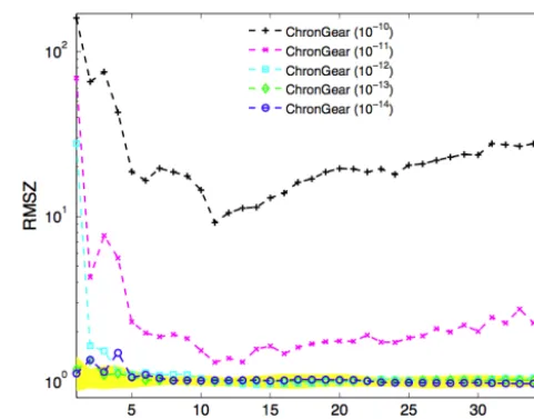
Figure 2.Monthly root mean squareZ-score (RMSZ) of temper-ature with respect to an ensemble (denoted by yellow) for experi-ments with barotropic different convergence tolerances. Note that this is subset of Fig. 13 in Hu et al. (2015).
(a precursor to the CESM-ECT approach) for CESM-POP data. In particular, Hu et al. (2015) created an ensemble con-sisting of 40 runs of 36 months in length that differed by an O(10−14)perturbation in the initial ocean temperature field. Next, the root mean squareZ-score between the new case,
e
X, and the ensemble of test cases was calculated as follows. If size of ensembleEis denoted byNens, then at each grid pointi,Nens values exist for each variableX. The average and standard deviation at each grid pointi for theNens en-semble members ofEare denoted byµiandσi, respectively.
Recalling thatnis the number of grid points, for each vari-ableXein the new run, the root mean squareZ-score ofXeas
compared to ensembleEis
RMSZ(X, E)e = v u u t
1 n
n
X
i=1
(exi−µi
σi
)2. (1)
Figure 2 shows the results of the root mean squareZ-scores (RMSZs) for the same five selected convergence tolerances as in Fig. 1, and now the error induced by the least strict toler-ances is more evident. Based on this result in Fig. 2, Hu et al. (2015) evaluated the suitability of a new solver in CESM-POP.
2.3 Ensemble consistency testing for the Community Atmosphere Model
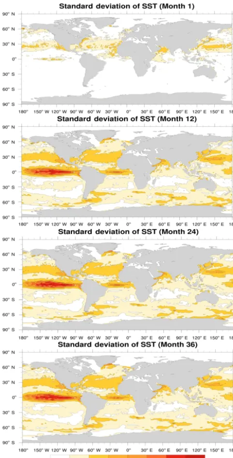
dis-Figure 3.The ensemble distribution for the standard deviation of sea surface temperature (SST) at months 1, 12, 24, and 36.
tinguishable from the ensemble of runs, then the new run is deemed “consistent”. Statistical consistency is a key ingredi-ent in the quality assurance aspect of model code verification (Oberkamf and Roy, 2010). The CESM-ECT approach was first applied to history output from the CAM component, re-sulting in the CAM-ECT tool. CAM data were a logical first target as the timescales for changes to propagate throughout the atmosphere are shorter compared to other CESM com-ponents and CAM contains a large number of independent variables that cover the whole globe.
As described in Baker et al. (2015), the ensemble for CAM-ECT is created on a trusted machine with an accepted version and configuration of CESM. The ensemble consists of 151 simulations of 1 year in length that differ only in a ran-dom perturbation of the initial atmospheric temperature field ofO(10−14). The output data contain only the annual aver-ages at each grid point for the number of specified variables from CAM, denoted byNvar, which represent whole atmo-spheric fields (by default,Nvar=120). The CAM-ECT tool creates a statistical distribution that characterizes the ensem-ble using principal component analysis (PCA) on the global area-weighted mean distributions for each variable across the ensemble. The distribution of principal component (PC) scores are retained for comparison with new simulation runs. A small set of new runs (generally three) either passes or fails based on the number of PC scores that fall outside a specified confidence interval (typically 95 %). Parameters specifying the pass/fail criteria can be tuned to achieve a desired false positive rate for the test.
2.4 Motivation
3 A new statistical consistency test for POP
Expanding the CESM-ECT suite to include a consistency test for CESM-POP data, which we denote POP-ECT, re-quires determining an appropriate ensemble to represent ocean model variability and developing a methodology to ad-dress ocean-specific characteristics. We first discuss the en-semble creation. We then describe the new testing procedure.
3.1 POP ensemble construction
We evaluate whether differences in CESM-POP output data are statistically significant (i.e., indicative of a changed cli-mate state) by comparing to an ensemble of simulations rep-resenting an accepted ocean state. Therefore, the first stage in applying the CESM-ECT approach to CESM-POP data is creating an appropriate ensemble. Clearly, the ensemble composition is critical to an effective test, and simulations should be produced on an accepted machine with an accepted version of CESM. Note that as compared to CAM, the ocean model has fewer independent diagnostic variables: tempera-ture (TEMP), SSH, salinity (SALT), and the zonal and merid-ional velocities with respect to the model grid (UVEL and VVEL, respectively). Of these five variables, SSH is 2-D and the remainder are 3-D.
For POP-ECT, we create an ensemble EofNens simula-tions, denoted by E= {E1, E2, . . ., ENens}, that differ only
by an O(10−14) perturbation to the initial ocean tempera-ture field. This initial perturbation size is on the order of double-precision round-off error and should not be climate-changing. The size of the ensemble must be sufficient to create a representative distribution, but as small as possi-ble to avoid high computational cost. While we address in detail our choice of ensemble size later in Sect. 5, we use Nens = 40 for the discussion in this section and the experi-ments in the next. Our experiexperi-ments indicate that this choice of ensemble size adequately represents the natural variability in the ocean for testing purposes. The ensemble simulation data consist of monthly temporal averages at each grid point ifor the five POP diagnostic variables: TEMP, SSH, SALT, UVEL, and VVEL. Each of these variable data setsX con-tainsNXgrid points and is denoted byX= {x1, x2, . . ., xNX},
wherexi is a scalar monthly average at grid pointi. Data are
collected forT months (i.e.,T time slices of monthly data). The next step in CESM-ECT approach is to characterize the ensemble distribution in a qualitative way to facilitate the evaluation of new runs. This statistical description of the en-semble is stored in a so-called enen-semble summary file and is associated with the CESM software tag used to generate the ensemble simulations. The history files from theNens simu-lations do not need to be retained once the summary file has been created. Recall that for CAM data, CAM-ECT calcu-lates the global-weighted-area mean for each variable from the annual temporal averages available at each grid point. This calculation results in a distribution ofNensglobal means
for each variable. However, this approach of using global-weighted-area means will not be appropriate for ocean model data, as ocean variability is less heterogeneous across the grid than atmospheric data.
For example, consider an ensemble ofNens = 40 CESM simulations with a 1◦ resolution CESM-POP grid run for T = 36 months. In Fig. 3, we show spatial panels of the standard deviations of the sea surface temperature (SST), across the ensemble members after 1, 12, 24, and 36 months. Note that the SST is simply the top layer of the 3-D vari-able TEMP (more precisely, the top 10 m of upper ocean). Figure 3 shows that the standard deviation is far from hetero-geneous with orders of magnitude differences across the grid (see the color bar scale). Also notable is the change from 1 to 12 months associated with the model instability associated with the development of hydrodynamic instability of the flow as the model spins-up. At the end of 1 year, the larger stan-dard deviation in the tropical regions suggest a larger uncer-tainty due to the growth of tropical instability waves (Leg-eckis, 1977) in the ensembles. The large variability can be easily enhanced in the equatorial regions because of the finer resolution in the tropics (approximately 1/3◦). There are also some pools of large standard deviation in the downstream of the major ocean current systems. The change from 12 months to 36 is more subtle, indicating the associated physical in-stability may not grow further due to the ocean dissipation. Given the range in variability evident in Fig. 3, the RMSZ score strategy as used for verification in Hu et al. (2015) (and discussed in Sect. 2) may include the uncertainty introduced by the actual physical instability in regions with large vari-ability (e.g., the equatorial Pacific) and may unnecessarily flag potential errors in regions with little to no variability due to the denominator in Eq. (1). Note the range of vari-ability shown in Fig. 3 is certainly resolution dependent, and the results in Fig. 3 are specific to the rather dissipative low-resolution ocean model (e.g., 1◦CESM-POP) used in most climate studies.
Therefore, to create an ensemble statistical consistency test that is robust for CESM-POP data, we must create a dis-tribution describing the ensemble that contains spatial as well as temporal information. In particular, POP-ECT creates an ensemble file withT monthly time slices of CESM-POP data that contains
– Nvar×NX×T monthly mean values across the ensemble
at each grid pointi(µi)
– Nvar×NX×T standard deviations of ensemble monthly
mean values at each grid pointi(σi),
which is to say that we retain the ensemble mean and stan-dard deviation at each ofNx grid points (note that NX
de-pends on whetherXis a 2-D or 3-D variable) for the speci-fied number of months, e.g.,T = 36.
in the closed marginal seas because there is no apprecia-ble freshwater feedback between the freshwater and salin-ity (e.g., Hudson Bay, the Mediterranean Sea). The current CESM-POP has strong freshwater restoring in the marginal seas, and weak restoring elsewhere, a salinity restoring to the Polar Science Center Hydrographic Climatology version 2 (updated from Steele et al., 2001). These specific treatments can maintain a salinity balance but act as artificial forcings to the model dynamics. Therefore, in this work we do not address the complexity of how to do verification properly in the marginal seas and instead restrict our attention to the open oceans.
3.2 Testing procedure
Given the POP-ECT summary file, we determine whether new simulation output data (e.g., from a code modification, a new machine, a new compiler option) are statistically con-sistent with the ocean climate categorized by the reference ensemble distribution as follows. We take the approach of evaluating the standardized difference between the ensemble and the new runat each grid point. For each grid pointiand each new variable X, we calculate the distance betweene Xe
and the ensemble data via a standardZ-score measurement for a given monthly time slicet. In particular, given the val-ues ofXeat timet,Xe= {ex1,t,ex2,t, . . .,exNX,t}, theZ-score at
grid pointifor variableXeat timetis
Zexi,t=
exi,t−µi,t
σi,t
,
whereµi,tandσi,tare the ensemble mean and standard
devi-ation, respectively, at grid pointifor variableXat the speci-fied monthtas specified in the ensemble summary file.
Now for a particular time slicet, we drop all subscriptst from relevant variables, e.g., the Z-score becomesZ
e xi. We
define an allowable tolerance tolZ for the Z-score at each
point, meaning that ifZxei>tolZ, then pointi is denoted a
“failed” point. Recall that a Z-score indicates the number of standard deviations away from the mean, and a large Z-score indicates that the new case is far from its climate state in the ensemble. Next we look at the overall percentage of grid points that have passingZscores, defining theZ-score passing rate (ZPR) for variableXeas
ZPR e X=
no.{i|
e
xi∈Xe ∧ |Z
e
xi| ≤ tolZ}
no.{i|
e
xi∈Xe}
. (2)
To make an overall determination of whether variableXe
passed, we set a minimum threshold for the ZPR (minZPR). In particular, if ZPR
e
X≥minZPRthen variableXepasses. By
default, the Z-score tolerance is tolZ = 3.0, and the ZPR
threshold is minZPR = 0.9. In other words, 90 % of the new values for variableXemust be within 3.0 standard deviations
of the ensemble mean (µi) at each grid point i for Xe to
“pass”. This process is repeated for all five independent
di-agnostic variables, and all variables must pass for the overall simulation to be deemed statistically consistent.
Note that the calculatedZscores change with simulation length. Because of the longer timescales present in the ocean, we ran the CESM simulations for most of the experiments in the paper for 36 months. In addition, we output monthly time slice data for POP-ECT (as opposed to the annual tem-poral mean for CAM-ECT) to determine whether the ensem-ble ocean states stabilize (or not) over time. In addition, for some of the experimental results in this paper, we find it more useful to plot theZ-score failure rate (i.e., 1−ZPR) than the ZPR.
As will be evident in the following section, the ZPRs gen-erally become stable after a few months, and the stability trends across the diagnostic variables are similar. Therefore, in addition to picking a suitableZ-score tolerance and pass-ing rate, we choose a checkpoint (tC) at which to evaluate the new run result (instead of checking at allT months of data). Note that the length of the ensemble simulations does not need to be longer thantC.
3.3 Software tools
given for each ocean model variable at the selected check-point timetC.
4 Experiments
The primary objective of this section is to evaluate the new POP-ECT tool on CESM-POP simulation data with a series of experiments on configurations with expected outcomes, including revisiting the effect of changing the barotropic solver convergence tolerance as in Hu et al. (2015) and dis-cussed in Sect. 2. Experiments were run with the CESM 1.2.2 release with the default Intel 13.2.1 compiler, using CESM-POP for the active ocean component, the CICE (Commu-nity Ice Code) model for the active sea ice component, and data-driven atmosphere and land components. In addi-tion, we use the climatologically averaged atmospheric forc-ing (1-year repeatforc-ing forcforc-ing) framework for ocean-ice sim-ulations. Therefore, there are no year-to-year correspond-ing events (such as El Niño–Southern Oscillation, ENSO), and the variance in the equatorial Pacific may be artifi-cially suppressed. (Note that this particular CESM compo-nent configuration is referred to in CESM documentation as a “G_NORMAL_YEAR” component set.) The CESM grid resolution was “T62_g16”, which corresponds to a 1◦ grid (320×384) for the ocean and ice components, with 60 verti-cal levels and a displaced Greenland pole. Simulations were run on 96 processor cores on the Yellowstone machine at NCAR (unless otherwise specified).
For these experiments, we evaluate 36 months of data as opposed to a single time slice to provide insight as to how the ZPRs vary over time and guide the selection oftC. Fur-ther, to illuminate the relationship between theZ-score and simulation month in terms of ZPR and guide the selection of tolZand minZPR, we utilize a response surface methodol-ogy (RSM) (e.g., Box and Draper, 2007). That is, we provide plots of the response surfaces for variableXewhere the
per-centage of grid pointsithat meet theZ-score tolerance cri-teria, Z
e
xi>tolZ, are shown with a cumulative distribution
function (CDF) for a range of tolZ values and simulation
months. Finally, as noted previously, we find an ensemble size of 40 to be sufficient for our experiments, but we further explore and discuss the ensemble size parameter selection in Sect. 5.
For simplicity, we show results for TEMP and SSH. Though we analyzed the other variables as well, these two are representative of the ocean system model in general as SSH is related to ocean circulation dynamics and TEMP is determined by model scalar transport.
4.1 Barotropic solver convergence tolerance
First we use the newly enhanced CESM-ECT to revisit the ef-fect of changing the barotropic solver convergence tolerance, as discussed in Sect. 2 in reference to the work in Hu et al.
(2015). The default barotropic solver convergence tolerance in CESM-POP is 10−13, and we ran experiments with con-vergence tolerances ranging from 10−9to 10−16, outputting monthly temporal averages at each grid point for 36 months. We expect convergence tolerances tighter than the default 10−13 to result in a consistent climate, but looser tolerances to introduce some error.
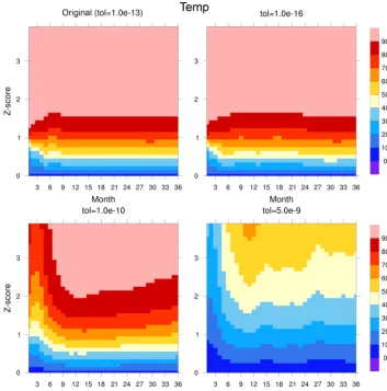
Response surfaces for TEMP and SSH are given in Figs. 4 and 5, respectively. Each figure contains four response sur-faces: the original default convergence tolerance (10−13) and a tighter tolerance (10−16) in the top two panels and looser tolerances (10−10and 5.0×10⁻⁹) in the bottom two panels. For each response surface, thex axis indicates the simula-tion month (ranging from 1 to 36), and they axis indicates the range ofZ-score values used for tolZ when calculating
the percentage of grid points that fall below theZ-score tol-erance, i.e., ZPR in Eq. (2) . The color bar indicates the ZPR as a percentage in increments of 10 %. The response surface panels are useful for evaluating various combinations of op-tions for tolZ and minZPR. For example, consider the effect on variable TEMP of modifying the solver convergence toler-ance. The upper left panel in Fig. 4 indicates that for the orig-inal convergence tolerance (10−13), 90 % of all grid points had aZ-score of less than 2.0 at all simulation months. In contrast, the panel below for 10−10shows that after the first 9 simulation months, 90 % of the grid points have aZ-score less 3.0, and by 12 months, between 70 and 80 percent of the grid points have Z-scores less than 2.0. Further loosening the convergence tolerance to 5.0×10⁻⁹as in the lower right panel shows pronounced errors in terms of the relatively low ZPR percentages. If we turn our attention to SSH in Fig. 5 for the same four convergence tolerances, the overall trends are similar. In particular, for 10−13, 90 % of all grid points have aZ-score of less than 2.0 at all simulation months (except month 6). Similarly to TEMP, the panel for 10−10shows that errors have been introduced and errors are even more pro-nounced for 5.0×10⁻⁹. A notable difference between the response surfaces for TEMP and SSH is that the panel for temperature are smoother over time because diffusion is an important process in the temperature calculation.
If we fix theZ-score tolerance for the data shown in Figs. 4 and 5, we can more easily evaluate the ZPR (consider setting tolZ = 3.0, a rather conservative choice). Figure 6
illus-trates the percentage of grid points withZ-scores that exceed tolZ = 3.0 (i.e.,fail) for both TEMP and SSH. If we choose
ex-Figure 4.Response surfaces forZ-score of temperature (TEMP) over time (monthly) andZ-score tolerance. Each panel represents a different barotropic solver convergence tolerance (labeled above). The color bar indicates the percentage of grid points with aZ-score below theZ -score tolerance (on theyaxis).
ceeding theZ-score tolerance increases. This result is much clearer than in Hu et al. (2015).
4.2 Processor layouts
While CESM simulations that are identical except for differ-ing numbers of CESM-POP processor cores yield non-BFB identical results, the results from such simulations should represent the same climate state (i.e., they should not be sta-tistically distinguishable). Here we verify that such tions definitively pass CESM-ECT. Recall that the simula-tions comprising our CESM-ECT ensemble were run on 96 cores. We ran additional simulations on 48, 192, and 384 cores. Note that we are not using threading in CESM-POP at this time.
The response surface panels for 96 cores (labeled “origi-nal”) and 384 cores are the top panels in Figs. 8 and 9 for TEMP and SSH, respectively. These panels show that for both core counts, 90 % of all grid points have aZ-score of less than 2.0 for nearly all simulation months, and as
ex-pected, there is little discernable difference between the two core counts for both variables. As before, we fix theZ-score tolerance at tolZ = 3.0 and show the Z-score failure rates
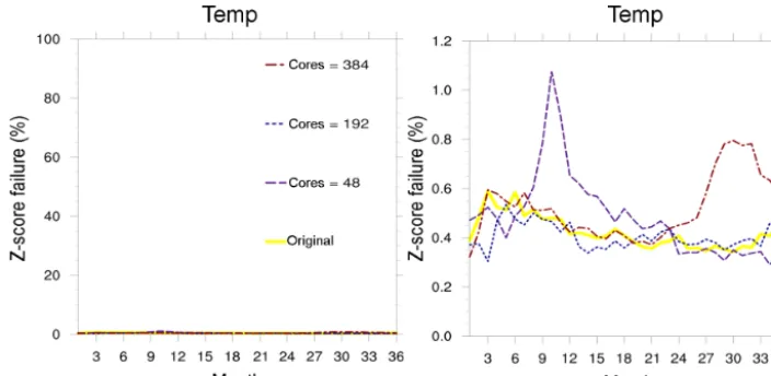
for TEMP with all four core count options (48, 96, 192, and 384) in Fig. 7. As anticipated, theZ-score failure percent-ages are quite low (below 1.2 %) for all configurations at all monthly time slices, confirming that differences in simula-tion output due to varying the core count in CESM-POP are not statistically significant and correctly identified as such by the new CESM-ECT methodology. Note that the correspond-ing panel for SSH is not provided as is looks similarly good in terms of very lowZ-score failure rates.
4.3 Physical parameters
Figure 5.Response surface forZ-score of sea surface height (SSH) over time (monthly) andZ-score tolerance. Each panel represents a different barotropic solver convergence tolerance (labeled above). The color bar indicates the percentage of grid points with aZ-score below theZ-score tolerance (on theyaxis).
Figure 7.Percentage of grid points withZ-scores for temperature (TEMP) that exceed the 3.0 tolerance for simulations with various numbers of processor cores. (Note that the left and right panels contain the same information, with different scales for theyaxis.)
coefficient for convective instability (convect_diff) is set to beconvect_diff= 10 000 for the tracer mixing coefficient in the 1◦CESM-POP configuration. We increase this parameter by factors of 2, 5, and 10, which is expected to increase the vertical mixing in the ocean interior when the density pro-file is unstable. This should noticeably impact the CESM-POP results due to the different mixing property. Second, we change the POP tracer advection scheme (t_advect_ctype) from the default third-order upwind scheme (upwind3) to the Lax–Wendroff scheme with 1-D flux limiters (lw_lim). This change is also significant and should lead to a different cli-mate state because the associated diffusion and dispersion errors differ.
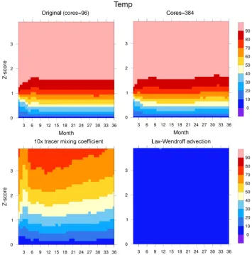
The response surface panels for increasingconvect_diffby a factor of 10 are given in the lower left panels in Figs. 8 and 9 for TEMP and SSH, respectively. This change clearly af-fects the climate state significantly, particularly as compared to changing the CESM-POP core count to 384 as depicted in the upper right panel in both figures. In fact, the impact on TEMP of increasing convect_diff in Fig. 8 is almost as strong as changing the solver convergence tolerance to 10−9 in Fig. 4. The change of the advection scheme also leads to different climate state, evident in the lower right panels in Figs. 8 and 9 for TEMP and SSH, respectively. Note that the Z-scores at nearly every grid point are failing.
The Z-score failure rates for tolZ = 3.0 are shown in
Fig. 10 for advection scheme change as well as all the modifi-cations to the tracer vertical mixing coefficient for convective instability. If we choose a ZPR threshold of minZPR = 0.9, which corresponds to a maximum of 10 % Z-score fail-ure rate, then doubling the vertical mixing coefficient ( con-vect_diff×2) is borderline in terms of passing or failing. The remaining tests clearly fail for both TEMP and SSH, as expected. Based on our experiments thus far, choosing aZ-score tolerance of tolZ = 3.0 and a ZPR threshold of
minZPR = 0.9 yields the expected outcome, and these pa-rameter settings are the default for the pyCECT tool.
4.4 Simulation length
Our experiments in Fig. 10 indicate that the percentage of grid points with failingZ-scores differs little from month to month after the first 12 months for both TEMP and SSH. This conclusion can also be reached from Figs. 8 and 9 for TEMP and SSH, respectively. In particular, the response of SSH to the initial temperature perturbation is largely stabi-lized after 12 months. The SSH may be affected through the circulation change resulting from the change of density strat-ification. Based on our experimental results, evaluating the output at a single well-chosen checkpoint time tC appears reasonable.
ad-Figure 8.Response surfaces forZ-score of temperature (TEMP) over time (monthly) andZ-score threshold. The top two panels represent two different processor core layouts. The bottom left has a tracer mixing coefficient for convective instability that is 10 times larger than the original (100 000.0), and the bottom right uses a different tracer advection scheme (Lax–Wendroff scheme with 1-D flux limiters). The color bar indicates the percentage of grid points with aZ-score below theZ-score tolerance (on theyaxis).
vection scheme significantly changes the numerical dissipa-tion and diffusion associated with the scheme (Tseng, 2008) and effectively influences the circulation pattern and struc-ture in the ocean model (e.g., Tseng and Dietrich, 2006). In particular, the Lax–Wendroff scheme with flux limiters can introduce excessive numerical mixing, which may interact with the physical mixing of temperature and salinity, though it can result in a much smoother solution in general.
4.5 Hardware and compiler modifications
A primary quality assurance responsibility of POP-ECT is to ensure that changes to either the hardware or software stack do not negatively affect POP-CESM simulation output. Here we use POP-ECT to evaluate the consistency of simula-tions that result for compiler or hardware modificasimula-tions that lead to non-BFB results, but are not expected to be climate-changing. We run POP-ECT with the default parameters
sug-gested in the previous subsections:tC = 12, tolZ = 3.0,
En-Figure 9. Response surfaces forZ-score of sea surface height (SSH) over time (monthly) and Z-score threshold. The top two panels represent two different processor core layouts. The bottom left has a tracer mixing coefficient for convective instability 10 times larger than the original (100 000.0), and the bottom right uses a different tracer advection scheme (Lax–Wendroff scheme with 1-D flux limiters). The color bar indicates the percentage of grid points with aZ-score below theZ-score tolerance (on theyaxis).
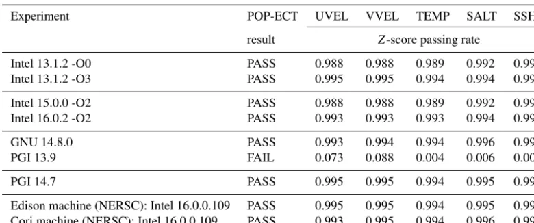
Table 1.Z-score passing rate (ZPR) for POP-ECT with default parameterstC = 12, tolZ = 3.0, and minZPR = 0.9 for each of the five diagnostic variables (described in Sect. 3.1). Note that the top seven experiments all use NCAR’s Yellowstone machine.
Experiment POP-ECT UVEL VVEL TEMP SALT SSH
result Z-score passing rate
Intel 13.1.2 -O0 PASS 0.988 0.988 0.989 0.992 0.992 Intel 13.1.2 -O3 PASS 0.995 0.995 0.994 0.994 0.996
Intel 15.0.0 -O2 PASS 0.988 0.988 0.989 0.992 0.992 Intel 16.0.2 -O2 PASS 0.993 0.993 0.993 0.994 0.995
GNU 14.8.0 PASS 0.993 0.994 0.994 0.996 0.992 PGI 13.9 FAIL 0.073 0.088 0.004 0.006 0.002
PGI 14.7 PASS 0.995 0.995 0.994 0.995 0.996
Edison machine (NERSC): Intel 16.0.0.109 PASS 0.995 0.995 0.994 0.995 0.996 Cori machine (NERSC): Intel 16.0.0.109 PASS 0.993 0.995 0.994 0.996 0.997
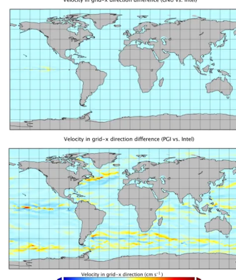
ergy Research Scientific Computing Center (NERSC). Ta-ble 1 indicates that all of these simulations resultspassthe POP-ECT, with the exception of thefailresult for PGI 13.9 on Yellowstone. The failure for PGI 13.9 suggests that some aspect of the CESM-POP code may be sensitive to this com-piler version. While we have not determined why PGI 13.9 causes the discrepancy in simulation output, POP-ECT ap-propriately returns a failas notable differences do exist be-tween the default Intel 13.1.2 and the PGI 13.9 simulations (as compared, for example to differences between the default Intel 13.1.2 and GNU 14.8 simulations), as shown for the top-level zonal velocity (UVEL) in Fig. 12. Note, however, that results with PGI 14.7 are consistent, perhaps indicating a correction in this more recent version of PGI.
5 Ensemble size
The size (i.e., number of members) of the ensemble must be large enough to sufficiently capture ocean model variability, but as small as possible for computational efficiency. In this section, we discuss the sensitivity of POP-ECT to ensem-ble size. We setup experiments to determine the false posi-tive rate associated with multiple ensembles sizes as follows. First, we generate a total of 80 ensemble members that differ by anO(10−14)perturbation to the initial ocean temperature field. Second, from the 80 members, we remove 10 to use as our test set. Next, from the remaining 70 members, we create ensembles of sizes 10, 20, 30, 40, 50, and 60. In par-ticular, for each ensemble size, we do 100 random draws for each ensemble size from the set of 70 members, resulting in 100 distinct ensembles corresponding to each ensemble size. Then for each ensemble size, we run POP-ECT at tc=12
months for each of the 10 members of the test set with all 100 ensembles of that size, resulting in 1000 tests per ensem-ble size. We consider the measured experimental failure rate to be the type I error, or “false positive” rate. Since the test
set and the ensemble members are all drawn from the larger 80 member collection that represents a statistically consistent climate, theZ-score failure rate would ideally be as low as possible.
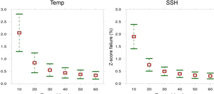
Figure 13 shows the results of performing these experi-ments for variables TEMP and SSH. Thexaxis indicates the ensemble size, and they axis indicates theZ-score failure rate. For each ensemble size, the squares denote the mean and the error bars indicate 1 standard deviation of uncertainty. As expected, as the ensemble size increases, the false positive rate decreases and the range of uncertainty shrinks. How-ever, increasing the ensemble size has diminishing returns; the improvement in false positive rate when using 20 instead of 10 members is much greater than the improvement gained by using 60 instead of 50 members. We choose an ensemble size of 40 as improvement beyond that is marginal and we balance a low false positive rate with keeping the cost of the ensemble generation low.
6 Additional discussion: scope and limitations
Figure 11.Z-score of sea surface temperature (SST) at month 12 for the original (default) case, a 384 processor core case, a case with a 10 times larger tracer mixing coefficient for convective instability (100 000.0), and a case with an alternate tracer advection scheme (Lax–Wendroff scheme with 1-D flux limiters).
bases (Kay et al., 2015). In fact, because our purpose here and in Baker et al. (2015) is not to evaluate the climate con-sistency in the coupled climate production simulation but to identify potential errors induced during the software develop-ment life cycle, our design for POP-ECT minimizes the natu-ral variability introduced by the surface boundary conditions and other potential forcing by using the climatological data-driven forcing. ENSO or low-frequency variability
simula-Figure 12.Differences in the top-level zonal velocity (UVEL) in cm s−1at month 12. The top panel shows the differences between the GNU 14.8 and default Intel simulation output. The lower panel shows the differences between PGI 13.9 and the default Intel 13.1.2 simulation outputs. Note that the min, max, and mean data values for UVEL for the default Intel 13.1.2 simulations at month 12 (top-level) are−80.9, 77.0, and−0.8 cm s−1, respectively. For compari-son, the min, max, and mean data values for UVEL are−87.9, 69.8, and−0.9 cm s−1for the PGI 13.9 simulation data.
tions will fail the POP-ECT if coupled simulations are con-ducted because of the chaotic behaviors in the atmosphere model.
Figure 13.The distributions of experimental failure rates based on 1000 tests for the variables temperature (TEMP) and sea surface height (SSH). For each ensemble size, the green bars indicate the maximum and minimum values obtained, and the red boxes indicate the mean.
7 Conclusions and future work
Since the CESM-POP ocean model is widely used and crit-ical to many climate simulations, assuring its quality is of paramount importance. However, the chaotic nature of ocean dynamics often leads to simulation results that are not identi-cal in the presence of minor differences, such as a change in processor core count for the simulation. Therefore, the ability to easily determine whether differences in model re-sults are statistically significant is important to both climate scientists and model developers. The ensemble methodology developed for evaluating consistency with atmospheric data, CAM-ECT, was not appropriate for ocean simulation data based on its differing characteristics. Therefore, we devel-oped a new ocean model-specific methodology for statistical consistency testing, POP-ECT, that allows for the subjective detection of statistically significant changes in CESM-POP. Together with the new methodology, using an appropriately sized ensemble is critical as well. Our experiments indicate the appropriateness of the new approach for detecting differ-ences in the model ocean state. The addition of POP-ECT to the CESM-ECT suite of tools has greatly enhanced the capa-bility to ensure quality CESM simulations in the midst of the ongoing state of CESM development and continually evolv-ing hardware and software environments.
We plan to extend this work in a number of ways. First, the existing spatial approach lends itself to the examination of re-gional ocean diagnostics. For example, named oceans could be identified individually as the source of failure if the global test fails. Enabling the move from coarse- to fine-grain diag-nostics would facilitate determining the root cause of an er-ror or difference. Second, we plan to extend the evaluation of the effects of data compression on climate data in Baker et al. (2014) to ocean model data and will use the testing method-ology presented here to evaluate the impact. The ability to determine whether changes in the ocean state are statistically significant or not due to data loss during compression is
crit-ical to the acceptance of compression as a tool to reduce data volumes for ocean simulation data.
8 Code availability
The CESM-ECT Python tools (pyCECT v2.0) can be obtained independently of CESM from NCAR’s public git repository (https://github.com/NCAR/PyCECT/releases). The version of CESM used for our experiments, CESM 1.2.2, is available at http://www.cesm.ucar.edu/models/cesm1.2. The CESM-ECT software tools are also included in the CESM public releases, with the POP-ECT addition available starting with the CESM 2.0 release series. CESM-POP simu-lation data are available from the corresponding author upon request.
Acknowledgements. This research used computing resources
provided by the Climate Simulation Laboratory at NCAR’s Com-putational and Information Systems Laboratory (CISL), sponsored by the National Science Foundation and other agencies. This research used resources of the National Energy Research Scientific Computing Center, a DOE Office of Science User Facility sup-ported by the Office of Science of the U.S. Department of Energy under contract no. DE-AC02-05CH11231. This work is supported in part by a grant from the National Natural Science Foundation of China (41375102) and the National Grand Fundamental Research 973 Program of China (no. 2014CB347800).
References
Baker, A. H., Xu, H., Dennis, J. M., Levy, M. N., Nychka, D., Mick-elson, S. A., Edwards, J., Vertenstein, M., and Wegener, A.: A Methodology for Evaluating the Impact of Data Compression on Climate Simulation Data, in: Proceedings of the 23rd Interna-tional Symposium on High-performance Parallel and Distributed Computing, HPDC ’14, 203–214, 2014.
Baker, A. H., Hammerling, D. M., Levy, M. N., Xu, H., Dennis, J. M., Eaton, B. E., Edwards, J., Hannay, C., Mickelson, S. A., Neale, R. B., Nychka, D., Shollenberger, J., Tribbia, J., Verten-stein, M., and Williamson, D.: A new ensemble-based consis-tency test for the Community Earth System Model (pyCECT v1.0), Geosci. Model Dev., 8, 2829–2840, doi:10.5194/gmd-8-2829-2015, 2015.
Box, G. E. P. and Draper, N. R.: Response Surfaces, Mixtures, and Ridge Analyses, Second Edition, John Wiley and Sons, 2007. Carson, II, J. S.: Model Verification and Validation, in: Proceedings
of the 2002 Winter Simulation Conference, 52–58, 2002. Clune, T. and Rood, R.: Software Testing and Verification
in Climate Model Development, IEEE Software, 28, 49–55, doi:10.1109/MS.2011.117, 2011.
Easterbrook, S. M., Edwards, P. N., Balaji, V., and Budich, R.: Guest Editors’ Introduction: Climate Change – Science and Software, IEEE Software, 28, 32–35, 2011.
Hu, Y., Huang, X., Baker, A. H., Tseng, Y., Bryan, F. O., Den-nis, J. M., and Yang, G.: Improving the scalability of the ocean barotropic solver in the Community Earth System Model, in: Proceedings of the International Conference for High Perfor-mance Computing, Networking, Storage and Analysis, SC ’15, 42:1–42:12, doi:10.1145/2807591.2807596, 2015.
Hurrell, J. W., Holland, M. M., Gent, P. R., Ghan, S., Kay, J. E., Kushner, P. J., Lamarque, J. F., Large, W. G., Lawrence, D., Lindsay, K., Lipscomb, W. H., Long, M. C., Mahowald, N., Marsh, D. R., Neale, R. B., Rasch, P., Vavrus, S., Vertenstein, M., Bader, D., Collins, W. D., Hack, J. J., Kiehl, J., and Mar-shall, S.: The Community Earth System Model: A Framework for Collaborative Research, B. Am. Meteorol. Soc., 94, 1339– 1360, doi:10.1175/BAMS-D-12-00121.1, 2013.
Kay, J., Deser, C., Phillips, A., Mai, A., Hannay, C., Strand, G., Ar-blaster, J., Bates, S., Danabasoglu, G., Edwards, J., Holland, M., Kushner, P., Lamarque, J.-F., Lawrence, D., Lindsay, K., Mid-dleton, A., Munoz, E., Neale, R., Oleson, K., Polvani, L., and Vertenstein, M.: The Community Earth System Model (CESM) Large Ensemble Project: A Community Resource for Studying Climate Change in the Presence of Internal Climate Variability, B. Am. Meteorol. Soc., 96, 1333–1349, 2015.
Legeckis, R.: Long waves in the eastern equatorial Pacific: A view from geostationary satellite, Science, 196, 1177–1181, 1977. Oberkamf, W. and Roy, C.: Verification and Validation in Scientific
Computing, Cambridge University Press, 13-51, 2010.
Pipitone, J. and Easterbrook, S.: Assessing climate model software quality: a defect density analysis of three models, Geosci. Model Dev., 5, 1009–1022, doi:10.5194/gmd-5-1009-2012, 2012. Smith, R., Jones, P., Briegleb, B., Bryan, F., Danabasoglu, G.,
Den-nis, J., Dukowicz, J., Fox-Kemper, C. E. B., Gent, P., Hecht, M., Jayne, S., Jochum, M., Large, W., Lindsay, K., Maltrud, M., Nor-ton, N., Peacock, S., Vertenstein, M., and Yeager, S.: The Parallel Ocean Program (POP) Reference Manual Ocean Component of the Community Climate System Model (CCSM), 2010. Steele, M., Morley, R., and Ermold, W.: PHC: A global ocean
hydrography with a high-quality Arctic Ocean, J. Climate, 14, 2079–2087, 2001.
Stocker, T., Qin, D., Plattner, G., Tignor, M., Allen, S., Boschung, J., Nauels, A., Xia, Y., Bex, B., and Midgley, B.: IPCC, 2013: Climate Change 2013: the physical science basis, Contribution of working group I to the fifth assessment report of the Intergov-ernmental Panel on Climate Change, 2013.
Tseng, Y.-H.: High-order essentially local extremum diminishing schemes for environmental flows, Int. J. Numer. Meth. Fl., 58, 213–235, doi:10.1002/fld.1725, 2008.