www.geosci-model-dev.net/9/4521/2016/ doi:10.5194/gmd-9-4521-2016
© Author(s) 2016. CC Attribution 3.0 License.
Ice Sheet Model Intercomparison Project (ISMIP6)
contribution to CMIP6
Sophie M. J. Nowicki1, Anthony Payne2, Eric Larour3, Helene Seroussi3, Heiko Goelzer4,5, William Lipscomb6, Jonathan Gregory7,8, Ayako Abe-Ouchi9,10, and Andrew Shepherd11
1NASA Goddard Space Flight Center, Greenbelt, MD 20771, USA
2School of Geographical Sciences, University of Bristol, Bristol, BS8 1SS, UK
3Jet Propulsion Laboratory, California Institute of Technology, Pasadena, CA 91109, USA
4Institute for Marine and Atmospheric Research, Utrecht University, Utrecht, 3584 CC, the Netherlands
5Laboratoire de Glaciologie, Université Libre de Bruxelles, CP160/03, Av. F. Roosevelt 50, 1050 Brussels, Belgium 6Los Alamos National Laboratory, Los Alamos, NM 87544, USA
7Department of Meteorology, University of Reading, Reading, RG6 6BB, UK 8Met Office Hadley Center, Exeter, EX1 3BP, UK
9Atmosphere and Ocean Research Institute, The University of Tokyo, Kashiwa-shi, Chiba 277-8564, Japan 10Japan Agency for Marine-Earth Science and Technology, Yokohama, Japan
11School of Earth and Environment, University of Leeds, Leeds, LS2 9JT, UK
Correspondence to:Sophie M. J. Nowicki ([email protected])
Received: 29 April 2016 – Published in Geosci. Model Dev. Discuss.: 26 May 2016
Revised: 30 September 2016 – Accepted: 2 December 2016 – Published: 21 December 2016
Abstract.Reducing the uncertainty in the past, present, and future contribution of ice sheets to sea-level change requires a coordinated effort between the climate and glaciology com-munities. The Ice Sheet Model Intercomparison Project for CMIP6 (ISMIP6) is the primary activity within the Coupled Model Intercomparison Project – phase 6 (CMIP6) focusing on the Greenland and Antarctic ice sheets. In this paper, we describe the framework for ISMIP6 and its relationship with other activities within CMIP6. The ISMIP6 experimental de-sign relies on CMIP6 climate models and includes, for the first time within CMIP, coupled ice-sheet–climate models as well as standalone ice-sheet models. To facilitate analysis of the multi-model ensemble and to generate a set of standard climate inputs for standalone ice-sheet models, ISMIP6 de-fines a protocol for all variables related to ice sheets. ISMIP6 will provide a basis for investigating the feedbacks, impacts, and sea-level changes associated with dynamic ice sheets and for quantifying the uncertainty in ice-sheet-sourced global sea-level change.
1 Introduction
Ice sheets constitute the largest and most uncertain potential source of future sea-level rise (Church et al., 2013; Kopp et al., 2014). The Greenland and Antarctic ice sheets currently hold ice equivalents of over 7 and 57 m of sea-level rise, respectively. Observations indicate that the Greenland and Antarctic ice sheets have contributed approximately 7.5 and 4 mm of sea-level rise over the 1992–2011 period (Shepherd et al., 2012) and that their contribution to sea-level rise is ac-celerating (Rignot et al., 2011a). Sea-level change has been identified as a long-lasting consequence of anthropogenic cli-mate change, as sea levels will continue to rise even if tem-peratures are stabilized (Meehl et al., 2012). Therefore, as-sessing whether the observed rate of mass loss from the ice sheets will continue at the same pace, or accelerate, is crucial for risk assessment and adaptation efforts.
oceanic circulation (e.g., Weaver et al., 2003) and marine bio-geochemistry (Raiswell et al., 2006). Changes in ice-sheet orography modify near-surface temperatures by altering at-mospheric circulation (Ridley et al., 2005) on both regional and global scales (e.g., Manabe and Broccoli, 1985). Surface albedo and elevation change due to the waxing and waning of ice sheets has played an important role in past interglacial– glacial transitions (e.g., Calov et al., 2009; Abe-Ouchi et al., 2013). Seasonal fluctuations in ice-sheet albedo can also exert considerable influence on local surface energy fluxes (e.g., Box et al., 2012), through both melt and snowfall. Over longer timescales, changes in ice-sheet elevation can cause a positive feedback on surface mass balance, wherein a thin-ning ice sheet experiences warmer temperatures at lower ele-vations, which causes further melting and thinning. Ice-sheet elevation changes can also alter the local climate, for instance changing the trajectory of Southern Ocean storms that pene-trate onto the Antarctic Plateau (Morse et al., 1998).
Ice sheets gain mass primarily by accumulation of snow-fall, and lose mass through a combination of surface melt-water runoff, surface sublimation, iceberg discharge to the ocean, and basal melting (under both grounded ice and float-ing ice shelves). The Antarctic Ice Sheet experiences min-imal surface melt and thus loses mass primarily through basal melting and iceberg calving. Most basal mass loss in Antarctica occurs under ice shelves (e.g., Joughin and Pad-man, 2003; Pritchard et al., 2012), but sub-ice-sheet meltwa-ter is also produced over large areas (Fricker et al., 2007). Together, basal melting and iceberg calving currently out-weigh snowfall accumulation to the Antarctic Ice Sheet (Rig-not et al., 2013; Depoorter et al., 2013). The Greenland Ice Sheet is also currently losing mass overall; this occurs pri-marily through iceberg calving and surface runoff. Surface mass balance changes have recently surpassed iceberg calv-ing changes as the dominant contributor to Greenland mass loss (van den Broeke et al., 2009), with increased surface runoff now contributing 60 % of the mass loss (Enderlin et al., 2014). Due to the long response time of ice sheets, mass changes observed at present are a complex combination of the response to present climate changes as well as past cli-mate changes as far back as several tens of thousands of years. These integrating effects of ice sheets and the vastly different timescales on which ice-sheet models and climate models operate have historically inhibited efforts to interface these two components of the Earth system.
Previously, ice sheets were not explicitly included in the CMIP process, and separate modeling studies were used to make projections of their future contributions to sea level. This has often led to mismatches between the climate data used to force these models and the contemporary version of the CMIP projections. This mismatch was perhaps accept-able when ice sheets were regarded as passive elements of the climate system on sub-millennial timescales (e.g., Church and Gregory, 2001). Observations of rapid mass loss as-sociated with dynamic change in the ice sheets, however,
have highlighted the need to couple ice sheets to the rest of the climate system. At one stage, this mismatch was such that little confidence could be placed in the projections of ice-sheet models, which were felt to omit the key pro-cesses responsible for observed changes (e.g., Meehl et al., 2007). With subsequent developments in ice-sheet model-ing, many of the processes thought to affect ice-sheet dy-namics on sub-centennial timescales (such as grounding-line migration, changes in basal lubrication, and, to some ex-tent, iceberg calving) can be simulated with some confidence (e.g., Church et al., 2013). Previous ice-sheet model inter-comparison exercises have played a crucial role in this de-velopment. An excellent example is the ongoing series of inter-comparisons aimed at understanding issues associated with the numerical modeling of grounding-line motion (e.g., Pattyn et al., 2012, 2013). Two previous international efforts, the SeaRISE and ice2sea initiatives, supplied projections on which the assessments of Church et al. (2013) were based. A major criticism of both efforts, however, was that they were based on forcing from the Special Report on Emissions Sce-narios (SRES, Naki´cenovi´c et al., 2000) rather than the cur-rent Representative Concentration Pathway (RCP, van Vu-uren et al., 2011) framework. The Ice Sheet Model Intercom-parison Project for CMIP6 (ISMIP6) is explicitly designed to ensure that ice-sheet (hence sea-level) projections are fully compatible with the CMIP6 process.
ISMIP6 brings together for the first time a consortium of international ice-sheet models and coupled ice-sheet–climate models. This effort will thoroughly explore the sea-level con-tribution from the Greenland and Antarctic ice sheets in a changing climate and assess the impact of large ice sheets on the climate system. In this paper, we provide an overview of the ISMIP6 effort and present the ISMIP6 framework. We begin by explaining the objectives and approach for ISMIP6 (Sect. 2), and describe the experimental design (Sect. 3). We next present an evaluation and analysis plan (Sect. 4) and fi-nally discuss the expected outcome and impact of ISMIP6 (Sect. 5).
2 Objectives and approach
con-tribute to answering the question “How can we assess future climate change given climate variability, climate predictabil-ity, and uncertainty in climate scenarios?” for scenarios in-volving the mass budget of the ice sheets and its impact on global sea level.
ISMIP6 targets two Grand Science Challenges (GCs) of the WRCP: “Melting Ice and Global Consequences” and “Regional Sea-level Change and Coastal Impacts”. Specifi-cally, the primary goal of the ISMIP6 effort is to improve our understanding of the evolution of the Greenland and Antarc-tic ice sheets under a changing climate. A related goal is to quantify past and future sea-level contributions from ice sheets, including the associated uncertainties. These uncer-tainties arise from unceruncer-tainties in both the climate input and the response of the ice sheets. A secondary goal is to investi-gate the role of feedbacks between ice sheets and climate in order to gain insight into how changes in the ice sheets will affect the Earth climate system.
These goals require an experimental framework that can address the following objectives.
– Develop better models of climate and ice sheets, as both coupled systems and individual components.
– Improve understanding of how ice sheets respond to cli-mate on various timescales, both in the past and in the future.
– Improve understanding of how ice sheets affect local and global climate, and explore ice-sheet–climate feed-backs.
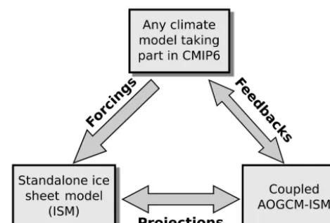
– Improve simulation of sea-level change, especially pro-jections for the 21st century and over the next 300 years. As depicted in Fig. 1, our goals and objectives rely on three distinct modeling efforts: (i) traditional CMIP atmosphere– ocean general circulation models (AOGCM/AGCMs) with-out dynamic ice sheets, (ii) standalone dynamic ice-sheet models (ISMs) that are driven by provided forcing fields (“offline”), and (iii) atmosphere–ocean climate models cou-pled to dynamic ice sheets (AOGCM–ISMs), which, as de-scribed in the following sections, can be combined to form an integrated framework.
3 ISMIP6 experimental design
Following the CMIP6 protocol, the ISMIP6 experiments both use and augment the CMIP6-DECK (Diagnostic Eval-uation and Characterization of Klima) and Historical sim-ulations (Meehl et al., 2014; Eyring et al., 2016). In addi-tion, ISMIP6 collaborates with the CMIP6-Endorsed Paleo-climate Model Intercomparison effort (PMIP4, Kageyama et al., 2016) and builds on the CMIP6-Endorsed ScenarioMIP (O’Neill et al., 2016) that focuses on future climate experi-ments for CMIP6. For a selected number of AGCM/AOGCM
Figure 1.Overview of the ISMIP6 effort designed to obtain forcing from climate models, project sea-level contributions using ice-sheet models, and explore ice-sheet–climate feedbacks.
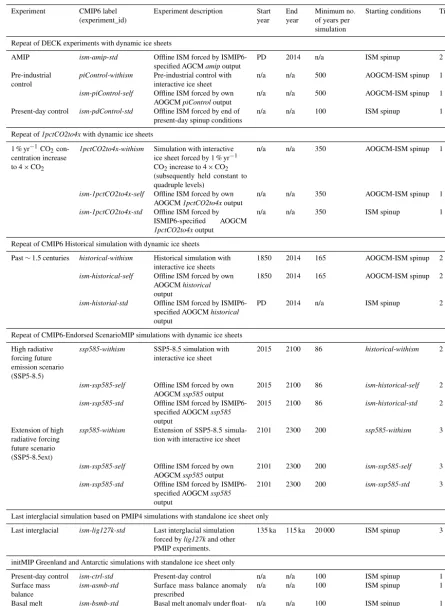
experiments that are already part of CMIP6 (Table 1 and de-scribed in Sect. 3.1), three additional model configurations are proposed, “XXX-withism”, “ism-XXX-self”, and “ ism-XXX-std”, whereXXXstands for different forcing scenarios as described later and shown in Table 2. The first case, “ XXX-withism”, indicates that the ice-sheet model is run interac-tively with the climate model (the AOGCM–ISM configu-ration described in Sect. 3.2). The other two cases describe an offline, or “standalone”, ice-sheet model that is driven by outputs from either an uncoupled AOGCM “ism-XXX-self” (the ISM configuration described in Sect. 3.2) or from a stan-dard ISMIP6 dataset “ism-XXX-std” that will be provided for the glaciology community (the ISM configuration described in Sect. 3.3). The goal of theism-XXX-selfsimulations is to obtain an ice-sheet evolution and sea-level contribution that can be compared to the AOGCM-only and AOGCM-ISM ex-periments in order to gain insight into the feedbacks between ice sheets and climate. Differences between theism-XXX-self
runs and AOGCM–ISM runs will be attributable to ice-sheet feedbacks on other climate components. The ism-XXX-std
experiments will complement the AOGCM and AOGCM– ISM experiments by using ice-sheet configurations and forc-ing datasets that are as realistic as possible, aimforc-ing to min-imize the effects of AOGCM biases. Theism-XXX-std sim-ulations target mainly the glaciology community and aim to simulate realistic ice-sheet evolution for sea-level estimates. A related set of standalone experiments, called initMIP, will explore uncertainties associated with the initialization of ice-sheet models for Greenland and Antarctica.
3.1 Analysis of experiments with climate models proposed elsewhere in CMIP6 (and not coupled to ISMs)
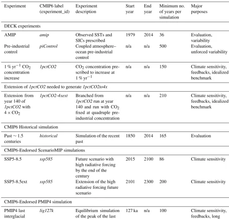
Table 1.Overview of the experiments with climate models not coupled with ice-sheet models that are to be used by ISMIP6. All experiments are started on 1 January and end on 31 December of the specified years. n/a stands for not applicable.
Experiment CMIP6 label Experiment Start End Minimum no. Major
(experiment_id) description year year of years per purposes
simulation
DECK experiments
AMIP amip Observed SSTs and
SICs prescribed
1979 2014 36 Evaluation,
variability Pre-industrial
control
piControl Coupled atmosphere– ocean pre-industrial control
n/a n/a 500 Evaluation,
unforced variability
1 % yr−1CO2 concentration increase
1pctCO2 CO2concentration pre-scribed to increase at 1 % yr−1
n/a n/a 150 Climate sensitivity,
feedbacks, idealized benchmark
Extension of1pctCO2needed to generate1pctCO2to4x
Extension from year 140 of
1pctCO2with 4×CO2
1pctCO2-4xext Branched from
1pctCO2run at year 140 and run with CO2 fixed at quadruple pre-industrial concentration
n/a n/a 210 Climate sensitivity,
feedbacks, idealized benchmark
CMIP6 Historical simulation
Past∼1.5 centuries
historical Simulation of the recent past
1850 2014 165 Evaluation
CMIP6-Endorsed ScenarioMIP simulations
SSP5-8.5 ssp585 Future scenario with
high radiative forcing by the end of the century
2015 2100 86 Climate sensitivity
SSP5-8.5ext ssp585 Extension of the high
radiative forcing future scenario
2101 2300 200 Climate sensitivity
CMIP6-Endorsed PMIP4 simulation
PMIP4 last interglacial
lig127k Equilibrium simulation of the peak of the last interglacial period
127 ka n/a 100 Climate sensitivity,
feedbacks, long responses
and coupled atmosphere–ocean general circulation models (AOGCMs) over and surrounding the polar ice sheets. This part of ISMIP6 can be viewed as diagnostic in the sense that all climate models that participate in CMIP6 will be included in this assessment without requiring extra work from the cli-mate modeling centers. These experiments do not include dynamic ice sheets, and as explained in the CMIP6 proto-col (Eyring et al., 2016), climate modeling centers that con-tribute to CMIP6 are required to submit simulations for the DECK and CMIP6 Historical runs. Our goals are to establish the suitability of the CMIP models for producing climate in-put for ice-sheet models and to assess the uncertainty in pro-jections of sea-level change arising from such climate input.
As described in Sect. 4, an additional goal is to assess past and projected changes in surface forcing (here for a fixed ice-sheet extent and topography), along with the resulting sea-level contribution from both ice sheets due to changes in sur-face freshwater flux alone. The largest uncertainty in century-scale sea-level projections, however, remains the dynamic ice-sheet response to changes in atmospheric and oceanic conditions, which will be addressed by the other components of ISMIP6 (Sect. 3.2 and 3.3).
Table 2. Overview of the ISMIP6 experiments with dynamic ice sheets that are either coupled to climate models (AOGCM-ISM, XXX-withism) or run offline (ISM,ism-XXX-self, andism-XXX-std). All experiments are started on 1 January and end on 31 December of the specified years. PD indicates that the start date corresponds to the date of the present-day ISM spinup. n/a stands for not applicable.
Experiment CMIP6 label Experiment description Start End Minimum no. Starting conditions Tier (experiment_id) year year of years per
simulation Repeat of DECK experiments with dynamic ice sheets
AMIP ism-amip-std Offline ISM forced by ISMIP6-specified AGCMamipoutput
PD 2014 n/a ISM spinup 2 Pre-industrial
control
piControl-withism Pre-industrial control with interactive ice sheet
n/a n/a 500 AOGCM-ISM spinup 1
ism-piControl-self Offline ISM forced by own AOGCMpiControloutput
n/a n/a 500 AOGCM-ISM spinup 1 Present-day control ism-pdControl-std Offline ISM forced by end of
present-day spinup conditions
n/a n/a 100 ISM spinup 1 Repeat of1pctCO2to4xwith dynamic ice sheets
1 % yr−1CO 2
con-centration increase to 4×CO2
1pctCO2to4x-withism Simulation with interactive ice sheet forced by 1 % yr−1 CO2increase to 4×CO2
(subsequently held constant to quadruple levels)
n/a n/a 350 AOGCM-ISM spinup 1
ism-1pctCO2to4x-self Offline ISM forced by own AOGCM1pctCO2to4xoutput
n/a n/a 350 AOGCM-ISM spinup 1
ism-1pctCO2to4x-std Offline ISM forced by ISMIP6-specified AOGCM
1pctCO2to4xoutput
n/a n/a 350 ISM spinup 1
Repeat of CMIP6 Historical simulation with dynamic ice sheets Past∼1.5 centuries historical-withism Historical simulation with
interactive ice sheets
1850 2014 165 AOGCM-ISM spinup 2
ism-historical-self Offline ISM forced by own AOGCMhistorical
output
1850 2014 165 AOGCM-ISM spinup 2
ism-historial-std Offline ISM forced by ISMIP6-specified AOGCMhistorical
output
PD 2014 n/a ISM spinup 2
Repeat of CMIP6-Endorsed ScenarioMIP simulations with dynamic ice sheets High radiative
forcing future emission scenario (SSP5-8.5)
ssp585-withism SSP5-8.5 simulation with interactive ice sheet
2015 2100 86 historical-withism 2
ism-ssp585-self Offline ISM forced by own AOGCMssp585output
2015 2100 86 ism-historical-self 2
ism-ssp585-std Offline ISM forced by ISMIP6-specified AOGCMssp585
output
2015 2100 86 ism-historical-std 2
Extension of high radiative forcing future scenario (SSP5-8.5ext)
ssp585-withism Extension of SSP5-8.5 simula-tion with interactive ice sheet
2101 2300 200 ssp585-withism 3
ism-ssp585-self Offline ISM forced by own AOGCMssp585output
2101 2300 200 ism-ssp585-self 3
ism-ssp585-std Offline ISM forced by ISMIP6-specified AOGCMssp585
output
2101 2300 200 ism-ssp585-std 3
Last interglacial simulation based on PMIP4 simulations with standalone ice sheet only Last interglacial ism-lig127k-std Last interglacial simulation
forced bylig127kand other PMIP experiments.
135 ka 115 ka 20 000 ISM spinup 3
initMIP Greenland and Antarctic simulations with standalone ice sheet only
Present-day control ism-ctrl-std Present-day control n/a n/a 100 ISM spinup 1 Surface mass
balance
ism-asmb-std Surface mass balance anomaly prescribed
n/a n/a 100 ISM spinup 1 Basal melt ism-bsmb-std Basal melt anomaly under
float-ing ice prescribed (Antarctica only)
experimental protocol is available elsewhere in this special issue. ISMIP6 uses three of the four DECK experiments de-scribed in Eyring et al. (2016). The Atmospheric Model In-tercomparison Project (amip, Gates et al., 1999) simulation allows the evaluation of the atmospheric component of cli-mate models given prescribed sea surface temperatures and sea ice conditions. These oceanic forcings are based on ob-servations and range from January 1979 to December 2014 for CMIP6 (see Appendix A1.1 of Eyring et al., 2016). The pre-industrial control, piControl, is a coupled atmospheric and oceanic simulation with constant conditions, chosen to represent pre-industrial values (with 1850 as the reference year; see Appendix A1.2 of Eyring et al., 2016).piControl
serves as the starting point for many simulations and is meant to capture the pre-industrial quasi-equilibrium state of the climate system. It allows an evaluation of model drift and provides insight into the unforced internal variability. The DECK also contains two idealized “climate change” exper-iments, in which the CO2 concentration is varied to gain insight into the Earth system response to basic greenhouse gas forcing. ISMIP6 will focus on a 1pctCO2to4x simula-tion, a slightly modified version of the DECK1pctCO2 sim-ulation. The1pctCO2simulation is 150 years long, starting from thepiControl, with a 1 % yr−1increase in atmospheric CO2 concentration. The 1pctCO2to4xsimulation is identi-cal to 1pctCO2 for the first 140 years, at which point the CO2concentration reaches 4 times the initial value. At this point, 1pctCO2to4xbranches from1pctCO2 and continues with constant quadrupled CO2. (Note that the1pctCO2to4x scenario was called1pctCO2in CMIP5 (Taylor et al., 2012) and1pctto4xin CMIP3.) In order to produce boundary condi-tions for theirism-1pctCO2to4x-selfsimulation, groups par-ticipating in ISMIP6 with a coupled AOGCM–ISM should carry out a1pctCO2-4xextsimulation, which starts from year 140 of their 1pctCO2 simulation and runs for a minimum of 210 years (and ideally 360 years; see Sect 3.2) with CO2 concentration held fixed. The1pctCO2to4xfields will not be stored in the CMIP6 archive, but can be generated by merg-ing the outputs from the first 140 years of the1pctCO2run with that from1pctCO2-4xext.
The CMIP6 Historical simulation,historical, tests the ca-pability of AOGCMs to simulate the historical period, de-fined as 1850 to 2014. The forcing is derived from observa-tions of solar variability and changes in atmospheric com-position, including both anthropogenic and volcanic sources (see Appendix A2 of Eyring et al., 2016). The more dis-tant past is the focus of PMIP4, which designs paleocli-mate experiments (Kageyama et al., 2016; Otto-Bliesner et al., 2016). ISMIP6 collaborates with PMIP4 for experi-mentlig127k, a simulated time slice of the Last Interglacial (LIG): the warm period from 129 000 to 116 000 years ago when global mean sea level was 5–10 m higher than present (Masson-Delmott et al., 2013). The future in CMIP6 falls un-der the guidance of ScenarioMIP (O’Neill et al., 2016); IS-MIP6 will focus on the high-emission scenario ssp585that
produces a radiative forcing of 8.5 W m−2in 2100 and its ex-tension to 2300, to evaluate climate and ice-sheet changes in response to a large forcing. If time permits, lower-emission mitigation scenarios will also be included in the ISMIP6 standalone ice-sheet framework.
Evaluation of the climate over and surrounding the ice sheets is necessary both to establish the suitability of current climate models to provide forcing for ice-sheet models and to gain insight into sea-level uncertainty arising from uncer-tainty in atmospheric and oceanic climate forcings. Of partic-ular interest is the surface climate over the ice sheets, with a focus on temperature and surface mass balance (SMB). SMB is defined as total precipitation minus evaporation, sublima-tion, and surface runoff, where runoff is meltwater less any refreezing within the snowpack. Because the ocean condition is prescribed for theamipsimulation but not for the histori-calsimulation, we expect that the temperature and SMB pro-vided by the two simulations over the same time period will differ. We will explore our second interest, the capability of climate models to reproduce the oceanic state in the vicinity of the ice sheets, using thehistoricalsimulation.
The general approach for evaluating the atmospheric com-ponent of climate models over the ice sheets (e.g., Yoshimori and Abe-Ouchi, 2012; Fettweis et al., 2013; Vizcaíno et al., 2013; Cullather et al., 2014; Lenaerts et al., 2016) is to com-pare the large-scale atmospheric state over the polar regions, the local climate, and processes at the ice-sheet surface. The latter focuses on whether the climate model can simulate snow processes, including albedo evolution and refreezing, at a horizontal resolution that captures the SMB gradients at ice-sheet margins. Both the atmospheric components and factors that can affect atmospheric processes are often eval-uated. One example is determining whether sea ice condi-tions are adequately captured inhistoricalsimulations (e.g., Lenaerts et al., 2016), as sea ice can influence moisture avail-ability and therefore precipitation. However, adequate mod-eling of precipitation also requires well-resolved ice-sheet topography (orographic forcing), which remains challenging for coarse-resolution climate models (Vizcaíno, 2014).
on the ice-sheet surface. Such stations include, for example, the 15 Greenland stations known as the GC–Net (Steffen and Box, 2001), the Greenland PROMICE network with a focus on the ablation zone (Ahlstrøm et al., 2008), and, in Antarc-tica, the Neumayer Base (Lenaerts et al., 2010). These sta-tions also record winds and temperatures. The surface tem-perature over the ice sheets may also be evaluated from satel-lite observations, using, for example, data derived from the Moderate Resolution Imaging Spectroradiometer (MODIS, Hall et al., 2012). These remotely sensed temperature prod-ucts show the onset and/or spatial extent of surface melt (e.g., Mote et al., 1993; Hall et al., 2013), which can then be used to assess whether the climate models capture the relevant processes at the ice-sheet surface (e.g., Fettweis et al., 2011; Cullather et al., 2016). However, a full understanding of why surface melt varies from model to model may require investi-gations that include cloud properties (Van Tricht et al., 2016). The current generation of climate models participating in CMIP6 is unlikely to simulate ocean circulation in ice-shelf cavities or within fjords. Thus, evaluation of the ocean state around the ice sheets involves first establishing that the cli-mate models can reproduce certain properties of the key wa-ter masses. Ocean circulation around the Greenland Ice Sheet involves a complex interaction between polar waters of Arc-tic origin and AtlanArc-tic waters from the subtropical North At-lantic (Straneo et al., 2012). The mechanisms that transport warm water through fjords and toward the ice fronts remain an active area of research (Wilson and Straneo, 2015; Stra-neo and Cenedese, 2015). In the Southern Ocean, important water masses include Antarctic Bottom Water and Antarc-tic Intermediate Waters. In the coastal regions, Circumpo-lar Deep Water, Antarctic Surface Water, and High Salin-ity Shelf Water are the primary oceanic influences on ice sheets (Bracegirdle et al., 2016). Given the difficulty many CMIP5 models had in capturing high-latitude ocean prop-erties, CMIP6 models should be evaluated using existing datasets (Bracegirdle et al., 2016). These datasets include Argo, expendable bathythermograph (XBT) and conductiv-ity/temperature/depth (CTD) vertical temperature and salin-ity profiles (e.g., Dong et al., 2008), sea ice extent products sourced from passive microwave instruments (e.g., Bjørgo et al., 1997; Cavalieri and Parkinson, 2012; Parkinson and Cav-alieri, 2012), sea surface temperature (SST) from WindSat and AMSR-E over the open ocean, satellite altimetry (Jason-1 and Jason-2) over the open ocean, and World Ocean Atlas 2009 climatological temperatures. For ocean models that in-clude ice-shelf cavities and ice–ocean interactions, sub-ice-shelf basal melting can be compared with glaciological esti-mates of ice-shelf melting around Antarctica (Rignot et al., 2013; Depoorter et al., 2013) derived from remote-sensing observations, as well as independent tracer–oceanographic estimates (Loose et al., 2009; Rodehacke et al., 2006). Just as regional atmospheric models will be key for evaluating the atmospheric component of climate models, regionally focused ocean models (e.g., Timmermann et al., 2012) and
ocean reanalysis products (e.g., Menemenlis et al., 2008) are likely to provide valuable insight for evaluating CMIP ocean models.
3.2 Experiments with climate models coupled to ISMs
The second component of ISMIP6 is a suite of experi-ments designed to assess the impacts of dynamic ice sheets on climate and to better understand feedbacks between ice sheets and climate. We also aim to obtain an ensemble of sea-level projections from fully coupled atmosphere– ocean–ice-sheet frameworks, which can later be compared to projections from standalone ice-sheet models (Sect. 3.3). The experiments should be identical to the corresponding standard CMIP AOGCM experiments except for the treat-ment of ice sheets, so that any observed feedbacks and impacts can be attributed to dynamic ice sheets and not to other sources. As indicated in Table 2, four coupled AOGCM-ISM simulations are proposed, whose experiment IDs arepiControl-withism,1pctCO2to4x-withism, historical-withism, and ssp585-withism. These simulations are com-plemented by four ISM simulations:ism-piControl-self, ism-1pctCO2to4x-self,ism-historical-self, andism-ssp585-self.
In theXXX-withismsetup, the ice-sheet model is run inter-actively with the AOGCM: the climate model sends a sur-face forcing (SMB at a minimum) to the ice-sheet model and receives changes in ice-sheet geometry. The land sur-face type and sursur-face elevation in the climate model are dy-namic, allowing, for example, a reduced albedo if the land surface changes from glaciated to unglaciated. Changes in the ice-sheet mass should also affect the ocean temperature and salinity, as freshwater fluxes (liquid and/or solid) and en-ergy fluxes are routed to the ocean. Liquid fluxes can orig-inate from surface runoff, subglacial drainage systems, or basal melting of the ice in contact with the ocean. Solid fluxes come from iceberg calving, which may be computed with calving laws whose details are left to the discretion of the modeling groups. Explicit iceberg models are not required. Similarly, ocean melting of ice shelves can be handled as de-sired, as long as the net freshwater flux and latent heat flux are routed consistently to the ocean model.
Initial conditions for both the ism-XXX-self experiments and theXXX-withismexperiments will be generated by run-ning the coupled AOGCM-ISM to a quasi-equilibrium state with pre-industrial forcing that represents the year 1850. Pindustrial AOGCM-ISM spinup is an area of active re-search (e.g., Fyke et al., 2014) that seeks to produce a con-sistent non-drifting coupled state corresponding to the pre-industrial climate, which is different from the contemporary state (Kjeldsen et al., 2015). The challenge is that ice sheets reach quasi-equilibrium on timescales of many millennia, more slowly than the oceans, which typically have been the slowest components of AOGCMs. To reach steady state, the ice-sheet model may have to be run for ∼10 000 years or longer. Since runs of this length are impractical for a complex climate model, the coupling between the ice-sheet model and the climate model will likely have to be asynchronous for at least part of the spinup. In this case, once the ice-sheet model has reached steady state, the coupled system should be run synchronously for an additional period before starting the experiments. ISMIP6 will not dictate spinup procedures for obtaining pre-industrial initial ice-sheet conditions, but the procedure should be documented.
Ideally, the ice-sheet model should be forced with the ac-tual SMB computed by the climate model, rather than an SMB corrected to match observed climatology. We accept that there may be biases in the atmospheric or land mod-els that can lead to an unrealistic SMB, which could result in a steady-state ice-sheet geometry that differs substantially from present-day observations. However, correcting for these biases can distort the feedbacks between ice sheets and cli-mate that we seek to investigate. We hope to learn from and ultimately reduce these biases, in the same way that biases elsewhere in the simulated coupled climate system are re-duced by greater understanding and improved model design. On the other hand, if the geometry of the spun-up ice sheet is greatly different from observations, then the initial ice sheet for the ism-XXX-self experiments may be far from steady state with the SMB forcing from the standard, uncoupled AOGCM. As a result, the ism-XXX-self experiment could have a large drift that obscures the climate signal. The drift will be quantified from the control experiments. In the case of a large drift, or if the spun-up ice sheet in the coupled system is deemed to be too unrealistic, an alternative spinup method would be to apply SMB anomalies from the AOGCM, super-posed on a climatology that yields more realistic equilibrium ice-sheet geometry.
The method used to downscale SMB (as well as oceanic forcing) from the coarse climate model grid to the finer ice-sheet model grid is left to the discretion of each group, but should be well documented. The data request for ISMIP6 in Appendix A asks modelers to report certain fields on both the atmospheric and ice-sheet grids to allow for an evalu-ation of the downscaling procedure. Also, ISMIP6 prefers that the surface-melt component of SMB be obtained from an energy-based method that conserves mass and energy, to
facilitate interpretation of the drivers of SMB variability and change (e.g., Vizcaíno, 2014). Highly parameterized meth-ods of computing surface melt, such as positive-degree-day (PDD) methods (e.g., Reeh, 1991; Bougamont et al., 2007), should be avoided. The choice of the ice-sheet model, its complexity in approximating ice flow, and ice-sheet-relevant boundary conditions (e.g., geothermal flux) are left to the modelers’ discretion. In all experiments, however, the ice sheets should not be forced to terminate at the present-day ice margin if the simulated SMB and/or the ice-sheet dynam-ics cause a margin advance.
Regardless of the spinup method, the first ISMIP6 exper-iment to be performed with the coupled AOGCM–ISM is the pre-industrial control,piControl-withism. This is a multi-century (500 years suggested) control run aiming to assess model drift and systematic bias and to capture unforced natural variability. The drift in the standalone ISM exper-iments ism-XXX-self will be quantified with a control run (ism-piControl-self). The core ISMIP6 prognostic climate change experiment is1pctCO2to4x-withism, which applies a 1 % yr−1increase in CO2concentrations over 140 years un-til levels are quadrupled, and then holds concentrations fixed for an additional 2 to 4 centuries. The1pctCO2to4x-withism
will be compared to the AOGCM simulation1pctCO2to4x
(the first 140 years of the DECK1pctCO2merged with the
1pctCO2-4xext) and toism-1pctCO2to4x-self(the standalone ISM forced by the AOGCM surface mass balance and tem-perature from1pctCO2to4x). The duration of these three ex-periments should be the same. It is suggested that the exper-iments be run for at least 350 years, and if possible for 500 years, because previous studies (e.g., Ridley et al., 2005; Viz-caíno et al., 2008, 2010) indicate that coupled AOGCM–ISM runs start to clearly diverge from uncoupled runs after about 250–300 years of simulation.
Another set of experiments repeats the CMIP6historical
andssp585simulations with a coupled AOGCM–ISM. The
historical-withismsimulation begins at year 1850 from the pre-industrial spinup and finishes at the end of 2014. This simulation is followed byssp585-withism, with experimen-tal settings and forcings as described in O’Neill et al. (2016). Thessp585-withismbegins in January 2015 and is initiated from the December 2014 results of the historical-withism
simulation. The ssp585-withism experiment is run for the 21st century and its extension to the end of the 23rd cen-tury. For completeness, these experiments are to be repeated with standalone ISM simulationsism-historical-selfand ism-ssp585-self. We accept that, with this protocol, the 2015 ice sheet is likely to be distinct from the observed ice sheet due to model drift from the Historical run, and that this will have implications for projected ice-sheet evolution (e.g., Stone et al., 2010).
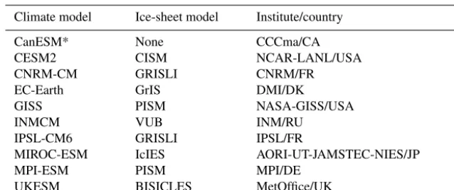
Table 3.Climate modeling centers that have expressed an interest in ISMIP6. * indicates only an interest in the diagnostic component (no AOGCM–ISM participation anticipated).
Climate model Ice-sheet model Institute/country
CanESM* CESM2 CNRM-CM EC-Earth GISS INMCM IPSL-CM6 MIROC-ESM MPI-ESM UKESM
None CISM GRISLI GrIS PISM VUB GRISLI IcIES PISM BISICLES
CCCma/CA NCAR-LANL/USA CNRM/FR DMI/DK
NASA-GISS/USA INM/RU
IPSL/FR
AORI-UT-JAMSTEC-NIES/JP MPI/DE
MetOffice/UK
ISMIP6. The primary focus is coupled ice-sheet–atmosphere simulation for the Greenland Ice Sheet, but some groups have indicated participation only in the diagnostic aspect of ISMIP6 (where the goal is to provide climate data for the standalone ice-sheet work). Full coupling of ice-sheet mod-els to climate modmod-els remains challenging, especially for in-teractions with the ocean. Accurate treatment of ice–ocean interactions requires ISMs that can simulate grounding-line migration (which demands fine grid resolution) and iceberg calving, and ocean models that can simulate circulation in the cavities below ice shelves and the consequent melting or accretion of ice on the undersides of the shelves. Accurate treatment of ice–ocean interactions will likely also require ocean models to alter their domain (both vertically and hor-izontally) as the calving front migrates and as sub-ice-shelf ocean cavities evolve in space and time. For the Greenland Ice Sheet, ocean models may need to capture fjord dynamics on smaller spatial scales (∼1 km) than are currently resolved by global ocean models. In addition, credible ice–ocean cou-pling requires accurate knowledge of the bathymetry beneath ice shelves and ice sheets, where data are sparse. Because of these challenges, we do not expect a realistic treatment of the Antarctic Ice Sheet in the ISMIP6 coupled AOGCM–ISM experiments. Antarctica is included, however, in the stan-dalone experiments described in the next section.
3.3 Experiments with ISMs not coupled to climate models
The final set of ISMIP6 experiments will use standalone ice-sheet models driven by climate model output and other datasets. Groups and models that have expressed an interest in participating in this aspect of ISMIP6 are listed in Table 4. The models participating in this effort will likely be config-ured differently from those in theism-XXX-selfsimulations described in Sect. 3.2. For example, an ice-sheet model that is spun up to quasi-equilibrium with a climate model will likely have a thickness and extent that differ appreciably from ob-served values, whereas standalone models can be initialized
more realistically. Also, an ISM in a climate model might use a coarse resolution or a simple approximation of ice dynam-ics in order to be more computationally efficient, while the same model used strictly for projections would likely have a finer resolution, at least in regions of fast flow (e.g., As-chwanden et al., 2016), and could incorporate more complex ice-flow dynamics. Similarly, ice-sheet models that are used for paleoclimate studies are often distinct from those used for projections of a few hundred years.
3.3.1 initMIP
The initMIP ice-sheet experiments are designed to explore uncertainties in sea-level projections associated with model initialization and spinup. Such uncertainties have been iden-tified by previous model intercomparison efforts (e.g., Bind-schadler et al., 2013; Nowicki et al., 2013a, b; Edwards et al., 2014a, Shannon et al., 2013; Goelzer et al., 2013; Gillet-Chaulet et al., 2012) and include the impacts of model ini-tial conditions, sub-grid-scale processes, and poorly known parameters. The initMIP project aims to evaluate initializa-tion procedures, to estimate trends caused by model initial-izations, and to investigate the impact of choices in numerical and physical parameters (e.g., stress balance approximation or model resolution). Results of the initMIP project are ex-pected to point to specific aspects of ice-sheet initialization that have a crucial impact on sea-level projections and that may be improved.
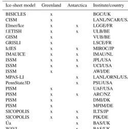
Table 4.Ice-sheet modeling groups that have expressed an interest in ISMIP6. x indicates a planned contribution.
Ice-sheet model Greenland Antarctica Institute/country
BISICLES x BGC/UK
CISM x LANL/NCAR/USA
Elmer/Ice x x LGGE/FR
f.ETISH x x ULB/BE
GISM x VUB/BE
GRISLI x LSCE/FR
IcIES x x MIROC/JP
IMAUICE x x IMAU/NL
ISSM x x JPL/USA
ISSM x x UCI/USA
ISSM x AWI/DE
MPAS-LI x LANL/ORNL/USA
PennState3D x PSU/USA
PISM x UAF/USA
PISM x x ARC/NZ
PISM x DMI/DK
PISM x MPIM/DE
SICOPOLIS x x ILTS/JP
SICOPOLIS x x PIK/DE
Úa x BAS/UK
WAVI x BAS/UK
research and a multidisciplinary effort. It requires acquisi-tion of addiacquisi-tional data with high spatial coverage over entire ice sheets and at increased resolution (e.g., Bamber et al., 2013; Rignot et al., 2011b; Joughin et al., 2010a; Howat et al., 2014). Ideally, all datasets used in the data assimilation are from the same period, as initializing an ice-sheet model with datasets taken at different times can cause the ice-flow model to artificially redistribute the glacier mass in unreal-istic ways that serve only to reconcile these inconsistencies (Seroussi et al., 2011). This also implies that the date associ-ated with the initial state can differ between models based on the datasets used. New algorithms that reconcile initializa-tion datasets are being developed, most notably for bedrock elevation (e.g., Morlighem et al., 2011, 2014), which is noto-riously poorly constrained.
The initMIP project consists of a Greenland component and an Antarctic component. Following initialization, there is a set of two forward experiments for the Greenland Ice Sheet and three forward experiments for the Antarctic Ice Sheet, each run for at least 100 years: (i) a control run ( ism-ctrl-std), (ii) a surface mass balance anomaly run (ism-asmb-std), and (iii) a basal melt anomaly run (ism-abmb-std) in which anomalous melt is applied beneath the floating portion of the Antarctic Ice Sheet. All other model parameters and forcing in the forward runs are the same as those used for initial-ization. The ism-ctrl-stdis an unforced forward experiment designed to evaluate the initialization procedure and charac-terize model drift, the surface mass balance remaining iden-tical to the one used during the initialization procedure. In
ism-asmb-std, a prescribed SMB anomaly is applied to test
the model response to a large perturbation. The schematic perturbation anomaly mimics outputs of several SMB mod-els of different complexity between the end of the 20th cen-tury and the end of the 21th cencen-tury, and is designed to cap-ture the first-order pattern of SMB changes expected from climate models. The schematic SMB anomalies are defined everywhere on the model grid, and are therefore applicable for models with varying ice-sheet extent. Inism-abmb-std, a prescribed anomaly of basal melting rate under floating ice is applied while SMB is kept the same as inism-ctrl-std. Be-cause of the difference in ice-shelf extent between the differ-ent models, the basal melt anomaly is prescribed to be con-stant for each basin. This scalar value is different for each basin and derived from the mean values of the ice-shelf melt observed by Rignot et al. (2013) and Depoorter et al. (2013). The applied anomaly simulates a doubling of sub-ice-shelf melting after 40 years of simulation for models with initial melting rates close to today’s observations.
the initMIP results to improve their initialization procedures. initMIP is also intended to give ice-sheet modelers an op-portunity to get involved in ISMIP6 at an early stage, before outputs of CMIP6 AOGCM become available; hence our pre-scription of simplified anomalies. We refer interested readers to the initMIP webpage (http://www.climate-cryosphere.org/ wiki/index.php?title=_InitMIP) for more information.
3.3.2 ism-XXX-stdconfiguration
Theism-XXX-stdexperiments target primarily the glaciology community and seek to obtain realistic ice-sheet evolution to inform estimates of past, present, and future sea levels. IS-MIP6 will supply forcing data from CIS-MIP6 that allow stan-dalone ISMs to simulate the evolution of both the Green-land and Antarctic ice sheets. ISMIP6 seeks to assess the un-certainty in sea-level change arising from both the ice-sheet models and the climate forcing. A key concern is that IS-MIP6 assess uncertainty associated with emission scenarios and the AOGCMs’ simulation of these scenarios: for a given emission scenario, the AOGCMs’ simulation of this scenario will result in a range of atmospheric and oceanic forcings. Clearly, there is a tension between the range of potential ice-sheet forcing, the need to explore uncertainty associated purely with ISMs (e.g., related to initial conditions, bedrock topography, and parametric uncertainty), and the computing requirements of specific ISMs (some of which may only be able to perform a small number of experiments). To this end, we anticipate identifying a subset of forcing from the CMIP6 AOGCM ensemble based on the analysis of AOGCM simu-lations of ice-sheet climate (Sect. 3.1). The subset will be chosen to capture the full range of potential ice-sheet forcing for a given emission scenario, using metrics of the SMB and ocean forcing to investigate that range. Within the selected subset of forcing, we plan to identify a small number of sim-ulations that all ISMs must perform. Groups that are able to perform numerous simulations will be encouraged to partic-ipate in all experiments. Shannon et al. (2013) is an example of this approach.
The forcing data can naturally be divided into atmospheric and oceanic forcing. Central to the former is the means to determine SMB associated with a particular CMIP6 exper-iment. Several methods have previously been employed to do this. Until we can assess the quality of the climate simu-lated by CMIP6 AOGCMs above and around the ice sheets (after the analysis of the CMIP6 DECK and Historical sim-ulations), a definitive choice cannot be made. However, we list the options in order of preference.
Use the SMB calculated by the AOGCM directly. This has the advantage that the SMB will be entirely consistent with other parts of that AOGCM’s simulation of climate. There is concern, however, that the quality of the SMB computed by the AOGCMs will make this approach unrealistic due primarily to the mismatch between the spatial resolution of AOGCMs and the characteristic length scale of variations in
SMB. Several groups have, however, made recent progress in this area (e.g., Vizcaíno et al., 2013; Lipscomb et al., 2013). The use of anomalies should also be considered in this con-text.
In the event that AOGCM-determined SMB is shown to be inadequate, an intermediate step is required. Previously, this has been the use of Regional Climate Models (RCMs) to sim-ulate SMB. For example, the ice2sea effort chose to generate SMB from an RCM (Edwards et al., 2014a, b; Fettweis et al., 2013). This approach, however, introduces a further link into the processing chain that may lead to delay in the produc-tion of sea-level projecproduc-tions. It also introduces the issue of choice of RCM and whether results from a number of RCMs should be used (further complicating the design of the ISM ensemble). Furthermore, the use of RCMs as intermediaries between AOGCMs and ISMs adds ambiguity about which biases are introduced by the AOGCMs and which biases are the result of the RCMs.
Use a parameterization or simplified process model to sim-ulate SMB by downscaling atmospheric forcing over the ice sheet from an AOGCM. This approach was used by SeaRISE (Bindschadler et al., 2013), where the precipitation and sur-face temperature from 18 AOGCMs models taking part in the A1B scenario were combined to generate monthly mean val-ues. These mean precipitation and temperature values were then passed to the SMB scheme of the ice-sheet model (gen-erally a PDD method that accounted for the temperature as-pect of the SMB–elevation feedback) to obtain SMB anoma-lies that were added to the ice-sheet surface conditions at ini-tialization.
A further consideration is that the AOGCM models as-sume a fixed ice-sheet elevation: i.e., they neglect the ef-fect of ice-sheet elevation change on the atmosphere and hence omit the SMB–elevation feedback. Standalone ISMs will need to include this effect by parameterizing the SMB lapse rate (Edwards et al., 2014a, b; Fettweis et al., 2013; Goelzer et al., 2013). This approach may be less of an issue for method 3 above because SMB is determined interactively within the ISM rather than being prescribed as forcing.
A second way in which the atmosphere could force dy-namic change in ice sheets is through the production of large quantities of meltwater. Mechanisms have been proposed that link meltwater to both ice-shelf collapse (Banwell et al., 2013) and enhanced lubrication of ice flow (Zwally et al., 2002) (although recent modeling studies suggest a minor in-fluence of the latter on large-scale ice flow; e.g., Shannon et al., 2013). Surface air temperature and runoff forcing will therefore also be made available.
resolution and the unique physics of ocean circulation adja-cent to melting ice. Melt rates will therefore need to be de-termined outside the climate model using an index for proxi-mal ocean temperature. This index is most likely to be water temperature (and salinity) at the continental shelf break at an intermediate range of depths (equivalent to the base of ice shelves or the depth of ice grounded on bedrock). This quan-tity will be included in our evaluation of CMIP6 forcing (see Sect. 3.1).
A wide range of approaches has been used to calculate the required melt rate from prescribed ocean-temperature forc-ing. The simplest method is to calculate melt rate anomalies from changes in the nearest ocean temperature using an ob-servationally derived relation of 10 m yr−1◦C−1(Rignot and Jacobs, 2002). However, this linear relation between ocean temperature and melt rates is calibrated for melt rates at the grounding line, and likely is missing important nonlinearities (Holland et al., 2008). An alternative approach is to param-eterize melt rates as proportional to the difference between ocean temperature at the shelf break and the freezing tem-perature at the ice-shelf base. Beckman and Goosse (2003) developed such a scheme for ocean models, and similar schemes have been applied in offline ice-sheet model simu-lations with idealized ocean forcing (e.g., Martin et al., 2011; Pollard and DeConto, 2012; DeConto and Pollard, 2016). In those studies, the ocean temperature is set to the aver-age temperature between 200 and 600 m depth (Martin et al., 2011) or the temperature at 400 m depth (DeConto and Pollard, 2016), or specified differently for specific Antarc-tic sectors (Pollard and DeConto, 2012). Depending on the evaluation of the CMIP6 models, ISMIP6 may adapt one of these choices, or could prescribe depth-varying profiles of ocean temperature (and possibly salinity). The dependence of melt rates on thermal driving ranges from linear (Martin et al., 2011) to quadratic (Pollard and DeConto, 2012; DeConto and Pollard, 2016). Since the freezing temperature at the ice base decreases with depth, the melt rates in all schemes tend to be higher near grounding lines, as found from observa-tions.
If none of the CMIP6 ocean models can accurately capture the broad-scale polar ocean circulation or produce realistic near-shelf temperatures, an alternative is to prescribe a melt rate that simply depends on the ice-shelf draft (e.g., Joughin et al., 2010b; Favier et al., 2014). This approach is less sat-isfactory, however, as it ignores temporal changes in ocean conditions, and typically uses coefficients calibrated to local thermal conditions. If ISMIP6 uses this approach, the pro-vided coefficients would not be uniform but would take into account the fact that ocean waters reaching ice-shelf cavities or fronts differ regionally. In Antarctica, for example, the ice shelves of Pine Island Glacier and Thwaites Glacier lie in “warm” water, while the Filchner-Ronne or Ross ice shelves reside in “cold” water. Ocean temperatures reflect the domi-nant water sources, with warm waters dominated by circum-polar deep waters (Jacobs et al., 2011), while cold waters
typically correspond to high-salinity shelf water (Nichols et al., 2001).
Ice–ocean interactions are an active area of research, and more sophisticated parameterizations of melt are becoming available (e.g., Jenkins, 2016; Asay-Davis et al., 2016). Sim-plified models of the system could be used (e.g., Payne et al., 2007), as could high-resolution ocean models that resolve ice-shelf cavities and fjords. Given this wide range of meth-ods, ISMIP6 will leave the detailed choice of the parameter-ization to individual ice-sheet modelers, but will issue guid-ance on what constitutes an acceptable parameterization. We will organize workshops with the polar ocean community to investigate how to best derive oceanic forcing for ice-sheet models, so that by the time the CMIP6 ocean models are evaluated, a clearer protocol will be in place. The calculated melt rate will be part of the standard data request for ice-sheet models (see Appendix A), and part of our evaluation will be to determine how well the applied forcing compares to observed melt rates of Rignot et al. (2013) and Depoorter et al. (2013).
ISMIP6 will not dictate the choice of ice-sheet model com-plexity in terms of the ice-flow approximation, the basal slid-ing law, the treatment of groundslid-ing lines, the calvslid-ing law, the ice-sheet-specific boundary conditions (e.g., bedrock to-pography), or the initialization method. An exception is that models of the Antarctic Ice Sheet should include floating ice shelves and grounding-line migration. The spatial resolution of the ISM in the vicinity of fast-flowing ice streams and the grounding line affects the dynamic response (Durand et al., 2009; Pattyn et al., 2012, 2013), and the model resolu-tion must be fine enough to capture this response accurately. To this end, participating models are encouraged to take part in model intercomparison efforts that target specific aspects of ice-sheet modeling, such as the current MISOMIP (Ma-rine Ice Sheet–Ocean Model Intercomparison Project; Asay-Davis et al., 2016), and are required to take part in initMIP (initialization-focused experiments that compare and evalu-ate the simulevalu-ated present-day stevalu-ate; Sect. 3.3.1). The lack of a stricter protocol is a reflection of the challenges in identify-ing which factors are the most important when makidentify-ing pro-jections, which datasets are most accurate, and how to best capture and parameterize certain ice-sheet processes. For ex-ample, although the choice of bedrock topography affects mass transport and is thus likely to influence a projection, it is currently not possible to identify a best dataset due to the difficulty in obtaining bedrock measurements. Groups are encouraged to repeat the experiments with a variety of per-turbations of weakly constrained parameters, boundary con-ditions, etc. in order to test the sensitivity of projections to these choices.
Unlike the protocol for climate models, theism-XXX-std
quantity of accurate, high-resolution data available during the satellite era far exceeds that available for pre-industrial and historical periods. The majority of ice-sheet models use these data in sophisticated initialization and assimilation pro-cedures, such that the present-day state of the ice sheet is simulated with high fidelity. The lack of suitable data before the satellite era means that no such accuracy can be assumed for simulations of the historical periods. Such inaccuracies are known to have a large effect on projections. For instance, discrepancies between projections can often be attributed to slight differences in the geometry (e.g., Shannon et al., 2013). The ism-XXX-stdsimulations will thus be initiated from a present-day spinup.
The firstism-XXX-stdsimulation isism-pdControl-std, the ice-sheet present-day control with constant forcing needed to evaluate model drift. This constant forcing is based on the climate at the end of the initialization procedure. For many models, the forcing and simulation will be the same as ism-ctrl-std in the initMIP experiment (Sect. 3.3.1), un-less a change has been made in the initialization. The ideal-ized climate change experiment,ism-1pctCO2to4x-std, con-siders a 1 % yr−1atmospheric CO2 concentration rise until quadrupled concentrations and stabilization thereafter. ism-historical-stdwill be an abbreviated simulation for the his-torical period (as it begins from the present-day spinup) and, following the CMIP6 protocol, ends in December 2014. ism-amip-std is a simulation for the last few decades to under-stand the well-observed record of ice-sheet changes. The re-sults fromism-amip-stdandism-historical-std are likely to differ, and the comparison will provide some insight into the relative importance of biases, climate variability, and cli-mate change. The main simulation for projecting 21st cen-tury sea-level rise isism-ssp585-std, which is initiated from theism-historical-stdsimulation. (As mentioned previously, other scenarios will be considered if time permits.) If possi-ble, projections should continue to the end of the 23rd cen-tury.
We complement the experiments for the recent past and fu-ture with one paleo experiment (ism-lig127k-std), to simulate Greenland ice-sheet evolution during the Last Interglacial. The transient simulation will span the period 135 to 115 kyr to include transitions from the preceding to following cold periods. The climate forcing forism-lig127k-stdwill be de-rived from the PMIP4-CMIP6 experimentlig127kand other (transient) LIG climate simulations (cf. Bakker et al., 2013; Lunt et al., 2013) that will be performed by PMIP4 (Otto-Bliesner et al., 2016). The proposed experiment builds on past efforts to study Greenland ice-sheet stability and evolu-tion during the LIG and constrain the Greenland contribuevolu-tion to the LIG sea-level highstand (e.g., Robinson et al., 2011; Born and Nisancioglu, 2012; Helsen et al., 2013).
3.4 Prioritization of experiments and timing
The ISMIP6 experiments listed in Table 2 are divided into three “Tiers” to indicate prioritization. Tier 1 denotes exper-iments that are to be completed by the ISMIP6 participants. Tier 2 experiments are highly encouraged, while Tier 3 ex-periments are optional.
For the coupled AOGCM–ISM experiments, the Tier 1 experiments piControl-withism and 1pctCO2to4x-withism
should be performed first. These experiments have already been performed by many climate modeling groups, and their idealized settings allow for an easier evaluation of the ice– climate feedback. The Tier 2 experiments,historical-withism
andssp585-withism, are more relevant to our goal of produc-ing sea-level projections concurrent with the CMIP6 future climate. Ideally, theXXX-withismandism-XXX-self experi-ments would follow the corresponding AOGCM experiexperi-ments with no more than a 6-month lag.
For the standalone ism-XXX-stdexperiments, ISMIP6 is constrained by the timing of the AOGCM runs that will be used to derive forcings for ice sheets. We anticipate that the DECK simulations will not be completed before the spring of 2017, which implies that climate models cannot be evalu-ated rigorously before the summer of 2017, and in turn that the ISM Tier 1 experiments based on CMIP6 DECK forc-ing would begin in 2018. As soon as suitable forcforc-ings are available from the SSP5-8.5 experiments (CMIP6-Endorsed ScenarioMIP, Tier 1),ism-ssp585-stdwill be the focus of the standalone ISM work. To allow ice-sheet modeling groups the necessary time to perform the simulations, we plan to be-ginism-ssp585-stdin early 2019. Similarly, the ism-lig127k-std cannot proceed until the PMIP participants have com-pleted the CMIP6-Endorsed PMIP4 Tier 1 experiment and other transient PMIP4 experiments. In the meantime, IS-MIP6 standalone ice-sheet models will focus on initMIP, with the goal of finishing this suite of experiments by the end of 2016 for Greenland and by the end of 2017 for Antarctica.
4 Evaluation and analysis
4.1 Evaluation of ice-sheet models
Ice-sheet models will be evaluated using methodologies al-ready in use by the ice-sheet modeling community. These metrics typically begin by assessing whether the volume and area of the modeled present-day ice sheet are comparable to observed values. The next step evaluates the spatial patterns of surface elevation, ice-sheet thickness, surface velocities, and positions of the ice front and grounding line. Some ice-sheet models are initialized using data assimilation methods, which precludes the use of certain observations in the evalua-tion. Evaluation of these models can be done by hindcasting, a method that evaluates whether recent observed trends are captured (Aschwanden et al., 2013). Examples include com-parison against the gravimetry (GRACE) time series from 2003 onwards, which provides an integrated set of measure-ments for mass changes in Greenland and Antarctica. This approach will also enable a direct comparison between pre-dicted sea-level rise from ISMs and the change in ocean mass observed by GRACE. The recent IMBIE effort (Ice Sheet Mass Balance Inter-comparison Exercise, Shepherd et al., 2012) facilitates this comparison by combining observations from gravimetry, altimetry, and velocity changes between 1992 and 2012 into a single dataset of annual mass budget for each ice sheet. The follow-on effort, IMBIE2 (A. Shep-herd, personal communication, 2015), will extend the record in time and plans to separate the observed mass change into SMB and dynamic components.
4.2 Effects of dynamic ice sheets on climate
The combination of coupled AOGCM–ISM simulations (XXX-withism) and standalone ice-sheet simulations ( ism-XXX-self) will support a clean analysis of ice-sheet feed-backs on the climate system, which can further affect ice-sheet evolution (e.g., Driesschaert et al., 2007; Goelzer et al., 2011; Vizcaíno et al., 2008, 2010, 2015). A limited number of feedbacks can be studied in an AOGCM without a dy-namic ISM. For instance, because AOGCMs generally com-pute ice-sheet SMB through a land model coupled on hourly timescales to the atmospheric model, the albedo–melt feed-back can be studied in an AOGCM alone. Other important feedbacks, however, are present only if the ice sheet is dy-namic.
As ice sheets thin, the lower elevation leads to warmer sur-face temperatures that increase melting. This ice–elevation feedback is small on sub-century timescales (Edwards et al., 2014b), but over longer timescales, it can drive ice sheets to a point of no return, where retreat would continue unabated even if the climate returned to an unperturbed state.
Changes in ice-sheet elevation modify the regional atmo-spheric circulation (e.g., Ridley et al., 2005), which can ei-ther enhance or slow the rate of retreat.
Changes in land surface cover (e.g., from glaciated to veg-etated) can darken and warm the surface, promoting atmo-spheric warming and further melting.
Increased freshwater fluxes (both solid and liquid) from retreating ice sheets can modify the density structure of the ocean, possibly suppressing convection and weakening the Atlantic meridional overturning circulation. Although some studies (e.g., Hu et al., 2009) find that this is a small effect, others suggest that increased runoff from the Greenland Ice Sheet has already reduced deep convection in the Labrador Sea (Yang et al., 2016).
The buoyancy of fresh glacial meltwater from sub-ice-shelf melting can modify the ocean circulation that drives the melting. On longer timescales, changes in the size and shape of sub-shelf cavities may also alter the circulation.
The ISMIP6 experiments will be performed on climate model runs lasting several centuries, long enough to allow a detailed analysis of at least the first four of these feedbacks. Ocean cavity feedbacks, however, may require further devel-opment of ocean models that can adjust their boundaries dy-namically as marine ice sheets advance and retreat.
4.3 Sea-level change
The SMB over the Greenland Ice Sheet is currently becoming less positive, thus resulting in an increasing contribution to sea-level rise due to increased surface runoff (van Angelen et al., 2014; Fettweis et al., 2011). This trend is expected to con-tinue (Fettweis et al., 2013; Rae et al., 2012), although there is a large spread in AOGCMs (Yoshimori and Abe-Ouchi, 2012). The picture is less clear for the Antarctic Ice Sheet, where both accumulation and surface melt are projected to increase (Lenaerts et al., 2016). The multi-model ensemble of the surface freshwater flux from AOGCM simulation will provide insight into the resulting contribution of past and fu-ture sea level due to changes in SMB alone.
The largest uncertainty in sea level, however, remains the dynamic contribution from the ice sheets. ISMIP6 targets the contribution of dynamic ice sheets to global sea level, via multi-model ensemble analysis of standalone ice-sheet models (ism-XXX-std). For a number of experiments, the multi-model ensemble from the ism-XXX-std will be con-trasted to the multi-model ensemble resulting from coupled AOGCM–ISM simulations (ism-XXX-withism). We expect the results of the standalone modeling (ism-ssp585-std) to be more robust for projections, as we anticipate that the spun-up ice sheet from the coupled historical simulation ( historical-withism) will differ substantially from present-day observa-tions, and these differences will alter the projected ice-sheet evolution (e.g., Stone et al., 2010; Shannon et al., 2013). The projections fromssp585-withismwill likely expose issues re-sulting from coupling dynamic ice-sheet models to climate models, motivating the community to begin resolving them.
climate input; hence the need to sample across scenarios and models. For example, the ongoing initMIP project will pro-vide insight into sea-level uncertainties resulting from ice-sheet model initialization. By repeating model runs with dif-ferent datasets, sliding laws, model resolutions, etc., initMIP will allow us to constrain the sea-level contribution asso-ciated with these choices. Ice-sheet evolution will also de-pend on climatic drivers. For instance, given a certain num-ber of AOGCMs that simulate present-day ice-sheet SMB reasonably well, comparing their SMB results under var-ious climate-change simulations will allow us to quantify climate-model-driven uncertainty in SMB. If relationships between large-scale climate drivers (e.g., regional tempera-ture and precipitation) and ice-sheet area-integral SMB can be established (e.g., Gregory and Huybrechts, 2006; Fet-tweis et al., 2013), this would allow estimation of SMB from AOGCM experiments for other climate scenarios. If possible, synergies with other CMIP6 efforts will allow us to further investigate the uncertainty in climate input. For example, the CMIP6-Endorsed High Resolution Model In-tercomparison Project (HighResMIP, Haarsma et al., 2016) and Coordinated Regional Climate Downscaling Experiment (CORDEX, Gutowski Jr. et al., 2016) may allow us to quan-tify the impacts of increased resolution on SMB.
5 Discussion and conclusion
ISMIP6 has an experimental protocol and a diagnostic pro-tocol. The experimental design uses and builds upon the core DECK and CMIP6 Historical simulations, along with selected CMIP6-Endorsed PMIP4 and ScenarioMIP simula-tions. The suite of ISMIP6 experiments involves three types of models: AOGCM/AGCM with no dynamic ice sheets, coupled AOGCM–ISM, and standalone ISM. The diagnostic protocol is based on ice-sheet-related model outputs, many of which are already present in the CMIP6 atmosphere and ocean diagnostics. The evaluation of the climate in the po-lar regions from AOGCM and AOGCM–ISM simulations will guide recommendations for existing and new ice-sheet– climate coupling efforts. ISMIP6 promotes the development of the ice-sheet component of climate models in an effort to bring both climate and ice-sheet models to greater maturity. ISMIP6 targets two of the WCRP Grand Science Challenges: “Melting Ice and Global Consequences” and “Regional Sea-level Change and Coastal Impacts”. Given the current rapid changes in the Greenland and Antarctic ice sheets, ice sheets can no longer be considered passive players in the climate system. Their contributions to future sea level will likely have considerable human and environmental impacts, and IS-MIP6 will facilitate research in this critical area.
ISMIP6 will coordinate simulation and analysis of ice-sheet evolution in a changing climate. Inclusion of ice-ice-sheet models is unique in CMIP history and is necessary to ad-vance understanding of the sea-level contribution from the Greenland and Antarctic ice sheets, the climate system re-sponse to ice-sheet changes, and the feedbacks between ice sheets and climate. ISMIP6 is thus an important step in clos-ing the gap between the climate and ice-sheet modelclos-ing com-munities. Our key output, the sea-level contribution from ice sheets, complements the projections of ocean thermal expan-sion that already sit within the CMIP framework. This im-provement will help sea level join the family of variables for which CMIP can provide routine IPCC-style projections. Ul-timately, the success of ISMIP6 relies on the broad partici-pation of the CMIP6 modeling centers, standalone ice-sheet modeling groups, and analysts of the atmosphere, ocean, and ice sheets.
6 Data availability
Appendix A: Variable request
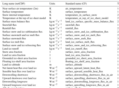
This special issue includes a manuscript that is dedicated to the CMIP6 data request. The majority of our data request is based on CMIP5 CMOR tables Amon (Monthly Mean Atmospheric Fields), Omon (Monthly Mean Ocean Fields), LImon (Monthly Mean Land Cryosphere Fields), and OI-mon (Monthly Mean Ocean Cryosphere Fields), which al-ready contained many of the outputs required to diagnose and intercompare the climate over land ice/ice sheets and to de-rive forcing for the ice sheets. In the CF convention, “land ice” comprises grounded ice sheets, floating ice shelves, glaciers, and ice caps, while “ice sheet” refers to grounded ice sheets and floating ice shelves. A few additional variables are needed to properly derive the forcings for ice sheets from AOGCMs, and to record outputs from the evolving ice sheets in the coupled AOGCM–ISM experiments (such as ice ele-vation change), or from the standalone ice-sheet simulations. In this Appendix, we briefly outline the ISMIP6 data request on the atmosphere grid (Table A1), ocean grid (Table A2), and ice-sheet grid (Table A3), and provide some context for key new variables.
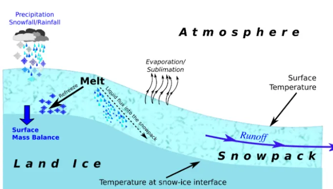
The mass change in ice sheets (see Fig. A1) is a result of the surface mass balance (SMB), ice melt (or refreeze) at the base of the grounded ice sheet (BMB), and mass exchange with the ocean. The latter can be further split into frontal mass balance (FMB, defined as iceberg calving and melt (or refreeze) at the ice-shelf front) and melt (or refreeze) at the base of ice shelves (BMB). All fluxes are defined as posi-tive when the process adds mass to the ice sheet and negaposi-tive otherwise. The thermal state of the ice-sheet models is doc-umented by the basal temperature and by the temperature at the ice-sheet–snowpack interface. Note that BMB and basal temperature are computed differently depending on whether the ice is grounded or floating, requiring the use of distinct long names but the same standard names in Table A3.