www.geosci-model-dev.net/8/2119/2015/ doi:10.5194/gmd-8-2119-2015
© Author(s) 2015. CC Attribution 3.0 License.
Evaluation of the high resolution WRF-Chem (v3.4.1) air quality
forecast and its comparison with statistical ozone predictions
R. Žabkar1,2, L. Honzak2,a, G. Skok1,2, R. Forkel3, J. Rakovec1,2, A. Ceglar4,2,b, and N. Žagar1,2 1University of Ljubljana, Faculty of Mathematics and Physics, Ljubljana, Slovenia
2Center of Excellence SPACE-SI, Ljubljana, Slovenia
3Karlsruher Institut für Technologie, Institut für Meteorologie und Klimaforschung, Atmosphärische Umweltforschung, Garmisch-Partenkirchen, Germany
4University of Ljubljana, Biotechnical Faculty, Ljubljana, Slovenia anow at: BO-MO d.o.o., Ljubljana, Slovenia
bnow at: Institute for Environment and Sustainability, Joint Research Centre, Ispra, Italy Correspondence to: R. Žabkar ([email protected])
Received: 15 January 2015 – Published in Geosci. Model Dev. Discuss.: 4 February 2015 Revised: 15 June 2015 – Accepted: 19 June 2015 – Published: 16 July 2015
Abstract. An integrated modelling system based on the re-gional online coupled meteorology–atmospheric chemistry WRF-Chem model configured with two nested domains with horizontal resolutions of 11.1 and 3.7 km has been applied for numerical weather prediction and for air quality forecasts in Slovenia. In the study, an evaluation of the air quality fore-casting system has been performed for summer 2013. In the case of ozone (O3)daily maxima, the first- and second-day model predictions have been also compared to the opera-tional statistical O3 forecast and to the persistence. Results of discrete and categorical evaluations show that the WRF-Chem-based forecasting system is able to produce reliable forecasts which, depending on monitoring site and the evalu-ation measure applied, can outperform the statistical model. For example, the correlation coefficient shows the highest skill for WRF-Chem model O3predictions, confirming the significance of the non-linear processes taken into account in an online coupled Eulerian model. For some stations and ar-eas biases were relatively high due to highly complex terrain and unresolved local meteorological and emission dynamics, which contributed to somewhat lower WRF-Chem skill ob-tained in categorical model evaluations. Applying a bias cor-rection could further improve WRF-Chem model forecasting skill in these cases.
1 Introduction
CHIMERE, Menut et al., 2013) with an output time interval typically of around 1 h. Examples are the EURAD (http://db. eurad.uni-koeln.de/index_e.html), SILAM (http://silam.fmi. fi/), ForeChem (http://atmoforum.aquila.infn.it/forechem/), CALIOPE (http://www.bsc.es/caliope/) forecast systems and others. The new generation of online coupled models (e.g. MCCM, Grell et al., 2000; GATOR-GCMM, Jacobson, 2001; Meso-NH-C, Tulet et al., 2003; WRF-Chem, Grell et al., 2005; Enviro-HIRLAM, Baklanov et al., 2008; GEM-AQ, Kaminski et al. 2008; COSMO-ART, Vogel et al., 2009; WRF-Chem-MADRID, Zhang et al., 2010a) presents an al-ternative approach with one unified modelling system, in which meteorological and air quality variables are simulated together within the same model. The online approach permits the simulation of two-way interactions between different at-mospheric processes including emissions, chemistry, clouds and radiation, and a better response of the simulated pollutant transport to changes of the wind field (Grell et al., 2004) and, thus, provides a more realistic representation of the atmo-sphere. The use of online coupled models can be particularly important in regions with high aerosol loadings and cloud coverage (Otte et al., 2005; Eder et al., 2006), where physical processes in the atmosphere may be modified by the aerosol direct effect on radiation or by aerosol–cloud interactions. Several reviews summarized the strengths and limitations of offline and online coupled models (e.g. Zhang, 2008; Klein et al., 2012; Baklanov et al., 2014). There is an increasing awareness that an integrated online approach is needed not only for assessment, forecasting and communication of air quality but also for weather forecasting (e.g. Baklanov, 2010; Grell and Baklanov, 2011; Klein et al., 2012; Zhang et al., 2012b; Baklanov et al., 2014). Nevertheless, there are sev-eral issues regarding the inclusion of chemistry into numeri-cal weather prediction models. More evidence is required to determine whether an integrated model can produce a good climatology of the most important chemical species and if such a model is, considering many uncertainties, able to beat persistence forecasts of these species (Grell and Baklanov, 2011). These questions are calling for further research and studies exploring the performance of the models with an on-line coupled chemistry.
In recent years extensive efforts have been devoted to develop air quality (AQ) forecasting systems for Slovenia. In this study we explore the use of the state-of-the-science WRF-Chem model (Grell et al., 2005) with coupled meteoro-logical, microphysical, chemical, and radiative processes for forecasting AQ in Slovenia during summertime conditions. In last decade WRF-Chem has been increasingly applied to many areas worldwide (e.g. Misenis and Zhang, 2010; Fast et al., 2009; Zhang et al., 2010a, b; Li et al., 2011; Tie et al., 2009; Hu et al., 2012; Forkel et al., 2012, Žabkar et al., 2011, 2013). In most of these studies the WRF-Chem model has been successfully used to simulate historical poor AQ conditions with a hindcast approach. To our knowledge, only a few studies focused on using WRF-Chem for
forecast-ing AQ, most of these applied the WRF-Chem forecast be-fore and during field campaigns (McKeen et al., 2005, 2007, 2009; Yang et al., 2011). Takigawa et al. (2007) evaluated the O3 forecast for a 1-month time period from a one-way nested global–regional RT-AQF system with full chemistry based on the global CHASER (Sudo et al., 2002) and re-gional WRF-Chem models, while Saide et al. (2011) eval-uated a forecast system based on the WRF-Chem model for simulating carbon monoxide (CO) as a PM10/PM2.5 surro-gate over Santiago de Chile for wintertime conditions. WRF-Chem-MADRID (Zhang et al., 2010a) with two additional gas-phase mechanisms, sectional representation for particle size distribution and more advanced model treatments com-pared to WRF-Chem, was applied by Chuang et al. (2011) and by Yahya et al. (2014) for forecasting AQ over the south-eastern US. In spite of a limited number of evaluation studies published in the literature, an increasing number of real-time weather and air quality forecasting systems based on WRF-Chem are implemented worldwide (http://ruc.noaa.gov/wrf/ WG11/Real_time_forecasts.htm).
In our study we explore the forecasting skill of WRF-Chem model over the topographically complex and geo-graphically diverse area of Slovenia for three summer months (June–August 2013). Furthermore, in the case of O3we com-pare WRF-Chem predictions with a statistical model for pre-dicting O3daily maxima, currently used at the Slovenian En-vironment Agency (SEA). Both first-day (1-day) and second-day (2-second-day) forecasts are considered, while a persistence model, which assumes that pollutant level today and tomor-row will be the same as yesterday, is used as a threshold for useful model prediction. Since the availability of an accurate and reliable forecasting system could be useful to the local authorities and could help to advise the public the proper pre-ventive actions, we want to answer the question of whether WRF-Chem model outperforms the statistical model or per-sistence. Namely, considering many uncertainties related to one unified model, it may not be easy for models with online chemistry to be able to perform well enough to meet the re-quired standards, and more research and studies are needed to investigate that (Grell and Baklanov, 2011). Due to the lim-ited number of previous studies focused on online coupled forecasting systems, the aim of our study is also to provide a greater insight into the potential that lies in the approach based on a unified model for forecasting weather and air pol-lution. Finally, identified strengths, limitations and deficien-cies of analysed RT-AQFs are expected to present the basis for further research.
2 Methodology
2.1 WRF-Chem forecast system
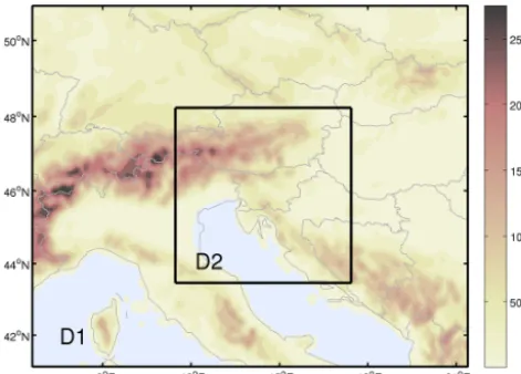
Figure 1. Modelling domains (D1, D2) used in the WRF-Chem
RT-AQF system. Orography (in metres) is shown in resolution of the D1 domain (11.1 km).
(Fig. 1) with horizontal resolutions of 11.1 and 3.7 km, and 151×100 and 181×145 grid points, respectively. A one-way nesting is applied by two separate consecutive simu-lations, where outputs from the coarse grid integration are processed to provide boundary conditions for the nested run every 15 min. The vertical structure of the atmosphere is re-solved with 42 vertical levels extending up to 50 hPa, with the highest resolution of∼25 m near the ground. About 15 lev-els are located within the lowest 2 km to assure high vertical resolution of the daytime planetary boundary layer (PBL). To produce the 48 h forecast, the model is run every day, starting at 00:00 UTC, with meteorological initial conditions (ICs) and lateral boundary conditions (BCs) taken from the 0.5◦data of the Global Forecast System (GFS) operated by the US National Weather Service (NWS). For chemical BCs, forecasts from the global MOZART-4/GEOS-5 (Emmons et al., 2010) RT-AQF system with temporal availability of 6 h are used. The instantaneous outputs at the 24th hour of the previous day’s forecast are used to initialize next day’s fore-casting simulation. An exception is the very first day of the first 48 h forecasting cycle, when global MOZART-4/GEOS-5 fields were also used to initialize chemistry. A 3-day spin-up ahead of the first analysed forecast day is then taken into account to allow pollutants to accumulate in the air masses.
In the WRF-Chem model, several choices for parame-terizations of physical and chemical processes are avail-able (Grell et al., 2005; Skamarock et al., 2008; Peckham et al., 2012) and these can have a strong impact on the model predictions. In both domains we decided to apply the same schemes as were used in simulation SI1 for phase-2 of the Air Quality Model Evaluation International Initia-tive (AQMEII) (e.g. Balzarini et al., 2015; Baró et al., 2015; Curci et al., 2015; Forkel et al., 2015; Im et al., 2015a, b; Kong et al., 2015; San Josè et al., 2015). These include the Yonsei University (YSU) PBL scheme (Hong et al., 2006),
NOAH land-surface model (Chen and Dudhia, 2001), Rapid Radiative Transfer Method for Global (RRTMG) long-wave and short-wave radiation scheme (Iacono et al., 2008), Grell 3-D ensemble cumulus parameterization scheme (Grell and Devenyi, 2002) with radiative feedback, Morrison double-moment cloud microphysics (Morrison et al., 2009), Fast-J photolysis scheme (Wild et al., 2000), RADM2 gas-phase chemistry (Regional Acid Deposition Model, Stockwell et al., 1990) and the MADE/SORGAM aerosol module (Acker-mann et al., 1995; Schell et al., 2001). Current model imple-mentation includes a modified RADM2 gas-phase chemistry solver as described in Forkel et al. (2015), which avoids un-derrepresentation of nocturnal O3titration in areas with high NO emissions. According to Forkel et al. (2015) the modi-fied solver tends to overestimate the low NO2concentration for pristine regions and in the free troposphere, which results in an overestimation of O3. Due to the focus on polluted re-gions this deficiency was considered as less important than the advantage of better description of the titration. In addi-tion, the comparatively small modelling domain (D1) ensures that the boundary conditions constrain the high bias of the modified solver for O3and NO2in the free troposphere. Also, according to our sensitivity tests (results not shown) the mod-ified solver showed better performance for O3daily maxima and O3nighttime minima than the QSSA (quasi steady state approximation) RADM2 solver supplied originally with the WRF-Chem model.
Among feedbacks only the aerosol direct effects on ra-diation according to Fast et al. (2006) and Chapman et al. (2009) are taken into account. As shown by Kong et al. (2015) for two air pollution episodes, this degree of aerosol–meteorology interactions in the 3.4.1 version of the WRF-Chem improved model performance for high aerosol loads, while the representation of the indirect effects needs to be further improved to be able to outperform simulations with direct effects only.
2.2 Statistical ozone daily maximum forecast
The statistical O3 model (Žabkar, 2011), currently used at SEA for forecasting O3 daily maxima at eight measuring sites in Slovenia (Fig. 3), is a multivariate regression tool combined with clustering algorithms to take into account measured data, weather forecast data, and the predicted back-ward trajectories of each monitoring site. As regards mea-surements, the previous day’s (at 12:00, 15:00, 18:00 and 21:00 local time, daily maximum, daily minimum, daily av-erage) and present day’s early morning (07:00 local time) meteorological (pressure, relative humidity, direct and dif-fusive solar radiation, wind speed) and AQ data (O3, NOx,
NO2, CO, PM10, SO2)are used. For meteorological predic-tions, the 24 h ECMWF forecast variables at 12:00 UTC of the forecast day at different vertical levels (1000, 925, 850, 500, 300 hPa) above the measuring sites are taken into ac-count. Among all these variables, by using the stepwise tech-nique based on F statistics, only significant variables were selected to be included in multivariate regression equations for different monitoring sites (from 15 to 26 variables, de-pending on monitoring site).
The important part of the statistical forecast is the calcu-lation of 24 h backward trajectories on meteorological fields of the ALADIN/SI forecast. The inclusion of 24 h predicted trajectories into a statistical model is based on the study of Žabkar et al. (2008) which showed that the highest O3daily maxima at monitoring sites in Slovenia are in general asso-ciated with short (slow-moving) backward trajectories with a southwestern origin, while the lowest measured daily max-imum O3 values for all the stations are associated with the clusters of long northwestern trajectories. Clusters of similar trajectories were for the purpose of the statistical forecast cal-culated byk means clustering algorithms (Moody and Gal-loway, 1988; Žabkar et al., 2008) on 6 years (2004–2010) of data (ALADIN/SI trajectories). As an example, Fig. 2 shows a mean O3daily maxima for clusters of similar trajectories for one of the monitoring sites. The same 6-year time pe-riod of training data was used in the stepwise multiple regres-sion procedure to determine the multiple regresregres-sion prognos-tic equations associated with monitoring sites and trajectory clusters, from measurements, ECMWF forecast data, average cluster O3daily maximum, and day-of-the-year variable.
The first step of the statistical O3prediction is the calcu-lation of trajectories approaching the monitoring stations at 12:00 UTC of the forecast day. In the next step, the backward trajectories of each monitoring site are associated with the nearest pre-calculated cluster of similar trajectories. Finally, the multiple regression equation of the associated group of trajectories is used to calculate the O3daily maximum pre-diction. It must also be noted that the decision on declaring O3 episodes is only partially based on the results from this statistical model, it also involves a decision made by AQ fore-casters.
Figure 2. Example of ozone analysis for the Nova Gorica (NG)
monitoring site (average daily maximum±standard deviation) for seven clusters of similar trajectories, as used in the statistical ozone daily maximum forecast for the NG station.
2.3 Evaluation methodology
signifi-Table 1. AQ monitoring sites.
Monitoring Abbreviation Type of Altitude Model Model Pollutants Statistical
site zone (m) orography analysis ozone
(m) height (m) forecast
Celje CE Urban 240 300 313 O3, PM10, NO2 No Hrastnik HRA Urban 290 540 552 O3, SO2 Yes
Iskrba ISK Rural 540 579 591 O3, NO2 Yes
Koper KOP Urban 56 72 85 O3, PM10 Yes
Kovk KOV Rural 608 516 528 NO2 No
Krvavec KRV Rural 1740 1272 1414 O3 Yes
Ljubljana LJ Urban 299 287 300 O3, PM10, NO2, Yes Murska Sobota MS Rural 188 189 202 O3, PM10, NO2 Yes Nova Gorica NG Urban 113 150 163 O3, PM10, NO2 Yes
Otlica OTL Rural 918 874 886 O3 Yes
Sv. Mohor MOH Rural 394 254 266 NO2 No
Trbovlje TRB Suburban 250 459 471 O3, PM10, NO2 No
Velenje VEL Urban 389 461 474 O3, SO2 No
Vnajnarje VNA Rural 630 468 480 NO2 No
Zadobrova ZAD Rural 280 275 287 PM10, NO2 No Zagorje ZAG Urban 241 431 443 O3, PM10, NO2 No Zavodnje ZAV Rural 765 678 690 O3, NO2 No
Figure 3. Locations of monitoring stations used in evaluation of air
quality variables (AQ stations) and meteorological variables (MET stations). Green dots indicate measuring sites with available ozone daily maximum statistical forecast (SF). For the meaning of the AQ site abbreviations see Table 1.
cantly smaller than for the first layer, while the correlation coefficient between the measured and simulated O3 levels remains similar in both cases (the fifth or the lowest model layer). Taking results from higher model layers would further decrease the negative model bias but would also worsen the correlation coefficient for O3at this station due to decreased impact of surface processes.
All AQ stations are background, seven are measuring ur-ban background, one suburur-ban and nine rural conditions. Valid O3 measurements are for the analysed time period available for 13 AQ stations. When studying the general model performance, data from four additional stations for
two other pollutants (NO2, PM10) are also analysed to get a better picture of model behaviour over the domain, known for its large topographical and climate diversity. The coverage of three climate zones in Slovenia (Mediterranean, subalpine and mountainous) with monitoring stations is the following: NG, KOP and OTL are Mediterranean sites, KRV is a moun-tainous station, and the remaining stations are subalpine. As the elevated station KRV, the ISK, OTL and VNA stations are also influenced by regional transport of pollutants.
For evaluation of predicted meteorological variables, data from SEA meteorological stations (MET, Fig. 3) for 2 m tem-perature (T2 m), 10 m wind speed (W10 m), relative humidity (RH), incoming solar radiation (SR) and precipitation (RR) are used. It must be noted that MET stations with lower spa-tial representativeness (e.g. alpine stations) were not a priori excluded from the analyses, which needs to be taken into ac-count when looking at evaluation results. The reason for not excluding these stations was that some information about the AQ forecast can also be gained by the evaluation of meteo-rological forecasts for these stations.
in-dex of agreement (IOA), the mean normalized bias error (MNBE), and the mean normalized gross error (MNGE) are calculated for O3 daily maximum concentrations predicted by the different models. Finally, to evaluate the model’s abil-ity to predict exceedances and non-exceedances, several cat-egorical indices including equitable threat score (ETS), criti-cal success index (CSI), bias (B), false alarm ratio (FAR) and probability of detection (POD) are calculated for different thresholds. Definitions of the statistical measures are shown in Appendix A.
2.4 Meteorology and air quality of June–August 2013
The analysed period was marked by three heat wave events, which contributed to the summer characterized by high tem-peratures, sunny weather and lack of precipitation in Slove-nia. The first heat wave event with a measured temperature daily maximum of up to 35◦C occurred after a rather cold beginning of the month and lasted from 15 to 21 June. The event was terminated by a cold front passage and followed by the pronounced cold episode during the end of June and the beginning of July. Another heat wave event with tempera-tures above 35◦C, observed in the lowland, started on 26 July and was briefly interrupted on 29 July, when thunderstorms related to frontal passage were accompanied by exception-ally strong wind gusts. The most remarkable of three three extraordinary hot episodes was recorded from 01 to 08 Au-gust. On the last day of this episode, 08 August, temperatures reached 40◦C at some measuring sites in Slovenia, and many of them observed their highest temperature ever recorded.
As expected for summertime conditions, measured con-centrations of most air pollutants, including PM10, were in general low during the analysed time period. The only ex-ception was O3 with exceedances of the 8 h target value (120 µg m−3)measured at all AQ monitoring stations dur-ing the three heat wave events, which is the reason why the main focus of the present study is on this pollutant. During the following two events (in July and August) threshold ex-ceedances of 1 h daily maxima were also recorded for O3. In spite of the hot and sunny conditions during the first heat wave event in June 2013, measured daily O3maxima at the Slovenian stations did not exceed the 1 h information thresh-old value (1 h ITV; 180 µg m−3)but reached 171 µg m−3at the Mediterranean OTL and the elevated alpine KRV sta-tions. During the second heat wave event, the 1 h daily max-ima exceeded 180 µg m−3 at KRV, OTL, NG and KP (23– 28 July), and the highest number of 1 h exceedances (20) was measured in July at the OTL station. Similarly, during the August heat wave event O3concentrations exceeded the 1 h ITV at LJ, MB, OTL, NG and KP from 02 to 07 Au-gust. To summarize, the Mediterranean stations (NG, OTL, KP), due to very high O3concentrations measured during the heat wave events (especially the second two events), exhib-ited the poorest AQ in Slovenia during the analysed time
pe-riod, while the legislation’s limit values were exceeded only occasionally for the subalpine stations.
3 Results and discussion
3.1 Evaluation of meteorological variables
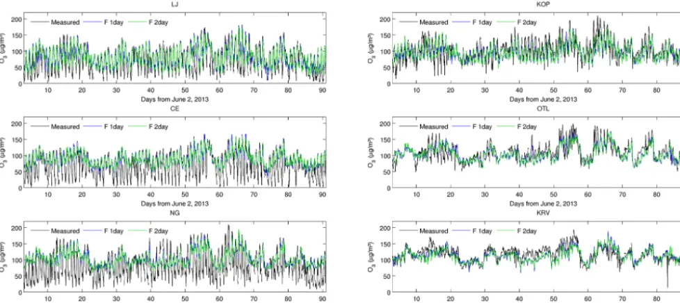
Table 2 shows conventional statistical scores evaluating the 1-day WRF-Chem forecast for the basic meteorological vari-ables: 2 m temperature (T2 m; for hourly values and daily maxima), 10 m wind speed (W10 m), RH and incoming SR. Results for three selected measuring sites (LJ, NG, MS) and the overall result for all 24 MET monitoring sites (shown in Fig. 3) are presented separately.
Incoming solar radiation is the main energy source that drives all atmospheric processes, including PBL processes, and has a critical role also in atmospheric chemistry. For al-most all sites the mean SR was overestimated by the model, with overall MEs of 16 and 11 W m−2for 1-day and 2-day forecasts, respectively. CORR was higher for 1-day (0.77) than for 2-day (0.71) forecasts, with a range of 0.64–0.90 for 1-day forecasts at different stations. The larger positive bias for the first day than for the second day can be attributed to less cloudy conditions during the first day of simulation.
fore-Table 2. Statistical scores for 1 h values of 2 m temperature (T2 m), 10 m wind speed (W10 m), relative humidity (RH), and for daily average
incoming solar radiation (SR). Shown are results for 1-day forecast, calculated separately for three measuring sites (LJ, NG, MS), and for 24 MET monitoring stations (ALL) during the 3-month period. In the case of temperature, results for daily maxima are also shown.
Variable Station No. cases Mean ME MAE RMSE CORR
T2 m 1 h (◦C) LJ 2129 20.3 −1.6 2.3 2.9 0.91 NG 2184 21.8 −1.1 2.1 2.5 0.94 MS 2184 19.2 −2 2.3 2.8 0.95 ALL 47 836 18.7 −1.3 2.3 2.9 0.93
T2 m max (◦C) LJ 89 26.5 −1.6 1.8 2.1 0.98
NG 90 26.8 −3 3 3.3 0.96
MS 90 26.2 −1.7 1.8 2 0.98 ALL 1976 24.2 −2.1 2.7 3.2 0.97
W10 m (m s−1) LJ 2129 1.5 0 0.7 1 0.58 NG 2183 2.7 1 1.4 1.9 0.35 MS 2184 2.3 0.4 1.1 1.4 0.53 ALL 43 378 2.4 0.8 1.4 1.9 0.36
RH (%) LJ 2066 62 −2 8 10 0.85
NG 2121 62 −1 12 15 0.75
MS 2121 69 3 8 11 0.88
ALL 48 556 68 2 11 14 0.77
SR (W m−2) LJ 90 276 19 31 43 0.84
NG 90 278 4 32 43 0.77
MS 90 273 15 26 37 0.9
ALL 1710 273 16 35 49 0.77
cast, which for particular stations can be positive (e.g. KRV) or negative (e.g. LJ and NG; Table 2).
Precipitation has an important role in cleansing of the at-mosphere by wet deposition and scavenging. On average, the predicted precipitation underestimated the measured 3-month accumulations by−55 mm (1-day) or−8 mm (2-day forecast), where the station-averaged, predicted 3-month pre-cipitation was 145 mm for 1-day and 194 mm for 2-day fore-casts (results not shown). It must also be taken into account that the 3.4.1 model version does not allow including the in-formation about hydrometeors at the boundaries of the nested domain (in the applied 1-way nesting procedure), which con-tributes to the negative simulated bias of precipitation. A large decrease in the precipitation bias from day 1 to day 2 suggests that different initialization methodology (e.g. using 1-day spin-up for meteorology) could improve the prediction of precipitation events.
3.2 Evaluation of air quality variables
In this section we evaluate WRF-Chem predictions for O3, NO2and PM10, as three of the most problematic pollutants in terms of harm to human health and compliance with EU limit values (EEA, 2012). Table 3 shows the domain-wide perfor-mance statistics for 1-day and 2-day forecasts of these pollu-tants where, in the case of O3, 1 h and 8 h averages and daily maxima are analysed separately. The comparison of 1-day
and 2-day forecasts shows that concentrations of air pollu-tants were somewhat better forecasted 1-day ahead by means of almost all of statistics shown in Table 3, with higher im-pact on O3predictions. Although the 2-day prediction was generally not worse for the majority of meteorological vari-ables, the reason for a better 1-day prediction in the case of O3 could be the somewhat stronger simulated winds on the second day of simulation. Stronger winds impact the trans-port and dispersion of pollutants and have the greatest con-sequence on secondary pollutants (like O3)which need time to be formed.
Table 3. Domain-wide performance statistics for 1-day and 2-day forecasts (in µg m−3). Results for all hourly (hour), 8 h averages (8 h), 8 h daily maximum (8 h max), daily maximum (max) and daily average (day) concentrations are shown.
No. cases Mean ME MAE RMSE CORR
O3(hour) 1 day 28 391 94.8 14.5 25.1 32.1 0.65 2 day 28 391 95.0 14.5 25.5 32.5 0.64
O3(8 h) 1 day 28 072 94.8 14.6 22.6 28.1 0.69 2 day 28 072 95.0 14.6 23.0 28.5 0.68
O3(8 h max) 1 day 1157 111.5 −0.1 13.2 16.5 0.77 2 day 1157 111.6 −0.2 13.7 17.0 0.75
O3(max) 1 day 1170 116.5 −2.7 13.3 16.7 0.81 2 day 1170 116.6 −3.1 14.0 17.5 0.78
NO2(hour) 1 day 26 178 7.3 −5.1 7.5 10.8 0.3 2 day 26 178 7.5 −4.9 7.6 10.8 0.3
PM10(day) 1 day 718 29.0 7.1 12.0 18.8 0.34 2 day 718 29.1 7.2 12.0 19.1 0.37
2006; Chuang et al., 2011; Yahya et al., 2014), which could be to some extent related to higher model resolution.
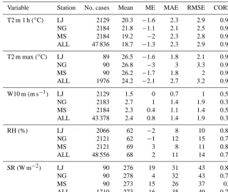
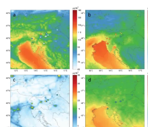
To understand results of the domain-wide statistics (in Ta-ble 3) we further analyse spatial and temporal characteristics of model O3predictions. Figure 4 shows a spatial pattern of average, simulated 1-day predictions for O3, NO2and PM10 overlaid with measured averages where, in the case of O3, results for all hourly values and for daily maxima are shown separately. Examples of forecasted and measured time series for O3 at different stations are shown in Fig. 5. In Fig. 4a the elevated alpine KRV station is the only one with a high negative bias (−12 µg m−3)in forecasted 1 h O3 concentra-tions at the lowest model layer, which can be explained by the too low altitude of the KRV station in model topography. The high negative bias for hourly O3 concentrations at the KRV station is reduced to a value of only−2 µg m−3by using the fifth model layer concentrations as explained in Sect. 2.3. The fifth model level predictions will be used for KRV in all analyses that follow. Besides KRV, the Mediterranean KOP and OTL stations, as well as the rural ZAV site, are sta-tions with comparatively high measured nighttime O3 lev-els, which results in a low overall bias for all hourly O3 val-ues for these stations (from−2 to−7 µg m−3). Namely, the WRF-Chem model cannot capture well the profound night-time O3reductions (shown also by Žabkar et al., 2013; Im et al., 2015a), which contributes to the overall overprediction of hourly O3concentrations (from 10 to 36 µg m−3) for sta-tions with very low measured nighttime O3concentrations. For sites with the highest positive bias in 1 h O3 concentra-tions (TRB, ZAG, HRA and ISK, with bias of 36, 31, 26 and 32 µg m−3, respectively), this can also be partly explained by the too high altitude of the stations in model orography (Table 1), since the mean O3 concentration increases with height.
Figure 4. The 3-month average 1-day predictions of (a) hourly O3, (b) O3daily maximum, (c) hourly NO2, and (d) daily PM10 con-centrations for the first model layer, overlaid with measurements.
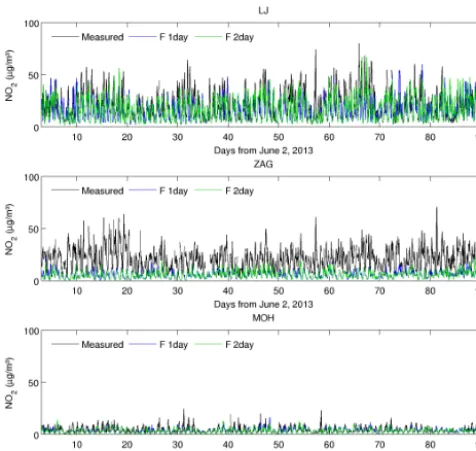
over-Figure 5. Time evolution of hourly ozone concentrations for 1-day (F 1 day) and 2-day (F 2 day) WRF-Chem predictions and measurements
for some stations during the 3-month period.
predicts O3daily maxima for 14 µg m−3. For other subalpine stations the bias of O3daily maxima predictions is lower.
To some extent the previously mentioned model over-predictions of nighttime O3 minima could be explained by model error in predicted NO2 levels. When evaluating the primary pollutants one must be aware that in the model the instantaneous emissions are spread over an entire grid box, which results in underestimated emissions and concentra-tions close to the source regions and overestimated emissions and concentrations at rural locations adjacent to the source regions, and can thus cause a combined effect of negative and positive biases at urban and rural sites. Comparisons of WRF-Chem-predicted NO2levels with measurements show that in spite of the high spatial resolution the concentrations of the small urban areas are insufficiently represented by the model (Fig. 4c). In Slovenia many towns are located in basins or very narrow valleys, usually poorly or, in some cases, not resolved in model topography. Smoothed local emissions for these towns show significant underestimations of NO2 con-centrations (e.g. ZAG in Fig. 6). In combination with poorly reproduced meteorological processes (calm and stable night-time conditions in valleys and basins) this results in an un-derestimation of the O3 loss by titration. This can explain the positive nighttime bias of O3 found at these sites. The situation is better for bigger cities, located in wider basins, like LJ or CE (LJ; Fig. 6), while at rural sites NO2is either well simulated (e.g. MOH; Fig. 6) or slightly overpredicted due to increased emissions from adjacent urban areas (e.g. ZAD; Fig. 6). The overall agreement of hourly NO2 predic-tions with measurements was good for rural sites while ur-ban sites experienced underpredictions, which were highest
for small cities, especially for NG (ME of−13 µg m−3)and ZAG (ME of−14 µg m−3).
dur-Figure 6. The same as Fig. 5 but for NO2at the LJ, ZAG and MOH stations.
ing the first heat wave episode (17–22 June), when during the hot and low wind conditions (after 17 June) the PM10 levels started to build up in the PBL over entire domain D2 (and over southwestern parts of domain D1) and reached the maximum concentrations in Slovenia again with prefrontal advection of polluted air masses. Both overpredictions con-tributed to an overall positive bias in forecasted PM10 con-centrations. Detailed analyses showed that high concentra-tions in domain D1 originated from boundary condiconcentra-tions, and appear to be a consequence of overestimated advection of Sa-haran dust in MOZART model predictions. The increase in PM10 concentrations over Slovenia was also simulated dur-ing the prefrontal advection related to the cold front which terminated the next two heat wave events in July and August (days 56 and 57 and days 67 and 68 in Fig. 7); however, dur-ing these days the predicted PM10 levels were close to the measured PM10concentrations.
3.3 Evaluation and comparison of different methods for O3daily maximum predictions
In this section we want to answer the question: how accurate is the 1 h O3daily maximum WRF-Chem forecast in compar-ison to the statistical model prediction or to persistence? Ac-cording to Zhang et al. (2012a) statistical models are known to be generally more suitable for complex site-specific re-lations between concentrations of air pollutants and predic-tors. With appropriate and accurate predictors they have a higher accuracy as compared to deterministic models which is along with their computational efficiency their main ad-vantage (Zhang et al., 2012a). Among the strengths of the deterministic models are that they give prognostic time- and
Figure 7. The same as Fig. 5 but for daily PM10concentrations at the MS and ZAD stations.
spatially resolved concentrations under typical and atypical scenarios and can give scientific insights into pollutant for-mation processes (Zhang et al., 2012a). Furthermore, they also allow for forecasts in locations which are not monitored due to their complete spatial coverage. In spite of simplified descriptions of physical and chemical processes in the deter-ministic models and inaccuracies and uncertainties in model inputs (in particular the emissions), some previous studies already suggested that deterministic models can also have skills similar to statistical forecasting tools (e.g. Manders et al., 2009). In addition to evaluation and comparison of O3 daily maxima predictions with WRF-Chem and the statisti-cal model, we decided to add a persistence model as a thresh-old for useful model prediction. Persistence works well under stationary conditions but, because it cannot handle changes in weather and emissions, fails at the beginning and at the end of the episodes (Zhang et al., 2010a). Regarding the ex-tremes, models of all types are known to have problems to accurately predict them, while persistence predicts extremes with a 1-day (2-day) time lag.
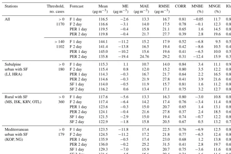
Table 4. Discrete evaluation of 1 h daily maximum ozone predictions (PER: persistence).
Stations Threshold, Forecast Mean ME MAE RMSE CORR MNBE MNGE IOA no. cases (µg m−3) (µg m−3) (µg m−3) (µg m−3) (%) (%)
All >0 F 1 day 116.5 −2.6 13.3 16.7 0.81 −0.05 11.7 0.86 1170 F 2 day 116.6 −3.1 14.0 17.5 0.78 −0.1 12.3 0.84 PER 1 day 119.5 −0.4 15.8 21.1 0.65 1.6 14.5 0.81 PER 2 day 119.8 −0.4 21.7 27.7 0.39 2.8 19.6 0.65 >140 F 1 day 144.1 −11.2 15.2 17.9 0.52 −6.8 9.5 0.57 1102 F 2 day 141.4 −13.8 16.5 19.4 0.42 −8.6 10.5 0.48 PER 1 day 145.0 −10.2 15.6 19.6 0.41 −6.5 10.0 0.52 PER 2 day 135.8 −19.4 24.76 29.2 0.31 −12.4 15.9 0.38 Subalpine >0 F 1 day 115.3 1.1 10.7 14.0 0.84 3.4 11.1 0.91 urban with SF 180 F 2 day 115.4 0.8 12.0 15.2 0.80 3.5 12.2 0.88 (LJ, HRA) PER 1 day 114.3 −0.3 16.7 21.7 0.64 2.2 16.5 0.80 PER 2 day 114.6 −0.3 21.9 27.8 0.41 3.9 21.6 0.65 SF 1 day 114.0 −0.5 11.9 15.7 0.81 1.6 11.2 0.88 SF 2 day 116.2 0.6 13.4 17.1 0.75 3.2 12.7 0.84
Rural with SF >0 F 1 day 117.6 −5.6 13.3 16.3 0.80 −3.0 10.8 0.86 (MS, ISK, KRV, OTL) 360 F 2 day 117.4 −6.4 14.2 17.4 0.76 −3.4 11.4 0.84 PER 1 day 123.6 −0.3 15.0 20.7 0.65 1.4 13.1 0.81 PER 2 day 124.1 −0.4 21.6 27.8 0.37 2.4 18.5 0.64 SF 1 day 121.5 −2.9 15.0 19.4 0.74 −0.7 12.2 0.83 SF 2 day 122.9 −1.8 15.8 20.5 0.67 0.5 13.2 0.79 Mediterranean >0 F 1 day 123.5 −11.8 17.4 22.5 0.76 −6.9 12.5 0.80 urban with SF 179 F 2 day 124.5 −11.2 17.2 21.8 0.77 −6.5 12.4 0.82 (KOP, NG) PER 1 day 135.9 −0.5 17.4 23.0 0.68 1.2 13.8 0.83 PER 2 day 136.0 −0.2 25.2 31.5 0.41 2.8 19.7 0.66 SF 1 day 129.3 −7.0 15.9 20.7 0.75 −3.6 11.6 0.83 SF 2 day 131.6 −4.5 15.6 20.4 0.74 −1.6 11.6 0.84
of atypical conditions not resolved by the statistical model. Looking at MAE and RMSE for all stations, except those with the highest ME (TRB, KOP), the WRF-Chem outper-forms the persistence already in the 1-day forecast. Among sites with available statistical forecasts there are only two (OTL, KOP) with WRF-Chem performing worse than the statistical forecast. CORR is one of the parameters that sug-gest how much the model is able to follow the true nature of processes regardless of the possible bias. For almost all stations WRF-Chem shows higher CORR than persistence for 1-day and 2-day forecasts. Only at the KRV station does the 1-day statistical forecast (CORR=0.80) somewhat out-perform WRF-Chem (0.74), and at NG and KOP the CORR values for WRF-Chem and the statistical model are very sim-ilar.
The Taylor diagrams in Fig. 9 show CORR together with the centred root-mean-square difference (RMSD) between model forecasts and observations, and the amplitude of their variations (standard deviation). The ideal model would have a correlation coefficient of 1 and a standard deviation equal to the observations, which means that it would be co-located with the black dot on the diagram. WRF-Chem gives higher CORR and lower RMSD for all types of stations, while the standard deviation of WRF-Chem O3daily maxima predic-tions is underestimated and lower than for other model
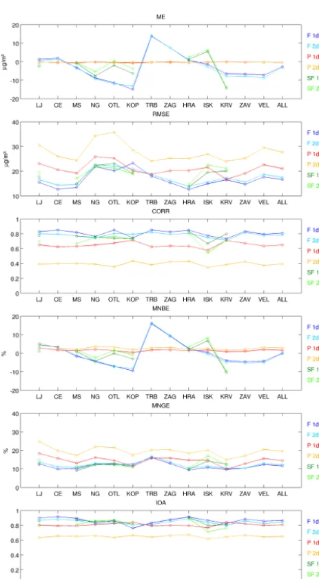
Figure 8. Site-by-site comparison of discrete statistics for 1-day and
2-day WRF-Chem (F 1 day, F 2 day), statistical (SF 1 day, SF 2 day) and persistence model (P 1 day, P 2 day) predictions of ozone daily maxima during the 3 summer months analysed.
in model topography, was compensated by taking predictions from the fifth model level.
The key requirement for a forecast system is to be able to predict O3concentration levels greater than a given thresh-old. Thus, in addition to the discrete evaluation just pre-sented, the contingency-table-based statistics are also an im-portant metric of forecast performance. Table 5 summarizes the categorical evaluation results for three different thresh-olds (120, 140, 160 µg m−3) of elevated O3 levels, which pose a greater risk to human health. Namely, it is impor-tant to take into account that results of categorical statistics are very sensitive to the threshold chosen, as well as to the overall pollution levels during the analysed months. Equi-table threat score (ETS) measures the fraction of observed
Figure 9. Taylor diagrams comparing 1-day and 2-day ozone daily
maximum statistical forecast (SF), persistence (P) and WRF-Chem forecast (F) for (a) subalpine urban stations with SF (LJ, HRA),
(b) subalpine urban stations without SF (CE, TRB, ZAG, VEL), (c) rural stations with SF (MS, ISK, KRV, OTL) and (d)
Mediter-ranean urban stations (NG, KOP).
under-Table 5. Categorical evaluation of 1 h daily maximum ozone predictions for different thresholds, calculated for eight monitoring sites with
available statistical forecast.
Threshold Forecast ETS CSI B FAR POD a b c d
>120 F 1 day 0.42 0.63 0.81 0.13 0.70 39 253 313 107 F 2 day 0.39 0.61 0.79 0.14 0.68 41 245 303 115 PER 1 day 0.31 0.59 0.99 0.25 0.74 91 267 249 93 PER 2 day 0.17 0.49 1.00 0.34 0.65 123 235 209 124 SF 1 day 0.42 0.67 1.02 0.21 0.81 67 257 243 61 SF 2 day 0.38 0.65 1.03 0.23 0.80 77 264 225 66
>140 F 1 day 0.40 0.50 0.64 0.15 0.551 19 111 490 92 F 2 day 0.37 0.47 0.66 0.19 0.53 25 108 476 95 PER 1 day 0.40 0.53 1.00 0.31 0.69 62 141 435 62 PER 2 day 0.19 0.35 1.00 0.48 0.52 97 106 391 97 SF 1 day 0.30 0.43 0.73 0.29 0.52 40 99 398 91 SF 2 day 0.30 0.43 0.70 0.27 0.51 37 98 403 94
>160 F 1 day 0.19 0.22 0.38 0.34 0.25 10 19 626 57 F 2 day 0.17 0.20 0.34 0.35 0.22 9 17 619 59 PER 1 day 0.40 0.45 1.00 0.38 0.62 29 47 595 29 PER 2 day 0.22 0.28 1.00 0.56 0.43 43 33 572 43 SF 1 day 0.23 0.27 0.49 0.35 0.32 13 24 539 52 SF 2 day 0.25 0.29 0.63 0.41 0.37 19 27 540 46
predict O3threshold exceedances shows as aB below 1 for these two models. The false alarm ratio (FAR) that measures the percentage of forecasted high O3events that turn out to be false alarms gives the highest skill to WRF-Chem, followed by the statistical model and persistence. The probability of detection (POD) is a measure of how often a high threshold occurrence is actually predicted to occur and is relatively low for WRF-Chem with respect to other models.
It must be noted that in categorical evaluations systematic biases like those obtained with WRF-Chem for some stations (e.g. KOP) significantly impact the model performance. For example, if the KOP station was excluded from categorical evaluations, WRF-Chem performance improved by means of all statistical measures (results not shown). If correction tech-niques, based on observations and the previous day’s forecast (e.g. McKeen et al., 2005, 2007; Kang et al., 2008), were to be applied to correct the systematic biases, WRF-Chem fore-casts might outperform the other two models even in categor-ical evaluations.
4 Summary and conclusion
A high resolution modelling system based on an online cou-pled WRF-Chem has been applied for numerical weather prediction and for forecasting air quality in Slovenia. In the study, the evaluation of the forecasting system has been con-ducted for 3 summer months. Since the selection of physical or chemical parameterization schemes influences and pos-sibly changes the outcomes, we decided to apply schemes which are well documented and have previously been used
in other applications (e.g. AQMEII). Both 1-day and 2-day predictions of meteorological and air quality variables have been analysed. The focus has been on O3 as it is the only pollutant with recorded exceedances of the legislation’s limit values during the three heat wave events in June, July and August 2013. WRF-Chem daily O3 maximum predictions have also been compared to the operational statistical model and persistence forecasts to answer the question of how skill-ful are the WRF-Chem model predictions in comparison to these two other models.
The 1-day and 2-day WRF-Chem PM10 forecasts showed a very low bias. Exceptions were two events with signifi-cantly overpredicted PM10levels due to prefrontal advection of polluted air masses from neighbouring regions. Knowing that the majority of the current chemical transport models show large negative biases in simulated PM10concentrations, these results present a good starting point for studying the importance of aerosol feedbacks with realistic model aerosol concentrations, left for future research.
Evaluations of predicted 1 and 8 h daily O3maxima, which are in the case of this pollutant of the highest interest, show good WRF-Chem model performance. Nevertheless, there are also stations which experience high over- or underpredic-tions of O3daily maximum levels. For Mediterranean sites the underpredictions of the daily maxima are most proba-bly due to inaccurate representation of costal processes in the model, which are crucial for the PBL height evolution and accumulation of pollution in the near-ground air layers. For some subalpine stations the reason for the higher bias in O3daily maximum predictions is their location either at el-evated mountainous or coastal regions or in narrow valleys which cannot be appropriately resolved in the current model resolution – which impacts how accurately a model simu-lates the local processes responsible for the level of local pollution. Comparisons of WRF-Chem O3 daily maximum forecasts with persistence and with statistical model
Appendix A: Statistical measures
Forith observed (Oi)and the corresponding modelled (Mi)
value of variable, discrete statistical measures are calculated as follows.
Mean error:
ME= 1 N
N
X
i=1
(Mi−Oi) .
Mean absolute error:
MAE= 1 N
N
X
i=1
|Mi−Oi|.
Root mean square error:
RMSE= v u u t
1
N
N
X
i=1
(Mi−Oi)2.
Correlation coefficient:
r= PN
i=1 Mi−M
Oi−O
q
PN
i=1 Mi−M
2
Oi−O
2.
Index of agreement:
IOA=1−
PN
i=1(Mi−Oi)2
PN i=1
Mi−O
+
Oi−O
2.
Mean normalized bias error:
MNBE= 1 N
N
X
i=1
Mi−Oi
Oi
×100.
Mean normalized gross error:
MNGE= 1 N
N
X
i=1
|Mi−Oi|
Oi
×100.
For categorical evaluation, all model predictions are first classified into four groups (a,b,candd):
1. prediction is above, but observation is below the thresh-old;
2. prediction and observation are above the threshold; 3. prediction and observation are below the threshold; 4. prediction is below, but observation is above the
thresh-old.
Categorical statistics are calculated as follows. Equitable threat score: ETS= b−ar
a+b+d−ar, where ar=
(a+b)(b+d) a+b+c+d .
Critical success index: CSI= b
a+b+d.
Bias:B=a+b
b+d.
False alarm ratio: FAR= a
a+b.
Probability of detection: POD= b
Acknowledgements. Centre of Excellence for Space Sciences and
Technologies SPACE-SI (OP13.1.1.2.02.0004) is in part financed by the European Union, European Regional Development Fund and the Republic of Slovenia, Ministry of Education, Science and Sport. The authors thankfully acknowledge TNO for providing the TNO-MACC-II anthropogenic emissions. Statistical model predictions and measurement data used in the study were kindly provided by the Slovenian Environmental Agency and Electroin-stitute Milan Vidmar. The support through COST Action ES1004 EuMetChem is gratefully acknowledged.
Edited by: R. Sander
References
Ackermann, I. J., Hass, H., Memmesheimer, M., Ziegenbein, C., and Ebel, A.: The parameterization of the sulfate-nitrate-ammonia aerosol system in the long-range transport model EU-RAD, Meteorological Atmospheric Physics, 57, 101–114, 1995. ALADIN International Team, The ALADIN project: Mesoscale modelling seen as a basic tool for weather forecasting and at-mospheric research, WMO Bull., 46, 317–324, 1997.
Baklanov, A.: Chemical weather forecasting: a new concept of in-tegrated modeling. Adv. Sci. Res., 4, 23–27, 2010.
Baklanov, A., Korsholm, U., Mahura, A., Petersen, C., and Gross, A.: Enviro-HIRLAM: on-line coupled modelling of urban mete-orology and air pollution, Adv. Sci. Res., 2, 41–46, 2008. Baklanov, A., Schlünzen, K., Suppan, P., Baldasano, J., Brunner,
D., Aksoyoglu, S., Carmichael, G., Douros, J., Flemming, J., Forkel, R., Galmarini, S., Gauss, M., Grell, G., Hirtl, M., Joffre, S., Jorba, O., Kaas, E., Kaasik, M., Kallos, G., Kong, X., Ko-rsholm, U., Kurganskiy, A., Kushta, J., Lohmann, U., Mahura, A., Manders-Groot, A., Maurizi, A., Moussiopoulos, N., Rao, S. T., Savage, N., Seigneur, C., Sokhi, R. S., Solazzo, E., Solomos, S., Sørensen, B., Tsegas, G., Vignati, E., Vogel, B., and Zhang, Y.: Online coupled regional meteorology chemistry models in Europe: current status and prospects, Atmos. Chem. Phys., 14, 317–398, doi:10.5194/acp-14-317-2014, 2014.
Balzarini, A., Pirovano, G., Honzak L., Žabkar, R., Curci, G., Forkel R., Hirtl, M., San José, R., Tuccella, P., and Grell, G.: WRF-Chem model sensitivity to chemical mechanisms choice in re-constructing aerosol optical properties, Atmos. Environ., 115, 604–619, doi:10.1016/j.atmosenv.2014.12.033, 2015.
Baró, R., Jiménez-Guerrero, P., Balzarini, A., Curci, G., Forkel, R., Hirtl, M., Honzak, L., Im, U., Lorenz, C., Pérez, J. L., Pirovano, G., San José, R., Tuccella, P., Werhahn, J., and Žabkar, R.: Sen-sitivity analysis of the microphysics scheme in WRF-Chem con-tributions to AQMEII phase 2., Atmos. Environ., 115, 620–629, doi:10.1016/j.atmosenv.2015.01.047, 2015.
Bocquet, M., Elbern, H., Eskes, H., Hirtl, M., Žabkar, R., Carmichael, G. R., Flemming, J., Inness, A., Pagowski, M., Pérez Camaño, J. L., Saide, P. E., San Jose, R., Sofiev, M., Vira, J., Baklanov, A., Carnevale, C., Grell, G., and Seigneur, C.: Data assimilation in atmospheric chemistry models: current status and future prospects for coupled chemistry meteorology models, At-mos. Chem. Phys., 15, 5325–5358, doi:10.5194/acp-15-5325-2015, 2015.
Byun, D. W. and Schere, K. L.: Review of the governing equations, computational algorithms, and other components of the Models – 3 Community Multiscale Air Quality (CMAQ) Modeling Sys-tem, Appl. Mech. Rev., 59, 51–77, 2006.
Chapman, E. G., Gustafson Jr., W. I., Easter, R. C., Barnard, J. C., Ghan, S. J., Pekour, M. S., and Fast, J. D.: Coupling aerosol-cloud-radiative processes in the WRF-Chem model: Investigat-ing the radiative impact of elevated point sources, Atmos. Chem. Phys., 9, 945–964, doi:10.5194/acp-9-945-2009, 2009.
Chen, F. and Dudhia, J.: Coupling an Advanced Land Surface– Hydrology Model with the Penn State NCAR MM5 Model-ing System. Part I: Model Implementation and Sensitivity, Mon. Weather Rev., 129, 569–585, 2001.
Chuang, M. T., Zhang, Y., and Kang, D. W.: Application of WRF-Chem-MADRID for real-time air quality forecasting over the southeastern United States, Atmos. Environ., 45, 6241–6250, 2011.
Cobourn, W. G.: Accuracy and reliability of an automated air qual-ity forecast system for ozone in seven Kentucky metropolitan area, Atmos. Environ., 41, 5863–5875, 2007.
Curci, G., Hogrefe, C., Bianconi, R., Im, U., Balzarini, A., Baro, R., Brunner, D., Forkel, R., Giordano, L., Hirtl, M., Honzak, L., Jimenez-Guerrero, P., Knote, C., Langer, M., Makar, P. A., Pirovano, G., Perez, J. L., San Jose, R., Syrakov, D., Tuccella, P., Werhahn, J., Wolke, R., Zabkar, R., Zhang, J., and Gal-marini, S.: Uncertainties of simulated aerosol optical properties induced by assumptions on aerosol physical and chemical prop-erties: an AQMEII-2 perspective, Atmos. Environ., 115, 541– 552, doi:10.1016/j.atmosenv.2014.09.009, 2015.
Eder, B. K., Kang, D., Mathur, R., Yu, S., and Schere, K.: An oper-ational evaluation of the Eta-CMAQ air quality forecast model, Atmos. Environ., 40, 4894–4905, 2006.
EEA: Air Quality in Europe – 2012 Report, ISBN 978-92-9213-328-3, Luxembourg: Office for Official Publications of the Euro-pean Union, 108 pp., 2012.
Emmons, L. K., Walters, S., Hess, P. G., Lamarque, J.-F., Pfister, G. G., Fillmore, D., Granier, C., Guenther, A., Kinnison, D., Laepple, T., Orlando, J., Tie, X., Tyndall, G., Wiedinmyer, C., Baughcum, S. L., and Kloster, S.: Description and evaluation of the Model for Ozone and Related chemical Tracers, version 4 (MOZART-4), Geosci. Model Dev., 3, 43–67, doi:10.5194/gmd-3-43-2010, 2010.
ENVIRON: CAMx User’s Guide, Comprehensive Air Quality Model With Extensions Version 5.40, ENVIRON International Corporation, Novato, California, 2011.
Fast, J., Aiken, A. C., Allan, J., Alexander, L., Campos, T., Cana-garatna, M. R., Chapman, E., DeCarlo, P. F., de Foy, B., Gaffney, J., de Gouw, J., Doran, J. C., Emmons, L., Hodzic, A., Herndon, S. C., Huey, G., Jayne, J. T., Jimenez, J. L., Kleinman, L., Kuster, W., Marley, N., Russell, L., Ochoa, C., Onasch, T. B., Pekour, M., Song, C., Ulbrich, I. M., Warneke, C., Welsh-Bon, D., Wied-inmyer, C., Worsnop, D. R., Yu, X.-Y., and Zaveri, R.: Eval-uating simulated primary anthropogenic and biomass burning organic aerosols during MILAGRO: implications for assessing treatments of secondary organic aerosols, Atmos. Chem. Phys., 9, 6191–6215, doi:10.5194/acp-9-6191-2009, 2009.
radia-tive forcing in the vicinity of Houston using a fully coupled meteorology-chemistry-aerosol model, J. Geophys. Res., 111, D21305, doi:10.1029/2005JD006721, 2006.
Forkel, R., Werhahn, J., Buus Hansen, A., McKeen, S., Peckham, S., Grell, G., and Suppan, P.: Effect of aerosol-radiation feedback on regional air quality – A case study with WFR/Chem, Atmos. Environ., 53, 202–211, 2012.
Forkel, R., Balzarini, A., Baró, R., Curci, G., Jiménez-Guerrero, P., Hirtl, M., Honzak, L., Im, U., Lorenz, C., Pérez, J. L., Pirovano, G., San José, R., Tuccella, P., Werhahn, J., and Žabkar, R.: Analysis of the WRF-Chem contributions to AQMEII phase 2 with respect to aerosol radiative feedbacks on meteorol-ogy and pollutant distribution, Atmos. Environ., 115, 630–645, doi:10.1016/j.atmosenv.2014.10.056, 2015.
Grell, G. A. and Baklanov, A.: Integrated modeling for forecasting weather and air quality: A call for fully coupled approaches, At-mos. Environ., 45, 6845–6851, 2011.
Grell, G. A. and Devenyi, D.: A generalized approach to pa-rameterizing convection combining ensemble and data as-similation techniques, Geophys. Res. Lett., 29, 38.1–38.4, doi:10.1029/2002GL015311, 2002.
Grell, G. A., Dudhia, J., and Stauffer, D.: A description of the fifth-generation Penn State/NCAR Mesoscale model (MM5), TN-398+STR,NCAR, Boulder, CO, 1994.
Grell, G. A., Emeis, S., Stockwell, W. R., Schoenemeyer, T., Forkel, R., Michalakes, J., Knoche, R., andSeidl, W.: Application of a multiscale, coupled MM5/chemistry model to the complex terrain of the VOTALP valley campaign, Atmos. Environ., 34, 1435–1453, 2000.
Grell, G. A., Knoche, R., Peckham, S. E., and McKeen, S. A.: On-line versus offOn-line air quality modeling on cloud-resolving scales, Geophys. Res. Lett., 31, L16117, doi:10.1029/2004GL020175, 2004.
Grell, G. A., Peckham, S. E., Schmitz, R., McKeen, S. A., Frost, G., Skamarock, W., and Eder, B.: Fully coupled “online” chemistry within the WRF model, Atmos. Environ., 39, 6957–6975, 2005. Guenther, A., Karl, T., Harley, P., Wiedinmyer, C., Palmer, P. I., and Geron, C.: Estimates of global terrestrial isoprene emissions using MEGAN (Model of Emissions of Gases and Aerosols from Nature), Atmos. Chem. Phys., 6, 3181–3210, doi:10.5194/acp-6-3181-2006, 2006.
Hong, S., Noh, Y., and Dudhia, J.: A new vertical diffusion pack-age with an explicit treatment of entrainment processes, Mon. Weather Rev., 134, 2318–2341, 2006.
Hu, X.-M., Doughty, D., Sanchez, K. J., Joseph, E., and Fuentes, J. D.: Ozone variability in the atmospheric boundary layer in Mary-land and its implications for vertical transport model, Atmos. En-viron., 46, 354–364, 2012.
Iacono, M. J., Delamere, J. S., Mlawer, E. J., Shephard, M. W., Clough, S. A., and Collins, W. D.: Radiative forcing by long-lived greenhouse gases: Calculations with the AER radiative transfer models, J. Geophys. Res., 113, D13103, doi:10.1029/2008JD009944, 2008.
Im, U., Bianconi, R., Solazzo, E., Kioutsioukis, I., Badia, A., Balzarini, A., Baro, R., Bellasio, R., Brunner, D., Chemel, C., Curci, G., Flemming, J., Forkel, R., Giordano, L., Jimenez-Guerrero, P., Hirtl, M., Hodzic, A., Honzak, L., Jorba, O., Knote, C., Kuenen, J. J. P., Makar, P. A., Manders-Groot, A., Neal, L., Perez, J. L., Pirovano, G., Pouliot, G., San Jose,
R., Savage, N., Schroder, W., Sokhi, R. S., Syrakov, D., To-rian, A., Tuccella, P., Werhahn, K., Wolke, R., Yahya, K., Žabkar, R., Zhang, Y., Zhang, J., Hogrefe, C., and Galmarini, S.: Evaluation of operational online-coupled regional air qual-ity models over Europe and North America in the context of AQMEII phase 2. Part I: Ozone, Atmos. Environ., 115, 404–420, doi:10.1016/j.atmosenv.2014.09.042, 2015a.
Im, U., Bianconi, R., Solazzo, E., Kioutsioukis, I., Badia, A., Balzarini, A., Baro, R., Bellasio, R., Brunner, D., Chemel, C., Curci, G., Denier van der Gon, H. A. C., Flemming, J., Forkel, R., Giordano, L., Jimenez-Guerrero, P., Hirtl, M., Hodzic, A., Honzak, L., Jorba, O., Knote, C., Makar, P. A., Manders-Groot, A., Neal, L., Perez, J. L., Pirovano, G., Pouliot, G., San Jose, R., Savage, N., Schroder, W., Sokhi, R. S., Syrakov, D., Torian, A., Tuccella, P., Werhahn, K., Wolke, R., Yahya, K., Žabkar, R., Zhang, Y., Zhang, J., Hogrefe, C., and Galmarini, S.: Evalua-tion of operaEvalua-tional online-coupled regional air quality models over Europe and North America in the context of AQMEII phase 2. Part II: Particulate Matter, Atmos. Environ., 115, 404–420, doi:10.1016/j.atmosenv.2014.09.042, 2015b.
Jacobson, M. Z.: GATOR-GCMM: A global through urban scale air pollution and weather forecast model. 1. Model design and treatment of subgrid soil, vegetation, roads, rooftops, water, sea ice, and snow, J. Geophys. Res., 106, 5385–5402, 2001. Kaminski, J. W., Neary, L., Struzewska, J., McConnell, J. C., Lupu,
A., Jarosz, J., Toyota, K., Gong, S. L., Côté, J., Liu, X., Chance, K., and Richter, A.: GEM-AQ, an on-line global multiscale chemical weather modelling system: model description and eval-uation of gas phase chemistry processes, Atmos. Chem. Phys., 8, 3255–3281, doi:10.5194/acp-8-3255-2008, 2008.
Kang, D., Mathur, R., Rao, S. T., and Yu, S.: Bias adjustment tech-niques for improving ozone air quality forecasts, J. Geophys. Res., 113, D23308, doi:10.1029/2008JD010151, 2008.
Klein, T., Kukkonen, J., Dahl, A., Bossioli, E., Baklanov, A., Vik, A. F., Agnew, P., Karatzas, K. D., and Sofiev, M.: Interactions of Physical, Chemical, and Biological Weather Calling for an Inte-grated Approach to Assessment, Forecasting, and Communica-tion of Air Quality, AMBIO, 41, 851–864, 2012.
Kong, X., Forkel, R., Sokhi, R., Suppan, P., Baklanovc, A., Gauss, M., Brunner, D., Baro Esteban, R., Balzarini, A., Chemel, C., Curci, G., Galmarini, S., Jiménez Guerrero, P., Hirtl, M., Honzak, L., Im, U., Pérez, J. L., Piravano, G., San Jose, R., Schlünzen, H., Tsegas, G., Tuccella, P., Werhahn, J., and Žabkar, R.: In-vestigation of meteorology and chemistry interactions and their representations in online coupled models with the supported case Studies from AQMEII phase2, Atmos. Environ., 527–540, doi:10.1016/j.atmosenv.2014.09.020, 2015.
Li, G., Zavala, M., Lei, W., Tsimpidi, A. P., Karydis, V. A., Pan-dis, S. N., Canagaratna, M. R., and Molina, L. T.: Simulations of organic aerosol concentrations in Mexico City using the WRF-CHEM model during the MCMA-2006/MILAGRO campaign, Atmos. Chem. Phys., 11, 3789–3809, doi:10.5194/acp-11-3789-2011, 2011.
McCollister, G. and Wilson, K.: Linear stochastic models for fore-casting daily maxima and hourly concentrations of air pollutants, Atmos. Environ., 9, 417–423, 1975.
McKeen, S., Wilczak, J., Grell, G., Djalova, I., Peckham, S., Hsie, E.-Y., Gong, W., Bouchet, V., Ménard, S., Moffet, R., McHenry, J., McQueen, J., Tang, Y., Carmichael, G.R., Pagowski, M., Chan, A., Dye, t., Frost, G., Lee, P., and Mathur, R.: Assessment of an ensemble of seven real-time ozone forecasts over eastern North America during the summer of 2004, J. Geophys. Res., 110, D21307, doi:10.1029/2005JD005858, 2005.
McKeen, S., Chung, S. H., Wilczak, J., Grell, G., Djalalova, I., Peckham, S., Gong, W., Bouchet, V., Moffet, R., Tang, Y., Carmichael, G. R., Mathur, R., and Yu, S.: Evaluation of several PM2.5 forecast models using data collected during the ICARTT/NEAQS 2004 field study, J. Geophys. Res., 112, D10S20, doi:10.1029/2006JD007608, 2007.
McKeen, S., Grell, G., Peckham, S., Wilczak, J., Djalalova, I., Hsie, E.-Y., Frost, G., Peischl, J., Schwarz, J., Spackman, R., Holloway, J., de Gouw, J., Warneke, C., Gong, W., Bouchet, V., Gaudreault, S., Racine, J., McHenry, J., McQueen, J., Lee, P., Tang, Y., Carmichael, G. R., and Mathur, R.: An evalua-tion of real-time air quality forecasts and their urban emissions over eastern Texas during the summer of 2006 Second Texas Air Quality Study field study, J. Geophys. Res., 114, D00F11, doi:10.1029/2008JD011697, 2009.
Menut, L., Bessagnet, B., Khvorostyanov, D., Beekmann, M., Blond, N., Colette, A., Coll, I., Curci, G., Foret, G., Hodzic, A., Mailler, S., Meleux, F., Monge, J.-L., Pison, I., Siour, G., Turquety, S., Valari, M., Vautard, R., and Vivanco, M. G.: CHIMERE 2013: a model for regional atmospheric composition modelling, Geosci. Model Dev., 6, 981–1028, doi:10.5194/gmd-6-981-2013, 2013.
Misenis, C. and Zhang, Z.: An examination of sensitivity of WRF-Chem predictions to physical parameterizations, horizontal grid spacing, and nesting options, Atmos. Res., 97, 315–334, 2010. Moody, J. and Galloway, J.: Quantifying the relationship between
atmospheric transport and the chemical composition of precipi-tation on Bermuda, Tellus B, 40, 436–479, 1988.
Morrison, H., Thompson, G., and Tatarskii, V.: Impact of cloud mi-crophysics on the development of trailing stratiform precipitation in a simulated squall line: Comparison of one- and two-moment schemes, Mon. Weather Rev., 137, 991–1007, 2009.
Otte, T. L., Pouliot, G., Pleim, J. E., Young, J. O., Schere, K. L., Wong, D. C., Lee, P. C. S., Tsidulko, M., McQueen, J. T., David-son, P., Mathur, R., Chuang, H.-Y., DiMego, G., and Seaman, N. L.: NCEP Notes: linking the Eta model with the community mul-tiscale air quality (CMAQ) modeling system to build a national air quality forecasting system, Weather Forecast., 20, 367–384, 2005.
Pagowski, M., Liu, Z., Grell, G. A., Hu, M., Lin, H.-C., and Schwartz, C. S.: Implementation of aerosol assimilation in Grid-point Statistical Interpolation (v. 3.2) and WRF-Chem (v. 3.4.1), Geosci. Model Dev., 7, 1621–1627, doi:10.5194/gmd-7-1621-2014, 2014.
Peckham, S. E., Grell, G. A., McKeen, S. A., Barth, M., Pfister, G., Wiedinmyer, C., Fast, J. D., Gustafson, W. I., Ghan, S. J., Za-veri, R., Easter, R. C., Barnard, J., Chapman, E., Hewson, M., Schmitz, R., Salzman, M., and Freitas, S. R.: WRF-Chem Ver-sion 3.3 User’s Guide, US Dept. of Commerce, National Oceanic
and Atmospheric Administration, Oceanic and Atmospheric Re-search Laboratories, Global Systems Division, 2012.
Pouliot, G., Pierce, T., Denier van der Gon, H. A. C., Kuenen, J., Zhang, J., Moran, M. D., and Makar, P. A.: Analysis of the emission inventories and model-ready emission datasets of Eu-rope and North America for phase 2 of the AQMEII project, At-mos. Environ., doi:10.1016/j.atmosenv.2014.10.061, online first, 2014.
Saide, P. E., Carmichael, G. R., Spak, S. N., Gallardo, L., Osses, A. E., Mena-Carrasco, M. A., and Pagowski, M.: Forecasting urban PM10and PM2.5pollution episodes in very stable nocturnal con-ditions and complex terrain using WRF-Chem CO tracer model, Atmos. Environ., 45, 2769–2780, 2011.
San Josè, R., Pèrez, J. L., Balzarini, A., Barò, R., Curci, G., Forkel, R., Galmarini, S., Grell, G., Hirtl, M., Honzak, L., Im, U., Jimènez-Guerrero, P., Langer, M., Pirovano, G., Tuccella, P., Werhahn, J., and Zabkar, R.: Sensitivity of feedback effects in CBMZ/MOSAIC chemical mechanism, Atmos. Environ., 115, 646–656, doi:10.1016/j.atmosenv.2015.04.030, 2015.
SEA: Upgrade of the system for monitoring air pollution, determin-ing the causes of excessive burdendetermin-ing and analysis of the effects of improvement measures, Project presentation, Slovenian En-vironment Agency, available at: http://www.arso.gov.si/en/, last access: 12 June 2014.
Schell, B., Ackermann, I. J., Hass, H., Binkowski, F. S., and Ebel, A.: Modeling the formation of secondary organic aerosol within a comprehensive air quality model system, J. Geophys. Res., 106, 28275–28293, 2001.
Shaw, W. J., Allwine, K., Fritz, B. G., Rutz, F. C., Rishel, J. P., and Chapman, E. G.: An evaluation of the wind erosion module in DUSTRAN, Atmos. Environ., 42, 1907–1921, 2008.
Skamarock, W. C., Klemp, J. B., Dudhia, J., Gill, D. O., Barker, D. M., Duda, M. G., Huang, X. Y., Wang, W., and Powers, J. G.: A Description of the Advanced Research WRF Version 3. NCAR Technical Note, NCAR/TN-475thSTR, 113 pp., 2008.
Stockwell, W. R., Middleton, P., Chang, J. S., and Tang, X.: The sec-ond generation regional acid deposition model chemical mech-anism for regional air quality modeling, J. Geophys. Res., 95, 16343–16367, 1990.
Sudo, K., Takahashi, M., Kurokawa, J., and Akimoto, H.: CHASER: A global chemical model of the tropo-sphere 1. Model description, J. Geophys. Res., 107, 4339, doi:10.1029/2001JD001113, 2002.
Takigawa, M., Niwano, M., Akimoto, H., and Takahashi, M.: Devel-opment of a One-way Nested Global-regional Air Quality Fore-casting Model, SOLA, 3, 081–084, 2007.
Taylor, K. E.: Summarizing multiple aspects of model performance in a single diagram, J. Geophys. Res., 106, 7183–7192, 2001. Tie, X., Geng, F. H., Peng, L., Gao, W., and Zhao, C. S.:
Measure-ment and modeling of O3variability in Shanghai, China; applica-tion of the WRF-Chem model, Atmos. Environ., 43, 4289–4302, 2009.
Tong, D. Q. and Mauzerall, D. L.: Spatial variability of summertime tropospheric ozone over the continental United States: Implica-tions of an evaluation of the CMAQ model, Atmos. Environ., 40, 3041–3056, 2006.
north-ern France and southnorth-ern England, J. Geophys. Res., 108, 4021, doi:10.1029/2000JD000301, 2003.
US EPA (US Environmental Protection Agency): Guidance for reg-ulatory application of the Urban Airshed Model, EPA-450/4-91-013, July 1991, United States Environmental Protection Agency, Research Triangle Park, NC 27711, 1991.
van Loon, M., Roemer, M. G. M., Builtjes, P. J. H., Bessagnet, B., Rouil, L., Christensen, J. H., Brandt, J., Fagerli, H., Tarrason, L., and Rodgers, I.: Model inter-comparison in the framework of the review of the unified EMEP model, Techical report R2004/282, TNO, 2004.
Vlachogianni, A., Kassomenos, P., Karppinen, A., Karakitsios, S., and Kukkonen, J.: Evaluation of a multiple regression model for the forecasting of the concentrations of NOxand PM10in Athens and Helsinki, Sci. Total Environ., 409, 1559–1571, 2011. Vogel, B., Vogel, H., Bäumer, D., Bangert, M., Lundgren, K., Rinke,
R., and Stanelle, T.: The comprehensive model system COSMO-ART – Radiative impact of aerosol on the state of the atmo-sphere on the regional scale, Atmos. Chem. Phys., 9, 8661–8680, doi:10.5194/acp-9-8661-2009, 2009.
Wild, O., Zhu, X., and Prather, M. J.: Fast-J: Accurate Simulation of In- and Below-Cloud Photolysis in Tropospheric chemical Mod-els, J. Atmos. Chem., 37, 245–282, 2000.
Wolff, G. T. and Lioy, P. J.: An empirical model for forecasting maximum daily ozone levels in the northeastern United States, J. Air Pollut. Control Assoc., 28, 1034–1038, 1978.
Yahya, K., Zhang, Y., and Vukovich, J. M.: Real-time air quality forecasting over the southeastern United States using WRF/Chem-MADRID: Multiple-year assessment and sensitiv-ity studies, Atmos. Environ., 92, 318–338, 2014.
Yang, Q., W. I. Gustafson Jr., Fast, J. D., Wang, H., Easter, R. C., Morrison, H., Lee, Y.-N., Chapman, E. G., Spak, S. N., and Mena-Carrasco, M. A.: Assessing regional scale predictions of aerosols, marine stratocumulus, and their interactions dur-ing VOCALS-REx usdur-ing WRF-Chem, Atmos. Chem. Phys., 11, 11951–11975, doi:10.5194/acp-11-11951-2011, 2011.
Zhang, Y.: Online-coupled meteorology and chemistry models: his-tory, current status, and outlook, Atmos. Chem. Phys., 8, 2895– 2932, doi:10.5194/acp-8-2895-2008, 2008.
Zhang, Y., Pan, Y., Wang, K., Fast, J. D., and Grell, G. A.: Chem-MADRID: incorporation of an aerosol module into WRF-Chem and its initial application to the TexAQS2000 episode, J. Geophys. Res., 115, D18202, doi:10.1029/2009JD013443, 2010a.
Zhang, Y., Wen, X.-Y., and Jang, C. J.: Simulating climate-chemistry-aerosol-cloud radiation feedbacks in continental U.S. using online-coupled WRF-Chem, Atmos. Environ., 44, 3568– 3582, 2010b.
Zhang, Y., Bocquet, M., Mallet, V., Seigneur, C., and Baklanov, A.: Real-time air quality forecasting, part I: History, techniques, and current status, Atmos. Environ., 60, 632–665, 2012a.
Zhang, Y., Bocquet, M., Mallet, V., Seigneur, C., and Baklanov, A.: Real-time air quality forecasting, part II: State of the science, current research needs, and future prospects, Atmos. Environ., 60, 656–676, 2012b.
Žabkar, R.: Nadgradnja modela statistiˇcnega napovedovanja ozona s predhodnim razvršˇcanjem trajektorij v skupine, final report, available at: http://www.arso.gov.si/zrak/kakovost%20zraka/ poro%C4%8Dila%20in%20publikacije/poro%C4%8Dila% 20o%20projektih/Porocilo_2011%20_napoved_ozona.pdf, 2011.
Žabkar, R., Rakovec, J., and Gaberšek, S.: A trajectory analysis of summertime ozone pollution in Slovenia, Geofizika, 25, 179– 202, 2008.
Žabkar, R., Rakovec, J., and Koraˇcin, D.: The roles of regional ac-cumulation and advection of ozone during high ozone episodes in Slovenia: a WRF-Chem modelling study, Atmos. Environ., 45, 1192–1202, 2011.