https://doi.org/10.5194/gmd-11-665-2018 © Author(s) 2018. This work is distributed under the Creative Commons Attribution 3.0 License.
The dynamical core of the Aeolus 1.0 statistical–dynamical
atmosphere model: validation and parameter optimization
Sonja Totz1,2, Alexey V. Eliseev1,3,4,5,6, Stefan Petri1, Michael Flechsig1, Levke Caesar1,2, Vladimir Petoukhov1, and Dim Coumou1,7
1Potsdam Institute for Climate Impact Research (PIK), Leibniz Foundation, Potsdam, Germany 2Department of Physics, Potsdam University, Potsdam, Germany
3A.M. Obukhov Institute of Atmospheric Physics RAS, Moscow, Russia 4Kazan Federal University, Kazan, Russia
5Institute of Applied Physics, Russian Academy of Sciences, Nizhny Novgorod, Russia 6Lomonosov Moscow State University, Faculty of Physics, Moscow, Russia
7Institute for Environmental Studies (IVM), Department of Water & Climate Risk, VU University Amsterdam, Amsterdam, the Netherlands
Correspondence:Sonja Totz ([email protected]) Received: 11 October 2016 – Discussion started: 2 December 2016
Revised: 14 November 2017 – Accepted: 11 December 2017 – Published: 22 February 2018
Abstract.We present and validate a set of equations for rep-resenting the atmosphere’s large-scale general circulation in an Earth system model of intermediate complexity (EMIC). These dynamical equations have been implemented in Aeo-lus 1.0, which is a statistical–dynamical atmosphere model (SDAM) and includes radiative transfer and cloud modules (Coumou et al., 2011; Eliseev et al., 2013). The statistical dynamical approach is computationally efficient and thus en-ables us to perform climate simulations at multimillennia timescales, which is a prime aim of our model development. Further, this computational efficiency enables us to scan large and high-dimensional parameter space to tune the model pa-rameters, e.g., for sensitivity studies.
Here, we present novel equations for the large-scale zonal-mean wind as well as those for planetary waves. Together with synoptic parameterization (as presented by Coumou et al., 2011), these form the mathematical description of the dy-namical core of Aeolus 1.0.
We optimize the dynamical core parameter values by tun-ing all relevant dynamical fields to ERA-Interim reanaly-sis data (1983–2009) forcing the dynamical core with pre-scribed surface temperature, surface humidity and cumulus cloud fraction. We test the model’s performance in repro-ducing the seasonal cycle and the influence of the El Niño– Southern Oscillation (ENSO). We use a simulated annealing
optimization algorithm, which approximates the global min-imum of a high-dimensional function.
With non-tuned parameter values, the model performs rea-sonably in terms of its representation of zonal-mean circula-tion, planetary waves and storm tracks. The simulated an-nealing optimization improves in particular the model’s rep-resentation of the Northern Hemisphere jet stream and storm tracks as well as the Hadley circulation.
The regions of high azonal wind velocities (planetary waves) are accurately captured for all validation experiments. The zonal-mean zonal wind and the integrated lower tropo-sphere mass flux show good results in particular in the North-ern Hemisphere. In the SouthNorth-ern Hemisphere, the model tends to produce too-weak zonal-mean zonal winds and a too-narrow Hadley circulation. We discuss possible reasons for these model biases as well as planned future model im-provements and applications.
1 Introduction
General circulation models (GCMs) are physically the most realistic tools for studying and modelling climate vari-ability and climate change in the Earth system. However, due to their relatively high resolution, they are costly in terms of CPU runtime, limiting their applicability to study climate variability over long (∼millennia) timescales.
On the other hand, highly idealized and computational ef-ficient models for the climate system are able to simulate long time periods, but those are often box or one- or two-dimensional models describing only a limited number of pro-cesses or feedbacks of the real world. Hence, their applica-tion is limited, but they have been applied to study paleocli-mate (Berger et al., 1992; Harvey, 1989) and future global change (Xiao et al., 1997).
A third class of models are so-called Earth system models of intermediate complexity (EMICs) which form a compro-mise between the computationally expensive (but more re-alistic) GCMs and the highly simplified models (Claussen et al., 2002). The number of processes and feedbacks are comparable to GCMs; however, due to a reduction in reso-lution and/or complexity of some model components, it is possible to study climate simulations up to multimillennia timescales (Eliseev et al., 2014a, b; Ganopolski et al., 2001; Montoya et al., 2005). Other applications include determin-ing quick assessments of climate change impacts or runndetermin-ing thousands of parameter sensitivity experiments (Knutti et al., 2002; Schmittner and Stocker, 1999).
EMICs are thus particularly useful for understanding the roles of different Earth components on very long timescales (multimillennia and longer) and consequently form useful tools complementary to GCMs. Internal climate processes on such very long timescales are primarily driven by ocean and ice dynamics (Holland et al., 2001; Latif, 1998; Polyakov et al., 2003), with the atmosphere’s role being likely limited to globally distributing any perturbations to the system. In GCMs, it is however often the atmosphere which takes most of the computational load due to the need to resolve syn-optic weather systems, which requires a high-resolution dis-cretization in space and time. For these reasons, a key step in the development of EMICs intended for studying ocean and ice dynamics on multimillennial timescales is the deriva-tion and validaderiva-tion of statistical–dynamical equaderiva-tions which accurately represent atmosphere dynamics (Coumou et al., 2011).
EMICs have been used in many climate studies and sev-eral different types of simplified atmospheric components that form part of an EMIC exist including two-dimensional, zonally averaged atmosphere models, 2.5-D atmosphere models (the vertical dimension is reconstructed using two-dimensional fields) with simple energy balance or statistical– dynamical atmosphere models (SDAMs) (Claussen et al., 2002; McGuffie and Henderson-Sellers, 2005). Most EMIC studies focus on climate variability on very long timescales (e.g., glacial cycles), and therefore fast processes are nor-mally parameterized. In particular, SDAMs parameterize
smaller-scale (and more short-lived) processes like synop-tic eddy activity in terms of the large-scale, long-term fields. The assumption of those models is thus that atmospheric variables can be expressed in separate terms of a large-scale, long-term component, with characteristic spatial and temporal scales of L >1000 km and T >10 days, and a small-scale component-like ensemble of synoptic-scale ed-dies and waves. The latter are then parameterized by their averaged statistical characteristics (their total kinetic energy and heat, their moist and momentum fluxes, etc.). This means that transport effects of the fast-moving weather systems on the large-scale, long-term atmospheric motion are averaged (Ehlers and Krafft, 2001).
The essential difference compared to GCMs is the point of truncation in the frequency spectrum of atmospheric mo-tion (Saltzman, 1978). GCMs solve all phenomena of fre-quencies lower than and including synoptic cyclones (and sometimes even mesoscale systems), whereas statistical– dynamical (SD) models parameterize all scales smaller than and equal to synoptic. Much of the difficulty in SD models is to define physically reasonable parameterizations occurring in the equations (Saltzman, 1978). For Aeolus, the synoptic parameterization has been described in detail in Coumou et al. (2011).
As written above, SD models are also spatially averaged since, for long-term climate simulations, we are typically in-terested in the large spatial aspects of the climate. It is fur-ther practical to split the large-scale, long-term field into two components: the zonally averaged mean field and the asym-metric departure of the field from the zonally averaged fields characterizing the east–west variations. The azonal variables can be, for example, resolved by one-dimensional Fourier components around latitude circles or into spherical harmon-ics (Saltzman, 1978).
Here, we present the Aeolus 1.0 dynamical core, devel-oped at the Potsdam Institute for Climate Impact Research (PIK), a new SD model for the atmosphere. It uses some as-pects of the atmosphere module of the EMIC CLIMBER-2 developed by Petoukhov et al. (2000). The dynamical core is completely new with novel equations for the large-scale meridional wind speed as well as quasi-stationary planetary waves. Together with the synoptic parameterizations pre-sented in Coumou et al. (2011), these equations form the new dynamical core of Aeolus 1.0. The model is coupled with the cloud module consisting of a three-layer stratiform plus con-vective cloud scheme as presented and validated in Eliseev et al. (2013).
ERA-Interim reanalysis data (climatology 1983–2009). The effects of parameter tuning are evaluated to improve the per-formance of the model.
In Sect. 2, we present the novel equations of the Aeo-lus 1.0 dynamical core with the derivation of these equa-tions presented in the Supplement (Sects. S1–S2). The dy-namical core is coupled with a convective plus three-layer stratiform cloud scheme (which includes low-level, mid-level and upper-level stratiform clouds) developed by Eliseev et al. (2013). In Sect. 3, we describe the experiment setup and the used reanalysis data sets. In Sect. 4, we explain the model discretization, and in Sect. 5 we introduce our specific cali-bration method. For parameter optimization of the wind ve-locities, we use simulated annealing, which approximates the global minimum of a high-dimensional function (Flechsig et al., 2013). In Sect. 6, we present Aeolus’ dynamical fields with pre-optimized and optimized parameters and compare them with observations and output from models of the Cou-pled Model Intercomparison Project phase 5 (CMIP5). We conclude by discussing performance and limitations of the model in Sect. 7.
2 Governing equations
2.1 General structure of the atmosphere
Aeolus 1.0 is a 2.5-D SD model, with the vertical dimen-sion being largely parameterized and only coarsely resolved, and it therefore belongs to the class of intermediate com-plexity atmosphere models. Water and energy conservation is achieved via a set of two-dimensional, vertically averaged prognostic equations for temperature and specific humidity (Petoukhov et al., 2000).
The three-dimensional structure is described by these two-dimensional surface fields with the vertical dimensions re-constructed using an equation for the lapse rate and assum-ing an exponential profile for specific humidity (Petoukhov et al., 2000).
For given temperature and specific humidity fields, the three-dimensional wind field is calculated using a set of diag-nostic equations. These statistical–dynamical equations for the wind fields are coupled and thus need several time steps or iterations to equilibrate.
The equations of the dynamical core of Aeolus 1.0 are separated into equations for the (1) synoptic-scale tran-sient waves (or storm tracks), (2) quasi-stationary planetary waves and (3) the zonal-mean wind. Thus, following clas-sical statistical–dynamical approaches (Dobrovolski, 2000; Imkeller and von Storch, 2012), the key assumption is that the wind velocity field V can be split into a synoptic-scale component V0 (2- to 6-day period) and a large-scale, long-term componenthVi(Fraedrich and Böttger, 1978) such that V = hVi +V0= {hui,hvi,hwi} +u0, v0, w0 . (1)
The variablesu,vandwdescribe the wind velocity in zonal, meridional and vertical directions. The brackets (h. . .i) sym-bolize time-averaged quantities and the prime (. . .0)
indi-cates deviations from this time-averaged field. The large-scale long-term componenthViis subdivided into a zonal-meanhViand an azonal componenthV∗i:
hVi = hVi + hV∗i. (2)
The large-scale, zonal-mean zonal wind velocityhu (z, φ)i
with height above surfacezand latitudeφis assumed to be geostrophic (resulting in the thermal wind balance):
hu (z, φ)i = − 1
a f
1 ρ0
*
∂p0 ∂φ
+
+
z
Z
0 g T0
*
∂T ∂φ
+
dz
, (3)
where the sea level pressure gradient is calculated byh∂p0 ∂φi = av∗ρ|f|
−Cαsinα with ageostrophic velocity parameter Cα=5 and
the Earth radiusa (derived and explained by Pethoukov et al. 2000; Eq. 13) andαis the cross-isobar angle defined as in Coumou et al. (2011; their Eq. A31). The variablev∗ is the azonal meridional wind velocity,ρis the air density with the reference air densityρ0,f is the Coriolis parameter,φ is the latitude,T0 is the reference temperature andg is the gravitational acceleration (see Petoukhov et al., 2000).
As derived in the Supplement in Sect. S2, the large-scale, zonal-mean meridional wind velocityhv (z, φ)iis given by
hv (z, φ)i = (4)
d1·(−2 tan(φ)
hu∗v∗i + hu0v0i)/N
+d2·( ∂ ∂φ
hu∗v∗i + hu0v0i)/N
+d3·
( z H0
−1
∂hui
∂z a)/N+d4·(A)/N,
withN:=n1·(tan(φ)hui)+n2·
−∂hui
∂φ
+n3·(2asin(φ)),
whered1, d2, d3, d4, n1, n2andn3are tunable parameters and Arepresents the convection-related term:
A=LhPcoi
H0
husfi
0a−00−01(Ta−T0) 1−aqqs2
+02nc. The atmospheric-scale heightH0, the exchange for the mo-mentumsKz, the Earth’s angular velocityas well as the
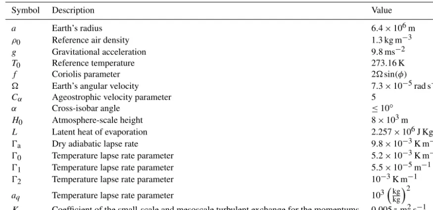
dry adiabatic lapse rate0a, latent heat of evaporationLand model parameters00, 01, 02, aq, T0are explained in Table 1.
Table 1.Atmosphere model parameters.
Symbol Description Value
a Earth’s radius 6.4×10⁶m
ρ0 Reference air density 1.3 kg m−3
g Gravitational acceleration 9.8 ms−2
T0 Reference temperature 273.16 K
f Coriolis parameter 2sin(φ)
Earth’s angular velocity 7.3×10⁻⁵rad s−1
Cα Ageostrophic velocity parameter 5
α Cross-isobar angle ≤10◦
H0 Atmosphere-scale height 8×10³m
L Latent heat of evaporation 2.257×10⁶J Kg−1
0a Dry adiabatic lapse rate 9.8×10⁻³K m−1
00 Temperature lapse rate parameter 5.2×10⁻³K m−1
01 Temperature lapse rate parameter 5.5×10⁻⁵m−1
02 Temperature lapse rate parameter 10−3K m−1
aq Temperature lapse rate parameter 103
kg
kg
2
Kz Coefficient of the small-scale and mesoscale turbulent exchange for the momentums 0.005zm2s−1
et al., 2013). The variableusfis the zonal surface wind; see Eq. (S10) in the Supplement.
The azonal component of the large-scale wind field de-scribes quasi-stationary planetary waves and depends on lat-itude, longitude and height. At the equivalent barotropic level (EBL), azonal geostrophic components of horizontal veloci-ties are computed by employing the definition of the stream functionψdepending on latitudeφand longitudeλ:
hu∗EBL(λ, φ)i = −1
a∇φhψ
∗
EBLi (5)
hvEBL∗ (λ, φ)i = 1
a∇λhψ
∗
EBLi, (6)
whereby the stream function can be subdivided into contri-butions from thermally and orographically induced waves depicted by subscripts “th” and “or”, respectively. They are considered to be additive due to linearity of the barotropic vorticity equations such that
hψEBL∗ i =90· hψth∗,EBLi + hψor∗,EBLi. (7) The parameter90is a tuning parameter which is necessary since smoothing is applied to dampen local moisture feed-backs in the model. This smoothing however reduces spatial gradients inψEBL∗ and thereforeu∗EBL andvEBL∗ themselves. The equation for the orographically induced waves is intro-duced in Sect. S1.2 in the Supplement.
The zeroth-order solution of the thermally induced waves of the barotropic vorticity equation is given by (see Sect. S1.3 in the Supplement)
hψth∗,0,EBLi = −hTEBL∗ i g
ρ0T02cosφ ∇φ
zEBL
Z
0
ρh[T (z)]idz. (8)
It is solved at two beta planes, for the Northern Hemisphere and Southern Hemisphere, respectively:
hψth∗,0,EBLiNH= − hTEBL∗ i g
ρ0T02cosβNH
∇φ
zEBL Z
0
ρh[T (z)]idz (9)
hψth∗,0,EBLiSH= − hTEBL∗ i g
ρ0T02cosβSH
∇φ
zEBL Z
0
ρh[T (z)]idz. (10)
The beta plane is an approximation in which the Coriolis pa-rameter is linearized to reference latitudesβNHandβSHfor the Northern Hemisphere and Southern Hemisphere, respec-tively. In the tropical belt, the variablehψth∗,0,EBLiis interpo-lated linearly between the two beta planes.
The standardized integrated heat content in Eq. (8)(Iv=
RzEBL
0 ρh[T (z)]idz)is calculated analytically by assuming a lapse rate0=00+01(Ta−T0) 1−aqqs2
−02ncsuch that T (z)=T (zEBL)−0 (z−zEBL). One obtains
Iv=ρ0([T (zEBL)]−[0]zEBL) H0
1−e−
zEBL H0
−0ρ0H0
(H0−zEBL)
e−
zEBL H0 −1
.
In addition,Ivis smoothed by five points in latitude to avoid
numerical artifacts which may arise due to spatial differenti-ating.
in-terpolation function. Planetary waves at other tropospheric levels are directly calculated from those at the EBL (see Sect. S1.1 in the Supplement).
Finally, the time-averaged kinetic energy of transient eddies hEk0i = 1
2
hu02i + hv02i is determined using the statistical–dynamical equations as described in Coumou et al. (2011). Since detailed derivations are provided in Coumou et al. (2011), we only briefly discuss the diagnostic equations for transient eddy activity here. The equations are derived starting from the equation of the kinetic energy of transient eddies:
∂hE0ki
∂t = −hVi · ∇hE
0 ki + hu
0V0i · ∇hui − hv0V0ii · ∇hvi+
Kfh1HhE0ki +Kfz1zhE0ki −KfshE 0 ki
+fhu0vag0 i − hv0u0agi. (11)
By assuming that the vertical (baroclinic) flux term is equipartitioned between the zonal and the meridional kinetic energy components, we can split Eq. (11) into three separate equations forhu02i,hv02iandhu0v0i:
∂hu02i
∂t = −hVi · ∇hu
02
i −2hu02i∂hui
∂x −2hu
0
v0i∂hui
∂y
+Ksyn
"
∂hui
∂z
2 +
∂hvi
∂z
2#
+Kfh1Hhu02i
+Kfz1zhu02i −Kfshu02i +f
hu0vag0 i − hv0u0agi
(12) ∂hv02i
∂t = −hVi · ∇hv
02
i −2hv02i∂hvi
∂y −2hv
02
i∂hvi
∂x
+Ksyn
" ∂hui
∂z
2 +
∂hvi
∂z
2#
+Kfh1Hhv02i
+Kfz1zhv02i −Kfshu02i +f
hu0vag0 i − hv0u0agi (13) ∂hu0v0i
∂t = −hVi · ∇hu
0
v0i − hu0Vi · ∇hvi − hv0Vi · ∇hui +Kfh1Hhu0v0i +Kfz1zhu0v0i −Kfshu0v0i
+fhv0v0agi − hu0u0agi. (14)
Here, Kfh and Kfz are internal atmospheric small-/mesoscale friction coefficients in the horizontal and vertical directions, respectively;Kfsis the surface friction coefficient; f is the Coriolis parameter; and the subscript “ag” denotes ageostrophic terms.
The terms forKsyn, the vertical macro-turbulent diffusion coefficient andfhv0vag0 i − hu0u0agi, need to be parameter-ized, which is derived in Coumou et al. (2011). This way, a set of diagnostic equations for synoptic transient eddies is derived which, as also seen in Eqs. (12)–(14), are all coupled to the large-scale wind field.
This provides us with a coupled set of equations for
hui,hvi,hu∗i,hv∗i,hu02i,hv02i and hu0v0i, which can be
solved. Cross terms likehu∗v∗ican be determined by
multi-plyinghu∗iwithhv∗iand taking the zonal mean of that quan-tity. All derivatives are determined numerically. The values of the parameters are listed in Table 1.
3 Forcing data and reanalysis data sets
The simulations were forced by multiyear averages of monthly mean climatological, El Niño and La Niña month data (surface temperature, surface specific humidity, temper-ature at 500 mb, geopotential height at 500 and 1000 mb) us-ing ERA-Interim reanalysis data (Dee et al., 2011) for 1983– 2009, as our aim is to show that Aeolus captures year-to-year variability associated with the ENSO cycle. We identi-fied 87 El Niño (74 La Niña) months using 3-month running means of Extended Reconstructed Sea Surface Temperature (ERSST) v4 anomalies (Huang et al., 2016) using the defini-tion that at least five consecutive overlapping seasons of sea surface temperature (SST) anomalies are greater than 0.5 K (less than−0.5 K) for El Niño (La Niña) events.
Multiyear averages of monthly mean, El Niño and La Niña month cumulative cloud fractions are taken from ISSCP (Rossow and Schiffer, 1999). The spatial resolution is 2.5×
2.5◦(lat×long) and the time range is 1983–2009.
We chose this time period, because the cumulative cloud fraction data, which are needed to calculate the lapse rate, are only available for this time period.
To avoid strong temperature gradients in the specified boundary conditions for the numerical experiments, we use the lapse rate equation to calculate temperatures at 1000 mb from those at 500 mb. We first calculate the lapse rate using the temperature field and specific humidity utilizing the equa-tion as given in Petoukhov et al. (2000) at 1000 mb. Then, we recalculate the temperature field at 1000 mb by employing the temperature field at 500 mb and the linear lapse rate equa-tion. This way, we ensure that the temperature at 500 mb is close to observations, and at the same time we have a vertical temperature realistic profile for a model like Aeolus. Since the ERA-Interim 500 mb temperatures contain an orographic component, we excludehψth∗,0,EBLiin Eq. (7) in order not to incorporate orographic forcing of planetary waves twice.
We optimized the parameters for the numerical solutions of the wind velocitiesu∗,v∗andhuias well as eddy kinetic energy hEk0i at 500 mb. To compare the strength and posi-tion of the Hadley and Ferrell cells between observaposi-tion and model, we calculate a zonal-mean mass fluxhmiin the lower troposphere using the zonal-mean meridional wind velocity
4 Model discretization
Aeolus operates on a reduced grid to overcome the restric-tion of small time steps near the poles due to the Courant– Friedrichs–Lewy (CFL) criteria (Jablonowski et al., 2009). In the grid generation, longitudinally adjacent cells are merged if their zonal width in meters would be less than half of the cell width at the Equator.
This way the reduced grid has the same resolution as a regular grid at the Equator, but at nominal resolution (3.75×
3.75◦) around the poles only six cells are defined. On the regular grid, the maximum permissible time step due to the CFL criteria would be approximately 5 min, while the limit for the reduced grid is approximately 2 h.
5 Calibration
Equations (1)–(14) are implemented in Aeolus and numeri-cally solved on a 3.75×3.75◦reduced grid with four tropo-spheric height levels (1000, 3000, 5000 and 9000 m).
The calibration of the winds is divided into two parts. First, we optimize the dynamical variables primarily driven by the thermal state of the atmosphere: the azonal velocities in zonal and meridional directionshu∗iandhv∗ias well as the zonal-mean zonal wind velocity hui. In the second step, we tune the zonal-mean synoptic kinetic energyhEk0iand the lower troposphere integrated mass flux hmi, which solely depend on the zonal-mean meridional windhvi.
A common approach for parameter tuning is simulated an-nealing (Ingber, 1996; Kirkpatrick, 1984). It is one experi-ment type in the multirun simulation environexperi-ment SimEnv for sensitivity and uncertainty analysis of model output (Flechsig et al., 2013) which we use for all calibration ex-periments. A schematic plot of the optimization process is shown in Sect. S3 in the Supplement.
For each model run, the thermal state of the atmosphere is kept constant (and initialized as described above) and the dynamical core is equilibrated to this thermal state. This typ-ically requires only a few time steps. Since we tune only the parameters of the dynamical core, Aeolus first calculates the clouds using its cloud scheme (Eliseev et al., 2013) to deter-mine the lapse rate and initialize the three-dimensional ther-mal state. After that, only the state of the dynamical core is updated each time step.
5.1 Dynamical core tuning – step 1
For a good starting point, the parameters are first tuned manually, providing “pre-optimized” values. Next, we define physically realistic parameter ranges for automatic tuning as listed in Table 2.
For the azonal wind velocities, we use a weighting func-tion which excludes the tropics (from 10◦S to 10◦N) and po-lar regions (poleward of 60◦S for the Southern Hemisphere to exclude influences of Antarctica and poleward of 70◦N for
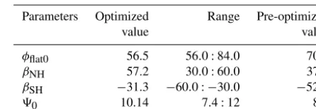
Table 2.Pre-optimized and optimized parameter sets and parameter ranges for optimization step 1.
Parameters Optimized Range Pre-optimized
value value
φflat0 56.5 56.0:84.0 70.0
βNH 57.2 30.0:60.0 37.5
βSH −31.3 −60.0: −30.0 −52.5
90 10.14 7.4:12 8.0
the Northern Hemisphere) such that the midlatitudes, where planetary waves are important, are optimized.
The non-excluded grid as well as the zonal-mean zonal wind are weighted byw (φ)= |cos(φ)|.
The total skill score for the scheme in step 1 is calculated by multiplying the individual skills for the azonal velocities in zonal and meridional directions(Su∗, Sv∗)and the skill for
the zonal-mean zonal wind velocity(Shui): S=Su∗Sv∗S
hui.
The goal of the optimization procedure is to maximize the skillS.
Skill score functions for individual variables are computed as in Taylor (2001):
S (φ, λ, t )= (1+rX)
4
(AX+1/AX)2
. (15)
In Eq. (15), rX is the coefficient of the spatial correlation
between the area-weighted modeled and observed fields of X; AX is the so-called relative spatial variation calculated
according to
AX=AX,M/AX,O. (16)
Here, the variable AX,M is the spatial average of
XM−XM,g
andXM,g is a globally averaged value of the modeled fieldXM. The observed field is similarly defined by AX,O.
5.2 Dynamical core tuning – step 2
For tuning the zonal-mean meridional wind velocityhvi, and in particular the strength and width of the Hadley cell, we use the vertical integral of the lower tropospheric integrated mass fluxhmi. In addition, we tune the zonal-mean area-weighted synoptic kinetic energyhEk0i. Both variables strongly depend on the dynamic fields tuned in step 1, which is the reason for tuning them in a separate second step.
Total skill score for the scheme in step 2 is calculated by multiplying the individual skills for the vertical integral of lower troposphere mass flux(Shmi)as well as the eddy ki-netic energy(ShE0
ki):
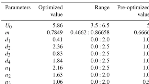
Table 3.Pre-optimized and optimized parameter sets and parameter ranges for optimization step 2.
Parameters Optimized Range Pre-optimized
value value
U0 5.86 3.5:6.5 5
m 0.7849 0.4662:0.86658 0.6666
d1 0.41 0.0:2.0 1.0
d2 2.36 0.0:2.5 1.0
d3 0.83 0.0:2.5 1.0
d4 1.84 0.0:2.5 1.0
n1 2.16 0.0:2.5 1.0
n2 1.63 0.0:2.0 1.0
n3 1.06 0.0:2.0 0.5
The goal of the optimization procedure is again to maxi-mize skillS.
The skill score function for the eddy kinetic energy is given by the Taylor skill score function (Eq. 15).
The skill score is then calculated by
Shmi= meanHadley_Obs−meanHadley_Model2rX2. (17) Here, rX is the coefficient of the spatial correlation
be-tween area-weighted modeled and observed fields (as in Eq. 15), meanHadley_Model and meanHadley_Obs are the mean values of the area-weighted modeled and observed mean mass flux. We use this more elaborate skill function to pro-mote a proper Hadley circulation in the model.
The weights of the lower troposphere mass flux hmi are calculated according to
w (φ)=
|cos(φ)| φ >60◦S 0 φ≤60◦S.
For calculating the mean intensity of the Hadley cell, we de-termine the roots of the mass flux in observation data close to 0 and 30◦which determine the Hadley cell latitudinal
bound-aries. This way, we have 36 values for the boundaries of the northern Hadley cell. Between these latitudinal borders, we calculate the mean strength of the Hadley cell.
In Table 3, the manually tuned (or pre-optimized) param-eters and their ranges are listed.
6 Results
6.1 Results of calibration – step 1
We compared the numerical solutions using the optimized parameters for the wind fieldshu∗i,hv∗iandhuiof climato-logical monthly averages, El Niño and La Niña months from ERA-Interim reanalysis (Dee et al., 2011) for 1983–2009.
The figures for azonal wind velocities are divided into six subplots. The left column shows observational data and the right column model data. The top row shows climatological
monthly averages, the middle row multiyear averages of El Niño months and the bottom row multiyear averages of La Niña months.
In Figs. 1 and 2, the azonal components of the zonal wind velocities (hu∗i)for February and August at 500 mb are dis-played, respectively. The figures show that with optimized parameters the model reasonably reproduces the main ob-served features both in terms of spatial position and magni-tude. In particular, the extratropical planetary waves are well captured with some minor discrepancies in the tropics. Both the seasonal cycle and the response to the ENSO cycle are well captured by the model.
Figures 3 and 4 show the same type of plots for the azonal meridional wind velocity (hv∗i). Also, for the meridional wind velocity, the most important features of the reanalysis data are well represented in the model. The model results coincide well in wind strength and spatial pattern with the reanalysis data. The wind strength in winter, for both clima-tological and El Niño months, is stronger than for La Niña months. In summer, the opposite is seen for both model and reanalysis data.
In Fig. 5, the zonal-mean zonal wind velocity (hui) at 500 mb is shown with the orange line representing reanaly-sis data, red representing model data with optimized param-eters and gray representing model data with pre-optimized parameters. The figure is subdivided into six subplots. The top row depictshuiin February and the bottom row shows
huiin August, while the columns show climatological data, El Niño data and La Niña data, respectively. It is noticeable that the results obtained with pre-optimized parameters are already reasonable. Apparently, the initial choice of tuning parameter values was already near the optimum, and hence the optimized parameters led only to small improvements of the model results. The Northern Hemisphere hui profile is well resolved in both seasons for both El Niño and La Niña months. Parameter optimization slightly improves the results in the tropics. The modeled amplitude ofhuiin the Southern Hemisphere is too small in February for all plots and too high in August.
The optimized parameters are listed in Table 2. TheβNH in the Northern Hemisphere has a higher value, whereas the βSHin the Southern Hemisphere has a lower value than the pre-optimized parameter values.
The last parameter is90and is changed to a higher value in order to strengthen speeds inhv∗iandhu∗i.
6.2 Results of calibration – step 2
We compared the numerical solutions using the optimized parameters for the zonal-mean lower troposphere integrated mass fluxhmiand eddy kinetic energyhE0ki
cal-ERA-Interim u*(500 mb) Aeolus u*(500 mb)
(a) (b)
Clim
-150 -100 -50 0 50 100 150
50 0
-50
-150 -100 -50 0 50 100 150
50 0
-50
(c) (d)
El
Niño
-150 -100 -50 0 50 100 150
50 0
-50
-150 -100 -50 0 50 100 150
50 0
-50
(e) (f)
La
Niña
-150 -100 -50 0 50 100 150
50 0
-50
-150 -100 -50 0 50 100 150
50 0
-50
u*(m s)
-10
-5
0 5 10 15 -1
Figure 1.Azonal large-scale zonal windu∗at 500 mb for all February months/El Niño February months/La Niña February months. The left column shows the results from reanalysis data and the right column shows the results from Aeolus received by optimized parameters. The model is forced by surface temperature, humidity and cumulus cloud fraction.
ERA-Interim u*(500 mb) Aeolus u*(500 mb)
(a) (b)
Clim
-150 -100 -50 0 50 100 150
50 0
-50
-150 -100 -50 0 50 100 150
50 0
-50
(c) (d)
El
Niño
-150 -100 -50 0 50 100 150
50 0
-50
-150 -100 -50 0 50 100 150
50 0
-50
(e) (f)
La
Niña
-150 -100 -50 0 50 100 150
50 0
-50
-150 -100 -50 0 50 100 150
50 0
-50
-10
-5
0 5 10
u*(m s-1)
ERA-Interim v*(500 mb) Aeolus v*(500 mb)
(a) (b)
Clim
-150 -100 -50 0 50 100 150
50 0
-50
-150 -100 -50 0 50 100 150
50 0
-50
(c) (d)
El
Niño
-150 -100 -50 0 50 100 150
50 0
-50
-150 -100 -50 0 50 100 150
50 0
-50
(e) (f)
La
Niña
-150 -100 -50 0 50 100 150
50 0
-50
-150 -100 -50 0 50 100 150
50 0
-50
v*
-5
0 5 10
(m s-1)
Figure 3.Azonal large-scale meridional wind velocityv∗at 500 mb for February (compare Fig. 1).
ERA-Interim v*(500 mb) Aeolus v*(500 mb)
(a) (b)
Clim
-150 -100 -50 0 50 100 150
50 0
-50
-150 -100 -50 0 50 100 150
50 0
-50
(c) (d)
El
Niño
-150 -100 -50 0 50 100 150
50 0
-50
-150 -100 -50 0 50 100 150
50 0
-50
(e) (f)
La
Niña
-150 -100 -50 0 50 100 150
50 0
-50
-150 -100 -50 0 50 100 150
50 0
-50
v*
-5
0 5 10
(m s-1)
Climatological(500 mb) El Niño(500 mb) La Niña(500 mb)
(a) (b) (c)
-50 0 50
-10
-5
0 5 10 15 20 25
〈
uFebruary
〉
(
m
s
-
)
-50 0 50
-10
-5
0 5 10 15 20 25
-50 0 50
-10
-5
0 5 10 15 20 25
(d) (e) (f)
-50 0 50
-10
-5
0 5 10 15 20 25
Latitude
〈
uAugust
〉
(
m
s
)
-50 0 50
-10
-5
0 5 10 15 20 25
Latitude
AeolusPRE-OPT AeolusOPT ERA-Int
-50 0 50
-10
-5
0 5 10 15 20 25
Latitude
-1
-1
Figure 5.Zonal-mean large-scale zonal wind velocityhu (z, φ)iat 500 mb. Panel(a)shows the climatological monthly mean zonal-mean zonal velocity in February,(b)the monthly mean zonal-mean velocity of El Niño February months and(c)the monthly mean zonal-mean velocity of La Niña February months. Panel(d) displays the monthly mean climatological zonal-mean zonal velocity in August,(e)the monthly mean zonal-mean velocity in El Niño August months and(f)the monthly mean zonal-mean velocity in La Niña August months. The yellow line represents zonal-mean large-scale zonal wind obtained by reanalysis data, the gray line is zonal-mean large-scale zonal wind velocity from Aeolus using pre-optimized parameters and the red line represents zonal-mean large-scale zonal wind velocity from Aeolus using optimized parameters.
ibration step 1. The ENSO cycle is clearly visible. However, the width of the Hadley cell (especially in August) is still too small compared to the width of the Hadley cell obtained by reanalysis data. The figure shows only plots with a latitudinal range from 60◦S to 90◦N as reanalysis data are spiky over Antarctica.
Figure 7 shows the zonal-mean eddy kinetic energyhEk0i. We show the same color code as in Fig. 6. Northern Hemi-sphere modeledhE0ki profile is again well resolved in both seasons and for El Niño and La Niña months with the pa-rameter optimization. Smaller spikes vanish such that the modeledhEk0ibetter matches the observed data. The param-eter optimization gained more improvement in the Northern Hemisphere (NH) than in the Southern Hemisphere (SH).
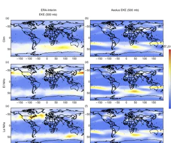
In Figs. 8 and 9, the eddy kinetic energieshEK0 ifor Febru-ary and August are displayed. The left column shows obser-vational data and the right column model data. The top row presents climatological monthly averages, the middle row El Niño months and the bottom row La Niña months.
The spatial position and the magnitude are well captured; seasons and the ENSO cycles are also well resolved, with some discrepancies in the tropics (i.e., the region over the Atlantic and Pacific oceans) and the Southern Hemisphere. In February and August, hEK0 i is stronger in the Northern Hemisphere than in the Southern Hemisphere for both the
climatology and in El Niño months. Only in La Niña months,
hEK0 iis weaker in the Northern Hemisphere.
The optimized parameters are listed in Table 3. The pa-rameters U0 andmfor optimizing the eddy kinetic energy are greater than the manually tuned values.
The parametersd3andn3are close to 1, whereas the pa-rametersd2, d4andn1are close to 2 and have a strong impact on the amplitude of the Hadley cell and the Ferrell cell. The parameter with the smallest influence isd1.
6.3 Comparison to CMIP5 models
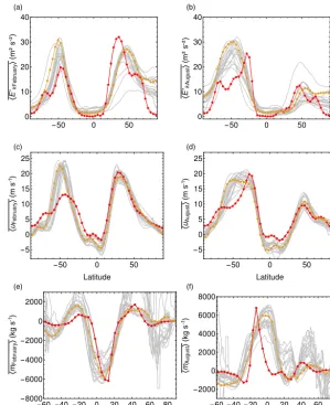
Figure 10 shows the comparison of February and August
hEk0i,hui andhmibetween CMIP5 models (gray lines), Ae-olus (red) and ERA-Interim data (orange). In general, CMIP5 models represent thehEk0i andhui very well in both hemi-spheres. However, in the Southern Hemisphere, the storm tracks, i.e.,hEk0i, of all models are too weak compared to ob-servations with Aeolus on the lower end of the CMIP5 range. Further, some individual CMIP5 models can have too-low or too-highhEk0iandhuicompared to ERA-Interim, similar to Aeolus.
ERA-Figure 6.Zonal-mean large-scale mass fluxhmi. Panel(a)shows the climatological monthly mean zonal-mean mass flux in February,(b)the monthly mean zonal-mean mass flux of El Niño February months and(c)the monthly mean zonal-mean mass flux of La Niña February months. Panel(d)displays the monthly mean climatological zonal-mean mass flux in August,(e)the monthly mean zonal-mean mass flux in El Niño August months and(f)the monthly mean zonal-mean mass flux in La Niña August months. The yellow line represents zonal-mean large-scale mass flux obtained by reanalysis data, the gray line is the zonal-mean large-scale mass flux from Aeolus using pre-optimized parameters and the red line represents the zonal-mean large-scale mass flux from Aeolus using optimized parameters.
Climatological(500 mb) El Niño(500 mb) La Niña(500 mb)
(a) (b) (c)
-50 0 50
0 10 20 30 40 50
Ek February
(m
²
s-²)
-50 0 50
0 10 20 30 40 50
-50 0 50
0 10 20 30 40 50
(d) (e) (f)
-50 0 50
0 10 20 30 40 50
Latitude
Ek August
(m
²
s-²)
-50 0 50
0 10 20 30 40 50
Latitude
AeolusPre-OPT AeolusOPT ERA-Int
-50 0 50
0 10 20 30 40 50
Latitude
ERA-Interim EKE (500 mb)
Aeolus EKE(500 mb)
(a) (b)
Clim
-150 -100 -50 0 50 100 150 50
0 -50
-150 -100 -50 0 50 100 150 50
0 -50
(c) (d)
El
Niño
-150 -100 -50 0 50 100 150 50
0 -50
-150 -100 -50 0 50 100 150 50
0 -50
(e) (f)
La
Niña
-150 -100 -50 0 50 100 150 50
0 -50
-150 -100 -50 0 50 100 150 50
0 -50
〈E'k〉(m 2
s2
)
0 20 40 60
-Figure 8.Eddy kinetic energyhEk0iin February at 500 mb (compare Fig. 1).
ERA-Interim EKE(500 mb)
Aeolus EKE(500 mb)
(a) (b)
Clim
-150 -100 -50 0 50 100 150 50
0 -50
-150 -100 -50 0 50 100 150 50
0 -50
(c) (d)
El
Niño
-150 -100 -50 0 50 100 150 50
0 -50
-150 -100 -50 0 50 100 150 50
0 -50
(e) (f)
La
Niña
-150 -100 -50 0 50 100 150 50
0 -50
-150 -100 -50 0 50 100 150 50
0 -50
0 20 40 60
〈E'k〉(m 2
s2
)
(a) (b)
-50 0 50
0 10 20 30 40
〈
E
'kFebruary
〉
(m
²
s
²)
-50 0 50
0 10 20 30 40
〈
E
'kAugust
〉
(m
²
s
²)
(c) (d)
-50 0 50
-5 0 5 10 15 20 25
Latitude
〈
uFebruary
〉
(m
s
)
-50 0 50
-5 0 5 10 15 20 25
Latitude
〈
uAugust
〉
(m
s
)
(e) (f)
-60 -40-20 0 20 40 60 80
-8000
-6000
-4000
-2000 0 2000
〈
mFebruary
〉
(k
g
s
)
-60-40-20 0 20 40 60 80
-2000 0 2000 4000 6000 8000
〈
mAugust
〉
(k
g
s
)
Latitude
--1
-1
-1
-1
Figure 10.Comparison to CMIP5 models. The orange line represents ERA-Interim data, the red line results from Aeolus and gray lines CMIP5 models (annual mean zonal-mean data).
Interim with some spiky behavior. Nevertheless, the width and strength of the Hadley cell is in most models well pre-sented, but the Ferrell cell is often too strong. Aeolus’ results give reasonable strength and width of the Ferrell cell, but the width of the Southern Hemisphere Hadley cell in August is too small compared to both reanalysis and CMIP5 models.
7 Summary and discussion
In this paper, we presented the atmosphere model Aeolus, which is a statistical–dynamical atmosphere model and be-longs to the class of intermediate complexity models. The equations of Aeolus are time averaged and the model has a spatial resolution of 3.75◦×3.75◦(lat×long). The three-dimensional structure of Aeolus is reconstructed using a set of two-dimensional, vertically averaged prognostic equations for temperature and water vapor (Petoukhov et al., 2000). The advantage of such types of models is the fast compu-tation time and for that reason the possibility to study and
simulate long time periods as well as conduct sensitivity ex-periments.
We performed parameter optimization of the dynamical core consisting of a large multidimensional parameter space and can be searched due to its fast computation time. For this approach, we used the simulated annealing optimiza-tion algorithm, which approximates the global minimum of a high-dimensional function. We divided the calibration into two parts. First, the azonal velocities in zonal and merid-ional directions as well as the zonal-mean zonal wind veloc-ity were optimized, because they are primarily driven by the thermal state of the atmosphere. In the second step, we opti-mized the zonal-mean synoptic kinetic energy and the lower troposphere integrated mass flux, and hence the zonal-mean meridional velocity, since those variables depend strongly on variables of step 1.
seasonal cycle as well as the ENSO cycle which is a prime goal of our model development efforts. Parameter optimiza-tion in particular improves representaoptimiza-tion of the Hadley cell in terms of strength and width.
In the Southern Hemisphere, the dynamical fields tend to be too weak. This model bias might be related to the miss-ing Antarctic ice sheet, upper tropospheric ozone, the con-stant lapse rate assumption or fundamental limitations of the equations. These possibilities will be analyzed in future work using the Potsdam Earth Model (POEM) to which Aeolus has been coupled.
Compared to CMIP5 models, Aeolus captures reasonably well the dynamical state of the atmosphere in the North-ern Hemisphere, particularly for monthly mean eddy kinetic energy hEk0i, zonal-mean wind velocity hui and mass flux
hmi. Especially the mass flux of the Ferrell cell is better captured than in other models, whereas the Southern Hemi-sphere Hadley cell width of Aeolus in August is too small compared to CMIP5 models.
Code and data availability. Code and data are stored in PIK’s long-term archive and are made available to interested parties on request.
Supplement. The supplement related to this article is available online at: https://doi.org/10.5194/gmd-11-665-2018-supplement.
Competing interests. The authors declare that they have no conflict of interest.
Acknowledgements. We thank ECMWF for making the ERA-Interim data available.
The work was supported by the German Federal Ministry of Ed-ucation and Research, grant no. 01LN1304A, (S.T., D.C.).
Alexey V. Eliseev’s contribution was partly supported by sup-ported by the Government of the Russian Federation (agreement no. 14.Z50.31.0033).
The authors gratefully acknowledge the European Regional Development Fund (ERDF), the German Federal Ministry of Edu-cation and Research and the Land Brandenburg for supporting this project by providing resources on the high-performance computer system at the Potsdam Institute for Climate Impact Research. Edited by: Didier Roche
Reviewed by: two anonymous referees
References
Berger, A., Fichefet, T., Gallée, H., Tricot, C., and van Ypersele, J. P.: Entering the glaciation with a 2-D coupled climate model, Quaternary Sci. Rev., 11, 481–493, https://doi.org/10.1016/0277-3791(92)90028-7, 1992.
Claussen, M., Mysak, L., Weaver, A., Crucifix, M., Fichefet, T., Loutre, M. F., Weber, S., Alcamo, J., Alexeev, V., Berger, A., Calov, R., Ganopolski, A., Goosse, H., Lohmann, G., Lunkeit, F., Mokhov, I., Petoukhov, V., Stone, P., and Wang, Z.: Earth sys-tem models of intermediate complexity: Closing the gap in the spectrum of climate system models, Clim. Dynam., 18, 579–586, https://doi.org/10.1007/s00382-001-0200-1, 2002.
Coumou, D., Petoukhov, V., and Eliseev, A. V.: Three-dimensional parameterizations of the synoptic scale kinetic energy and mo-mentum flux in the Earth’s atmosphere, Nonlin. Processes Geo-phys., 18, 807–827, https://doi.org/10.5194/npg-18-807-2011, 2011.
Dee, D. P., Uppala, S. M., Simmons, A. J., Berrisford, P., Poli, P., Kobayashi, S., Andrae, U., Balmaseda, M. A., Balsamo, G., Bauer, P., Bechtold, P., Beljaars, A. C. M., van de Berg, L., Bid-lot, J., Bormann, N., Delsol, C., Dragani, R., Fuentes, M., Geer, A. J., Haimberger, L., Healy, S. B., Hersbach, H., Hólm, E. V., Isaksen, L., Kållberg, P., Köhler, M., Matricardi, M., Mcnally, A. P., Monge-Sanz, B. M., Morcrette, J. J., Park, B. K., Peubey, C., de Rosnay, P., Tavolato, C., Thépaut, J. N., and Vitart, F.: The ERA-Interim reanalysis: Configuration and performance of the data assimilation system, Q. J. Roy. Meteor. Soc., 137, 553–597, https://doi.org/10.1002/qj.828, 2011.
Dobrovolski, S. G.: Stochastic Climate Theory, Springer-Verlag Berlin Heidelberg, 2000.
Ehlers, E. and Krafft, T.: Understanding the Earth System: Com-partments, Processes and Interactions, Springer-Verlag, Berlin, Heidelberg, 2001.
Eliseev, A. V., Coumou, D., Chernokulsky, A. V., Petoukhov, V., and Petri, S.: Scheme for calculation of multi-layer cloudiness and precipitation for climate models of intermediate complexity, Geosci. Model Dev., 6, 1745–1765, https://doi.org/10.5194/gmd-6-1745-2013, 2013.
Eliseev, A. V., Mokhov, I. I., and Chernokulsky, A. V.: An en-semble approach to simulate CO2emissions from natural fires,
Biogeosciences, 11, 3205–3223, https://doi.org/10.5194/bg-11-3205-2014, 2014a.
Eliseev, A. V., Demchenko, P. F., Arzhanov, M. M., and Mokhov, I. I.: Transient hysteresis of near-surface permafrost response to external forcing, Clim. Dynam., 42, 1203–1215, https://doi.org/10.1007/s00382-013-1672-5, 2014b.
Flechsig, M., Böhm, U., Nocke, T., and Rachimow, C.: The Multi-Run Simulation Environment SimEnv, available at: https://www.pik-potsdam.de/research/ transdisciplinary-concepts-and-methods/tools/simenv/ (last access: 26 January 2018), 2013.
Fraedrich, K. and Böttger, H.: A Wavenumber-Frequency Analysis of the 500 mb Geopotential at 50◦N, J. At-mos. Sci., 35, 745–750, https://doi.org/10.1175/1520-0469(1978)035<0745:AWFAOT>2.0.CO;2, 1978.
Part II: Model sensitivity, Clim. Dynam., 17, 735–751, https://doi.org/10.1007/s003820000144, 2001.
Harvey, L. D. D.: Milankovitch Forcing, Vegetation Feedback, and North Atlantic Deep-Water Formation, J. Climate, 2, 800–815, 1989.
Holland, M., Bitz, C., Eby, M., and Weaver, A.: The Role of Ice – Ocean Interactions in the Variabil-ity of the North Atlantic Thermohaline Circulation, J. Climate, 14, 656–675, https://doi.org/10.1175/1520-0442(2001)014<0656:TROIOI>2.0.CO;2, 2001.
Huang, B., Thorne, P. W., Smith, T. M., Liu, W., Lawrimore, J., Banzon, V. F., Zhang, H.-M., Peterson, T. C., and Menne, M.: Further Exploring and Quantifying Uncertainties for Extended Reconstructed Sea Surface Temperature (ERSST) Version 4 (v4), J. Climate, 29, 3119–3142, https://doi.org/10.1175/JCLI-D-15-0430.1, 2016.
Imkeller, P. and von Storch, J.-S.: Stochastic Climate Models, Birkhäuser, 2012.
Ingber, L.: Adaptive simulated annealing (ASA): Lessons learned, Control Cybern., 25, 32–54, 1996.
Jablonowski, C., Oehmke, R. C., and Stout, Q. F.: Block-structured adaptive meshes and reduced grids for atmospheric general circulation models, Philos. T. Roy. Soc. A, 367, 4497–522, https://doi.org/10.1098/rsta.2009.0150, 2009.
Kirkpatrick, S.: Optimization by simulated annealing: Quantitative studies, J. Stat. Phys., 34, 975–986, https://doi.org/10.1007/BF01009452, 1984.
Knutti, R., Stocker, T. F., Joos, F., and Plattner, G.-K.: Constraints on radiative forcing and future climate change from obser-vations and climate model ensembles, Nature, 416, 719–723, https://doi.org/10.1038/416719a, 2002.
Latif, M.: Dynamics of interdecadal variability in coupled ocean-atmosphere models, J. Cli-mate, 11, 602–624, https://doi.org/10.1175/1520-0442(1998)011<0602:DOIVIC>2.0.CO;2, 1998.
McGuffie, K. and Henderson-Sellers, A.: A Climate Modelling Primer, 3rd Edn., J. Wiley and Sons, 2005.
Montoya, M., Griesel, A., Levermann, A., Mignot, J., Hofmann, M., Ganopolski, A., and Rahmstorf, S.: The earth system model of intermediate complexity CLIMBER-3alpha. Part I: Description and performance for present-day conditions, Clim. Dynam., 25, 237–263, https://doi.org/10.1007/s00382-005-0044-1, 2005. Petoukhov, V., Ganopolski, A., Brovkin, V., Claussen, M., Eliseev,
A. V., Kubatzki, C., and Rahmstorf, S.: CLIMBER 2: a climate system model of intermediate complexity. Part I: model descrip-tion and performance for present climate, Clim. Dynam., 16, 1– 17, https://doi.org/10.1007/PL00007919, 2000.
Polyakov, I. V., Alekseev, G. V., Bekryaev, R. V., Bhatt, U. S., Colony, R., Johnson, M. A., Karklin, V. P., Walsh, D., and Yulin, A. V.: Long-term ice variability in Arctic marginal seas, J. Climate, 16, 2078–2085, https://doi.org/10.1175/1520-0442(2003)016<2078:LIVIAM>2.0.CO;2, 2003.
Rossow, W. B. and Schiffer, R. A.: Advances in Un-derstandig Clouds from ISCCP, B. Am. Meteorol. Soc., 80, 2261–2287, https://doi.org/10.1175/1520-0477(1999)080<2261:AIUCFI>2.0.CO;2, 1999.
Saltzman, B.: A Survey of Statistical-Dynamical Models of the Terrestrial Climate, Adv. Geophys., 20, 183–304, https://doi.org/10.1016/S0065-2687(08)60324-6, 1978. Schmittner, A. and Stocker, T. F.: The stability of the
ther-mohaline circulation in global warming experiments, J. Climate, 12, 1117–1133, https://doi.org/10.1175/1520-0442(1999)012<1117:TSOTTC>2.0.CO;2, 1999.
Taylor, K. E.: Summarizing multiple aspects of model perfor-mance in a Single Diagram, J. Geophys. Res., 106, 7183–7192, https://doi.org/10.1029/2000JD900719, 2001.