Parameterizing microphysical effects on variances and covariances of moisture and heat content using a multivariate probability density function: a study with CLUBB (tag MVCS)

(1)

www.geosci-model-dev.net/9/4273/2016/ doi:10.5194/gmd-9-4273-2016

Parameterizing microphysical effects on variances and covariances

of moisture and heat content using a multivariate probability

density function: a study with CLUBB (tag MVCS)

Brian M. Griffin and Vincent E. Larson

University of Wisconsin – Milwaukee, Department of Mathematical Sciences, Milwaukee, WI, USA Correspondence to:Brian M. Griffin ([email protected])

Received: 5 May 2016 – Published in Geosci. Model Dev. Discuss.: 2 June 2016 Revised: 29 August 2016 – Accepted: 7 October 2016 – Published: 25 November 2016

Abstract. Microphysical processes, such as the formation, growth, and evaporation of precipitation, interact with vari-ability and covariances (e.g., fluxes) in moisture and heat content. For instance, evaporation of rain may produce cold pools, which in turn may trigger fresh convection and pre-cipitation. These effects are usually omitted or else crudely parameterized at subgrid scales in weather and climate mod-els.

A more formal approach is pursued here, based on predictive, horizontally averaged equations for the vari-ances, covarivari-ances, and fluxes of moisture and heat content. These higher-order moment equations contain microphysical source terms. The microphysics terms can be integrated an-alytically, given a suitably simple warm-rain microphysics scheme and an approximate assumption about the multi-variate distribution of cloud-related and precipitation-related variables. Performing the integrations provides exact expres-sions within an idealized context.

A large-eddy simulation (LES) of a shallow precipitat-ing cumulus case is performed here, and it indicates that the microphysical effects on (co)variances and fluxes can be large. In some budgets and altitude ranges, they are dominant terms. The analytic expressions for the integrals are imple-mented in a single-column, higher-order closure model. In-teractive single-column simulations agree qualitatively with the LES. The analytic integrations form a parameterization of microphysical effects in their own right, and they also serve as benchmark solutions that can be compared to non-analytic integration methods.

1 Introduction

(2)

and/or exhibit mesoscale organization (e.g., Rauber et al., 2007; Xue et al., 2008).

Some effects of microphysics influence the spatial ar-rangement of cloud parcels. For instance, precipitation may lead to an increase in cloud diameter or to the development of mesoscale cloud organization (e.g., Kuang and Brether-ton, 2006; Khairoutdinov and Randall, 2006; Schlemmer and Hohenegger, 2014). Such effects of microphysics on cloud structure will not be discussed here. Instead, the focus will be on the effects of microphysics on thevariances and co-variancesof cloud-related fields. Microphysics affects more than just horizontal averages; it also affects variability. For instance, rain production in the moistest parts of a cloud tends to diminish variability in cloud water. Also, evapora-tive cooling of rain in cold downdrafts below cloud base may increase the variability in temperature in the subcloud layer. Even though the effects of microphysics on cloudstructure may be difficult to quantify, the effects of microphysics on variances and covariances are simpler to define and calcu-late. Those effects appear as well-defined covariance terms on the right-hand side of spatially filtered equations for the scalar variances and turbulent fluxes. These filtered moment equations can be derived rigorously from the governing equa-tions, and the microphysical terms emerge naturally from the derivation. However, most coarse-resolution climate or weather models either treat such effects phenomenologically (e.g., Grandpeix and Lafore, 2010; Rio et al., 2013; Bechtold et al., 2014) or else ignore them entirely.

The microphysical terms in the predictive variance and covariance equations can be parameterized by integrating microphysical formulas over the probability density func-tion (PDF) representing subgrid variability. A primary pur-pose of this paper is to perform those integrals analytically and to implement the resulting formulas in a particular PDF parameterization, the Cloud Layers Unified By Binormals (CLUBB) model. The needed integrals are set up in Ap-pendix A and are solved by the expressions given in the Supplement. The integrals can be performed analytically be-cause the microphysical formulas that are integrated are sim-ple power laws (Khairoutdinov and Kogan, 2000), and be-cause it is assumed that the variables involved are distributed according to a multivariate PDF based on normal and lognor-mal functions (Griffin and Larson, 2016). The analytic solu-tions to the integrals are used directly as a parameterization. Alternatively, the implementation of the integrals may also serve as a benchmark calculation that is based on idealized (Khairoutdinov–Kogan) microphysics. The benchmark cal-culation can be used to assess the accuracy and convergence of more general integration methods, as done in Larson and Schanen (2013). Full evaluation of the use of the integrals as a parameterization is deferred to future work, but for il-lustrative purposes, single-column CLUBB simulations of a shallow convective case, Rain in Cumulus Over the Ocean (RICO) (van Zanten et al., 2011), and a marine stratocumu-lus case are presented. Budgets from a large-eddy simulation

(LES) model are also presented. The LES indicates which variances and covariances are most influenced by microphys-ical processes. In addition, the LES provides a benchmark budget of each covariance. Each budget term from LES cor-responds to a budget term in CLUBB, allowing for a close, term-by-term comparison of model processes. This sort of detailed comparison is infeasible with more phenomenolog-ical parameterizations.

To clarify, we note that the microphysical terms we study here are the ones that appear in the variance and covariance equations, not the grid mean equations. Microphysical effects on the grid means have been studied in several prior works (e.g., Zhang et al., 2002; Larson and Griffin, 2006, 2013; Morrison and Gettelman, 2008; Cheng and Xu, 2009; Griffin and Larson, 2013; Boutle et al., 2014). The microphysical ef-fects on the grid means can shift the subgrid PDF to smaller or larger values, but, unlike the covariance terms, they can-not directly change the shape of the PDF. The microphysical covariance terms are important because (1) they damp vari-ability (i.e., narrow the PDF) via the effects of precipitation rather than turbulence; and (2) they generate variability (i.e., widen the PDF) below cloud via the effects of rain evapora-tion.

The remainder of the paper is organized as follows. Sec-tion 2 overviews the origin of the microphysical terms from the predictive equations, summarizes the microphysics scheme involved in the development of this parameterization, and summarizes the multivariate PDF used by CLUBB. Sec-tion 3 describes the test case simulaSec-tions, the LES used for comparison, and the setup of the CLUBB model. Section 4 compares the budget terms for relevant variances and covari-ances between the LES and CLUBB. Section 5 contains con-cluding remarks.

2 Mathematical and physical overview

This section indicates where the microphysical terms enter CLUBB’s equation set. Microphysical terms have appeared in versions of CLUBB’s grid-mean equations for some years, but now microphysics terms also appear in CLUBB’s predic-tive equations for scalar variances and covariances.

CLUBB is a single-column model (SCM) that predicts variances and covariances involving vertical velocity, mois-ture, and temperature fields using spatially filtered moment equations (Golaz et al., 2002; Larson and Golaz, 2005; Lar-son and Griffin, 2013; Griffin and LarLar-son, 2013). CLUBB uses a multivariate PDF to represent subgrid variability in vertical velocity, moisture, temperature, and hydrometeor fields. The subgrid PDF is used to close the higher-order mo-ment terms found in the predictive momo-ment equations and also to provide information on cloud water and cloud frac-tion.

(3)

and liquid water potential temperature,θl. Total water mixing ratio is defined such thatrt=rv+rc, whererv is water va-por mixing ratio andrcis (liquid) cloud water mixing ratio. Liquid water potential temperature is defined by the equation

θl=Tl

_p

p0 −_CRd

pd

, (1)

wherepis pressure,p0is a reference pressure of 1.0×105Pa,

Rdis the gas constant for dry air, andCpdis the specific heat of dry air at a constant pressure. Liquid water temperature,

Tl, is defined as

Tl=T− Lv

Cpdrc, (2)

whereT is temperature and Lv is the latent heat of

vapor-ization. In subsaturated air,rtreduces torvandθlreduces to

potential temperature,θ.

The CLUBB model usesrtandθlbecause those variables

are conserved with regard to adiabatic processes and phase changes between water vapor and liquid cloud water. How-ever,rtandθlare not conserved with respect to transfers be-tween precipitation and water vapor or cloud water. As a re-sult, the time-tendency equations for each ofrtandθlinclude a microphysics tendency term. Omitting all other terms, such as advection, these equations can be written as

∂rt

∂t =. . .+ ∂rt

∂t _mc

,and (3)

∂θl

∂t =. . .+ ∂θl

∂t

mc

; (4)

wheret is time, and where ∂rt

∂t _mcand

∂θl

∂t

_mcare the

micro-physics tendency terms forrt andθl, respectively. They are the source or sink of rt andθl due to microphysics process rates.

The time-tendency equations are split into mean and turbu-lent components. For the remainder of this paper, an overbar will denote a mean value, while the prime symbol 0will do-nate a deviation from the mean value (turbulent value). The Reynolds-averaged predictive equations for grid-box mean fieldsrtandθlinclude the terms

∂rt

∂t =. . .+ ∂rt

∂t _mc

,and (5)

∂θl

∂t =. . .+ ∂θl

∂t _mc

. (6)

The omitted terms in the predictive equations forrtandθlare

listed in Golaz et al. (2002), with the only change being that the CLUBB equation set is now written in anelastic form.

In order to obtain the fields necessary to generate the PDF, CLUBB also contains predictive equations for the subgrid

variances and covariances involvingw,rt, andθl. The fields that contain a microphysics term arew0_r0

t,w0θl0,rt02,θl02, and r_t0θ_l0. The Reynolds-averaged predictive equations for these subgrid variances and covariances include the terms:

∂w0_r0 t

∂t =. . .+w 0∂rt

∂t 0

mc

, (7)

∂w0_θ0 l

∂t =. . .+w 0∂θl

∂t 0

mc

, (8)

∂r_t02

∂t =. . .+2r 0 t

∂rt ∂t

0

mc

, (9)

∂θ_l02

∂t =. . .+2θ 0 l

∂θl ∂t

0

mc

,and (10)

∂r_t0θ_l0

∂t =. . .+ r 0 t

∂θl ∂t

0

mc

+ θ_l0∂rt ∂t

0

mc

. (11)

The full forms, including all omitted terms, of the predic-tive equations forw0_r0

t,w0θl0,r 02

t ,θl02, andr 0

tθl0 are given by

Eqs. (26), (27), (28), (29), and (30), respectively, in Sect. 4. Ifrtandθlwere extended to include precipitation, the

ex-tended variables would be conserved with respect to transfers between hydrometeors and water vapor or cloud water (mi-crophysics process rates). This is a simplification, but we do not choose to extend the variables to include precipitation because it would lead to a complication. Namely, it would cause the microphysical effects to appear in sedimentation terms, and the sedimentation terms contain vertical deriva-tives, unlike the process rate terms. Furthermore, some turbu-lent components of the sedimentation term contain a vertical derivative within a horizontal average. To illustrate, consider a hydrometeor-inclusive total water mixing ratio, denotedrT, such thatrT=rv+rc+rr, whererris rainwater mixing ratio. For simplicity,rrwill be the only hydrometeor considered in the microphysics. The microphysics term on the right-hand side of the Reynolds-averagedr_T02predictive equation would have the form

2r_T0

−1

ρs

∂ρsVrrrr

∂z 0

=

− 2

ρs

r_T0 ∂ρsVrrr 0 r

∂z −

2

ρs

r_T0 ∂ρsV 0 rrrr

∂z −

2

ρs

r_T0 ∂ρsV 0 rrr

0 r

∂z ,

where Vrr is the sedimentation velocity of rr, ρs is the dry, base-state air density, and z is height. Every predic-tive moisture or temperature (co)variance equation would contain terms analogous to the above sedimentation terms. Since these terms contain vertical derivatives (∂/∂z) embed-ded within integrals over the horizontal, they are difficult to treat analytically and cannot be described solely by a mul-tivariate subgrid PDF at a single vertical grid level. For this reason, CLUBB’s calculations of the microphysics terms use

(4)

2.1 Khairoutdinov–Kogan microphysics

The preceding section describes where microphysical ten-dencies, of any kind, enter CLUBB’s equation set. This sec-tion describes how the microphysical tendencies are related to the specific processes of autoconversion, accretion, and evaporation.

The source terms for the model predictive equations require microphysical process rates from a microphysics scheme. The scheme used here is the warm microphysics scheme described in Khairoutdinov and Kogan (2000, here-after KK). KK is a two-moment scheme that predictsrrand rain drop concentration (per unit mass),Nr. It was developed by using the least squares method to find a “best-fit” curve through microphysical rate data that were generated by sim-ulating a drizzling stratocumulus case using an explicit (or “bin”) microphysics scheme.

The KK scheme was chosen because of its simplicity. It expresses microphysical rates as power laws of two or three variables, which means that the product of a microphysical rate and the corresponding PDF is always integrable. More recently, the coefficients and exponents in the KK scheme have been tailored to cumulus clouds (Kogan, 2013). The Ko-gan scheme is covered by the analytic integrals presented in this paper because they are generalized for arbitrary coeffi-cients and exponents. However, this paper uses the original KK coefficients and exponents because the KK scheme has been widely used for a variety of cloud types and is adequate for our idealized purposes.

The KK warm microphysics scheme producesrrthrough the processes of autoconversion (collision) and accretion (collection). These processes produce rainwater, deplete cloud water, and leave water vapor unchanged. As a result, these processes increase the value ofθl, as shown by Eqs. (1)

and (2), and decrease the value ofrt. Evaporation reducesrr

as rain falls through subsaturated air. Condensational growth does not apply to rainwater in CLUBB. Instead, all supersat-uration is automatically applied to cloud water. When rain-water evaporates, cloud rain-water remains unchanged, andrt

in-creases due to the increase in water vapor. Meanwhile, evap-orative cooling decreasesθl due to the decrease in

tempera-ture.

The relationship of all three KK microphysics tendencies to thertmicrophysics tendency can be written as

∂rt ∂t _mc

= −∂rr

∂t _auto − ∂rr ∂t _accr − ∂rr ∂t _evap , (12)

where ∂rr

∂t

autois the rate of change ofrrdue to the process

of autoconversion, ∂rr

∂t

accris the rate of change ofrrdue to

the process of accretion, and ∂rr

∂t

_evapis the rate of change of rrdue to the process of evaporation. Note that when evapo-ration occurs, ∂rr

∂t

_evap<0. The relationship of all three

ten-dencies toθlmicrophysics tendency can be written as

∂θl ∂t _mc = Lv Cpd _p p0 −Rd

C_pd _∂r

r ∂t auto

+∂rr

∂t accr

+ ∂rr

∂t evap ! . (13)

The decrease in temperature from the evaporation of a unit of rainwater is the same as the decrease in temperature from the evaporation of the same amount of cloud water.

The Reynolds-averaged microphysics term in the predic-tive equation forw0_r0

t, as found in Eq. (7), is rewritten as w0∂rt

∂t 0 mc

= −w0∂rr

∂t 0 auto

−w0∂rr

∂t 0 accr

−w0∂rr

∂t 0 evap . (14)

Likewise, the Reynolds-averaged microphysics term in the predictive equation forw0_θ0

l, as found in Eq. (8), is rewritten

as

w0∂θl ∂t 0 mc = Lv Cpd _p p0 − R_d C_pd

× w0∂rr

∂t 0 auto

+ w0∂rr

∂t 0 accr

+ w0∂rr

∂t 0 evap ! . (15)

Any variability ofp within the grid box is ignored for sim-plicity. Additionally, the −Rd/Cpd exponent would greatly limit the effects of variability ofpon the solution. As a re-sult,pis used in the equation. In the predictive equation for

r_t02, Eq. (9), the microphysics term becomes

r_t0∂rt ∂t 0 mc

= −r_t0∂rr

∂t 0 auto

−r_t0∂rr ∂t 0 accr

−r_t0∂rr ∂t 0 evap . (16)

In the predictive equation forθ_l02, Eq. (10), the microphysics term becomes

θ_l0∂θl ∂t 0 mc = Lv Cpd _p p0 −_CRd

pd

× θ_l0∂rr

∂t 0 auto

+θ_l0∂rr ∂t 0 accr

+θ_l0∂rr ∂t 0 evap ! . (17)

The Reynolds-averaged microphysics terms in the predictive equation forr_t0θ_l0, as found in Eq. (11), are rewritten as

θ_l0∂rt ∂t 0 mc =

−θ_l0∂rr

∂t 0 auto

− θ_l0∂rr

∂t 0 accr

− θ_l0∂rr

∂t 0 evap

(5)

r_t0∂θl ∂t

0

mc

= Lv

Cpd

p p0

−Rd Cpd

× r_t0∂rr

∂t 0

auto

+ r_t0∂rr

∂t 0

accr

+ r_t0∂rr

∂t 0

evap !

. (19)

The above equation set contains nine individual microphysi-cal covariance terms, each involving one ofw,rt, orθlwith

one of autoconversion, accretion, or evaporation rate. These terms can be parameterized through use of the PDF method. 2.2 PDF method

The multivariate PDF used by CLUBB consists ofw,rt,θl,

all hydrometeor species used by the selected microphysics scheme (in the case of KK microphysics,rrandNr), and an extended cloud droplet concentration, Ncn, which is equal to cloud droplet concentration, Nc, within cloud, but has a positive value outside of cloud (Griffin and Larson, 2016). CLUBB’s PDF is a weighted mixture, or sum, of two multi-variate normal/lognormal functions. Each multimulti-variate func-tion is known as a PDF component.

When variables are integrated out of the multivariate PDF, a marginal PDF consisting of fewer variables remains. When all variables but one are integrated out of the PDF, the result is a univariate marginal or individual marginal. The individ-ual marginal for each of w,rt, andθl is a two-component

normal (also known as a binormal) distribution. The two-component shape allows skewness to be included in model fields. The individual marginal for Ncn is assumed to be a

(single) lognormal distribution.

The individual marginal for each of rr and Nr is delta-lognormalwithin each PDF component(Griffin and Larson, 2016). Each PDF component can contain precipitating and precipitationless regions. The fraction of each PDF compo-nent that contains any hydrometeor species (other than cloud liquid water) is known as the component’s precipitation frac-tion. The precipitationless region is represented by a delta at 0 for all hydrometeor species. Within precipitation, a lognor-mal distribution is used to represent a hydrometeor species. The lognormal distributions can differ between the two com-ponents, so that when the components are summed to form the overall distribution, a delta double lognormal (DDL) dis-tribution results.

The PDF method for parameterizing the nine microphysics covariance terms requires analytic integration over the multi-variate PDF. As listed in Griffin and Larson (2016), the gen-eral form of a multivariate PDF ofncomponents andD vari-ables, whereDcan be all the variables involved in the PDF or any subset of those, is given by

P (x1, x2, . . ., xD)= n X

i=1

ξ(i)P(i)(x1, x2, . . ., xD) , (20)

whereξ(i)is the mixture fraction, or relative weight of theith

PDF component. The sum of the mixture fractions is equal to 1.

TheDvariables listed are categorized, and the firstJ vari-ables are normally distributed in each PDF component (w,

rt, andθl), the nextK variables are lognormally distributed

(Ncn), and the lastvariables are the hydrometeor species

that are distributed delta-lognormally in each PDF compo-nent (rrand/orNr). The equation for theith PDF component

is

P(i)(x1, x2, . . ., xD)=

fp(i)P(J,K+)(i)(x1, x2, . . ., xD)

+ 1−fp(i)

P(J,K)(i)(x1, x2, . . ., xJ+K) D

Y

=J+K+1 δ (x)

!

,

(21) wherefp(i)is the precipitation fraction in theith PDF

com-ponent. The subscripts in the ith component, P(J,K)(i) or P(J,K+)(i), denote the number of normal variates,J, and the

number of lognormal variates,KorK+, used in Eq. (22). Both the precipitating and precipitationless portions (sub-components) of Eq. (21) contain a hybrid normal/lognormal distribution of mvariables, where the first j variables are normally distributed and the remainingkvariables are log-normally distributed. The general form of this multivariate normal/lognormal PDF is given by (Fletcher and Zupanski, 2006)

P(j,k)(i)(x1, x2, . . ., xm)=

1

(2π )m26(i)

1 2

m Y

τ=j+1

1

xτ !

×exp

−1

2 x−µ(i)

T

6−1_(i) x−µ_(i)

, (22)

wherexis anm×1 vector of the variables (in normal space) in the PDF andµ_(i)is anm×1 vector of the (normal-space) PDF subcomponent means. The transpose of the vector is denoted T. Them×m(normal-space) covariance matrix is denoted6_(i)and its determinant is denoted6_(i)

(Fletcher

and Zupanski, 2006).

(6)

Also useful for gaining intuition are the bivariate marginals listed in Sect. S3 of the Supplement. A normal– normal bivariate form is listed in Eq. (S4), a lognormal– lognormal form is listed in Eq. (S6), and a hybrid normal– lognormal form is listed in Eq. (S5). Where a lognormal variate appears, the corresponding axis takes on only non-negative values and has a long tail. Which bivariate form is used depends on which functional forms are used to represent the variates of interest, e.g., rainwater mixing ratio (lognor-mal) or vertical velocity (nor(lognor-mal).

Using a two-component PDF requires a method to divide oneoverall(grid-box) mean value of a variable into two PDF componentmean values of that variable. Likewise, one over-all variance needs to be split into two PDF component stan-dard deviations. The multivariate PDF also requires informa-tion on the correlainforma-tions between variables.

The PDF component means, standard deviations, and cor-relations involvingw,rt, andθl, as well as the mixture frac-tions, are calculated according to the Analytic Double Gaus-sian 1 (ADG1) PDF presented in Sect. (d) of the Appendix of Larson et al. (2002). The overall (grid-box) precipita-tion fracprecipita-tion is set to the maximum cloud fracprecipita-tion found at or above that grid level (Morrison and Gettelman, 2008). The calculation of the component precipitation fractionsfp(i)

from the overall precipitation fraction are outlined in Griffin and Larson (2016). Also described there is the calculation of the PDF component means and standard deviations involving

Ncn,rr, andNr. Interactive CLUBB runs prescribe a constant ratio of the precipitation variance to the square of the in-precipitation mean forrrandNr. Additionally, all remaining correlations between variables are prescribed constants.

The covariance of PDF variablesx1andx2can be calcu-lated by

x₁0x₂0 =

Z Z

(x1−x1) (x2−x2) P (x1, x2)dx2dx1. (23) The covariance of a PDF variable and a microphysics func-tion (written in terms of PDF variables) can be calculated in the same manner. For example, the covariance ofθland KK evaporation rate found in Eqs. (17) and (18) can be rewritten as

θ_l0∂rr ∂t

0

evap

=

θl−θl

_∂r

r ∂t

evap

− ∂rr

∂t

evap !

, (24)

where mean evaporation rate, ∂rr

∂t

_evap, is also calculated by

integrating over the PDF (Supplement to Griffin and Larson, 2016; Larson and Griffin, 2013). The KK evaporation rate can be written as a function ofθl,rt,rr, andNr, so here it will be referred to as EV(θl, rt, rr, Nr). The covariance ofθland KK evaporation rate is calculated by

θ_l0∂rr ∂t

0

evap

=

Z Z Z Z

θl−θl EV(θl, rt, rr, Nr)−EV(θl, rt, rr, Nr)

×P (θl, rt, rr, Nr)dNrdrrdrtdθl. (25)

The remaining eight covariances involving microphysical functions are calculated in the same manner. Further and more detailed description of this method can be found in Ap-pendix A and the Supplement.

3 Test case and model setups

To perform an initial test of the parameterization, we choose the Rain in Cumulus Over the Ocean (RICO) model inter-comparison case of a precipitating shallow cumulus layer (van Zanten et al., 2011). The intercomparison model con-figuration is based on a field study conducted off the coast of Antigua and Barbuda (Rauber et al., 2007). RICO uses pre-scribed radiative and large-scale forcings for temperature and moisture, as well as prescribed large-scale subsidence. These quantities vary with altitude but are constant over time. The surface fluxes are calculated using bulk aerodynamic equa-tions. The simulation was run for a period of 72 h.

RICO was chosen as a test case for two main reasons. First, ice microphysics is not necessary for a shallow trade-wind cumulus case; hence, a warm microphysics scheme is sufficient. Secondly, RICO is a partly cloudy case that pre-cipitates over a small portion of the horizontal domain and contains significant variance ofrrwithin the precipitating re-gion. These factors lead to significant microphysical effects on the subgrid variances and covariances.

In order to demonstrate that the effects of microphysics on the same subgrid variances and covariances are negligible in a stratocumulus test case, we also ran the drizzling stra-tocumulus test case based on research flight two (RF02) of the second Dynamics and Chemistry of Marine Stratocumu-lus (DYCOMS-II) field study (Ackerman et al., 2009; Wyant et al., 2007). DYCOMS-II RF02 uses prescribed large-scale subsidence and constant surface fluxes. Radiative heating is calculated as described in Ackerman et al. (2009). The sim-ulation was run for a period of 6 h.

(7)

second-order MPDATA (multidimensional positive definite advection transport algorithm) scheme (Smolarkiewicz and Grabowski, 1990). The subgrid-scale fluxes are computed by a 1.5-order subgrid-scale turbulence kinetic energy (TKE) closure.

The SAM LES of RICO was run using KK microphysics. SAM’s implementation of KK microphysics predicts both

rr andNr. Cloud water mixing ratio,rc, is calculated using

a simple saturation adjustment scheme. Cloud droplet con-centration, Nc, is set to a constant value of 70 cm−3 within

cloud. SAM uses a fixed, Cartesian grid. For the RICO case, a 256×256 horizontal grid is used with a grid spacing of 100 m in each direction. The vertical grid contains 100 levels with 40 m grid spacing, spanning a domain of depth 4000 m. The model time step is 1 s, and horizontally averaged statis-tical profiles are sampled and output every 60 s. SAM uses periodic boundary conditions at the lateral boundaries and a rigid lid at the top of the domain.

The single-column CLUBB simulation of RICO was run using the analytically upscaled version of KK microphysics, including the microphysical effects on the predictive vari-ances and covarivari-ances as described in Sect. 2. In addition to

rt,θl,w0rt0,w0θl0,rt02,θl02, andr 0

tθl0, CLUBB also predicts the

variance and third-order central moment of vertical velocity (w02_and_w03_{, respectively), the mean and variance of the}

hor-izontal west–east wind component (uandu02_{, respectively),}

the mean and variance of the horizontal south–north wind component (v andv02_{, respectively), and the mean of each}

hydrometeor field involved in the microphysics (rr andNr

for KK microphysics). The anelastic approximation is used in all predictive equations. CLUBB calculatesrcby using a simple saturation adjustment and integration over the subgrid PDF. Just as in SAM LES, cloud droplet concentration is set to a constant value in cloud for the RICO case. CLUBB uses a vertically stretched grid containing 37 levels covering a do-main of depth 4904 m. The model time step is 180 s, and sta-tistical profiles are sampled and output at every model time step.

The SAM LES of DYCOMS-II RF02 also was run us-ing KK microphysics. Cloud droplet concentration is set to a constant value of 55 cm−3within cloud. The horizontal reso-lution is 50 m and 128 grid boxes are used in each horizontal direction. The model uses a vertical grid containing 96 lev-els and covers a domain of depth 1459 m. The time step is 0.5 s. The single-column CLUBB simulation of DYCOMS-II RF02 is run using the analytically upscaled version of KK microphysics and the same constant cloud droplet concentra-tion used for SAM LES. CLUBB uses a vertically stretched grid covering a domain of depth 1600 m and a time step of 60 s.

In the following analysis, profiles of the SAM LES and CLUBB SCM budget terms for the w0_r0

t, w0θl0, rt02, θl02,

and r_t0θ_l0 fields are time-averaged over the last half (36 h) of the RICO simulation (minutes 2160 through 4320). The

DYCOMS-II RF02 profiles are time-averaged over the last hour (minutes 300 through 360) of the simulation.

4 Results

4.1 RICO precipitating cumulus

In order to assess which physical processes are most impor-tant, the LES budget terms for turbulent fields are analyzed for the RICO precipitating cumulus case. Additionally, the LES budgets and CLUBB’s budgets are compared in order to assess the accuracy of CLUBB’s budget terms.

Unlike the LES, the CLUBB budget terms for turbulent fields are taken directly from the predictive equation set. The anelastic predictive equations for the turbulent fluxes w0_r0 t

andw0_θ0

l are given by ∂w0_r0

t

∂t =−

1

ρs

∂ρsw w0_r0 t

∂z −

1

ρs

∂ρsw02_r0 t ∂z

| {z }

advection

−w02 ∂ rt

∂z −w 0_r0

t ∂ w

∂z

| {z }

production

−1

ρs r_t0∂p

0

∂z

| {z }

pressure

+ g

θvsr 0 tθv0

| {z }

buoyancy

+εw rt

| {z } diffusion

+w0∂rt

∂t 0

mc

| {z }

microphysics

,and (26)

∂w0_θ0 l

∂t =−

1

ρs

∂ρsw w0θl0

∂z −

1

ρs

∂ρsw02θl0

∂z

| {z }

advection

−w02 ∂ θl

∂z −w

0_θ0 l

∂ w ∂z

| {z }

production

−1

ρs θ_l0∂p

0

∂z

| {z }

pressure

+ g

θvs θ_l0θ0

v

| {z }

buoyancy

+εw θl

| {z } diffusion

+w0∂θl

∂t 0

mc

| {z }

microphysics

, (27)

wheregis gravity andθvis virtual potential temperature. The

dry, anelastic base-state values of air density,ρs, andθv, de-notedθvs, vary only with altitude. The higher-order turbulent advection terms,w02_r0

t andw02θl0, are closed using the PDF

(8)

As in CLUBB, the SAM LES budgets for the horizontally averaged turbulent fluxes contain advective transport terms and turbulent (gradient) production terms, which both ulti-mately arise from the 3-D advection ofw,rt, andθl. The

tur-bulent production terms generate variability when the verti-cal derivative of the mean field is non-zero. SAM also records the effects of pressure, buoyancy, and microphysics on the turbulent fluxes. SAM’s budget term for diffusion ofw0_r0

tand w0_θ0

l records the effects of diffusion associated with the

sub-grid TKE scheme. In Figs. 1 and 2, following Khairoutdinov and Randall (2002), the SAM LES budget terms for buoy-ancy and pressure are combined because they are both large compared to other terms, yet are in close equilibrium be-cause of the quasi-hydrostatic balance of perturbation ancy and perturbation pressure gradient. The CLUBB buoy-ancy and pressure terms have been combined in an analogous manner.

The SAM LES turbulent flux budgets show that the largest terms are pressure+buoyancy, which usually acts as a net sink of turbulent flux, and turbulent production, which acts as a source of turbulent flux (see Figs. 1a and 2a). Another major term in the budget is the (turbulent) advection term. The turbulent advection term (e.g., −(1/ρs)∂(ρsw02_r0

t)/∂z)

has a mass-weighted vertical integral of zero. That is, aver-aged in the vertical, it is neither a net source nor a net sink. Instead, it takes the excess variability at some altitudes and transports it to regions with a deficit of variability. The mi-crophysics term is a sink of turbulent flux in the cloudy layer, a layer which spans the altitude range from 500 to 3000 m. The microphysics term is more significant forw0_θ0

l than for w0_r0

t, but even forw0rt0, it is non-negligible.

CLUBB’s turbulent flux budgets usually agree qualita-tively with those from LES (Figs. 1b and 2b). CLUBB’s advection terms have approximately the correct shape, al-though they are usually too small in magnitude. In CLUBB, the buoyancy+pressure and turbulent production terms are dominant, as in SAM LES, but in CLUBB’s RICO simula-tion their magnitudes are larger than in SAM LES.

The microphysics terms in both thew0_r0

t andw0θl0budgets

have the same signs and close to the same peak magnitudes as their counterparts in the LES. However, in CLUBB, the range of altitudes where the microphysics budget terms have significant values is shifted lower than in SAM LES. This occurs becauserrpeaks at a lower altitude in CLUBB than

in SAM LES. The lower-altitude peak in rain, in turn, oc-curs because there is too much evaporation near cloud top, as shown in Fig. 7a of Griffin and Larson (2016). As noted there, the excessive evaporation is caused by an excessively long-tailed marginal subgrid PDF of saturation deficit, which extends to unrealistically dry values. The excessive evapora-tion near cloud top also causes a similar problem in the mi-crophysical terms in the other budgets presented below. See Griffin and Larson (2016) for more details.

The CLUBB anelastic predictive equations for the scalar variancesr_t02andθ_l02, and the covariancer_t0θ_l0, are given by

∂r_t02

∂t =−

1

ρs

∂ρsw rt02

∂z −

1

ρs

∂ρsw0rt02

∂z

| {z }

advection

−2w0_r0

t ∂ rt

∂z

| {z }

production

+εrtrt

| {z } diss+diff

+2rt0 ∂rt

∂t 0

mc

| {z }

microphysics

, (28)

∂θ_l02

∂t =−

1

ρs

∂ρsw θl02

∂z −

1

ρs

∂ρsw0θl02

∂z

| {z }

advection

−2w0_θ0

l ∂ θl

∂z

| {z }

production

+εθlθl

| {z } diss+diff

+2θ_l0∂θl ∂t

0

mc

| {z }

microphysics

,and (29)

∂r_t0θ_l0

∂t =−

1

ρs

∂ρsw rt0θl0

∂z −

1

ρs

∂ρsw0rt0θl0

∂z

| {z }

advection

−w0_r0 t

∂ θl ∂z −w

0_θ0 l

∂ rt ∂z

| {z }

production

+εrtθl

| {z } diss+diff

+r_t0∂θl ∂t

0

mc

+ θ_l0∂rt ∂t

0

mc

| {z }

microphysics

. (30)

As in the predictive equations for the fluxes, the higher-order turbulent advection terms,w0_r02

t ,w0θl02, andw0r 0 tθl0, are

closed using the PDF (Larson and Golaz, 2005). The terms denotedεrtrt,εθlθl, andεrtθl each contain a dissipation term (parameterized in CLUBB as Newtonian damping) that re-duces the magnitude of the turbulent field, as well as a back-ground numerical vertical diffusion term (Golaz et al., 2002; André et al., 1978).

The SAM LES budgets for the horizontally averaged tur-bulent (co)variances contain advective transport terms and turbulent (gradient) production terms, as well as micro-physics terms. In Figs. 3, 4, and 5, the diffusion and dis-sipation terms are combined for both SAM and CLUBB. Both SAM and CLUBB contain vertical diffusion, with SAM’s associated with TKE. However, SAM’s subgrid TKE is also used to diffuse fields horizontally. Horizontal diffu-sion smooths out a model field across the grid level, reducing the variances and covariances of model fields. In CLUBB, this effect is parameterized by the dissipation (Newtonian damping) term.

(9)

−5 0 5

x 10−7

0 500 1000 1500 2000 2500 3000 3500 4000

RICO SAM LES r flux budget t

Budget terms [m kg kg−1 s−2]

Height [m]

Time tend Advection Production Buoy+pres Diffusion Microphys Residual

(a)

−5 0 5

x 10−7

0 500 1000 1500 2000 2500 3000 3500 4000

RICO CLUBB r flux budget t

Height [m]

(b)

Figure 1.Profiles ofw0_r0

t budget terms for the RICO precipitating shallow cumulus case, time-averaged over the last half (36 h) of the

simulation (minutes 2160 through 4320), for(a)SAM LES and(b)CLUBB SCM. The profiles of overall time tendency are orange

dashed-dotted lines, the advection terms are green solid lines, and the production terms are purple dashed lines. The sum of the buoyancy and pressure terms are the red solid lines. The diffusion terms are gray dashed lines, the microphysics (precipitation) terms are blue solid lines, and the residuals are brown dashed-dotted lines. SAM LES shows that the microphysics term is modest, but not negligible. The CLUBB microphysics term has the same sign and approximate magnitude as the SAM LES microphysics term.

−1 −0.5 0 0.5 1

x 10−3

0 500 1000 1500 2000 2500 3000 3500 4000

RICO SAM LES θ

l flux budget

Budget terms [m K s−2]

Height [m]

(a)

−1 −0.5 0 0.5 1

x 10−3

0 500 1000 1500 2000 2500 3000 3500 4000

RICO CLUBB θ

l flux budget

Height [m]

(b)

Figure 2.Profiles ofw0_θ0

l budget terms for the RICO precipitating shallow cumulus case, time-averaged over the last half (36 h) of the

dashed-dotted lines, the advection terms are green solid lines, and the production terms are purple dashed lines. The sum of the buoyancy and pressure terms are the red solid lines. The diffusion terms are gray dashed lines, the microphysics (precipitation) terms are blue solid lines,

and the residuals are brown dashed-dotted lines. SAM LES shows that the microphysics term is more significant forw0_θ0

l than it was for

w0r_t0. The CLUBB microphysics term has the same sign and approximate magnitude as the SAM LES microphysics term.

(Figs. 3a, 4a, and 5a). Near cloud base, the budget is predom-inantly a balance of advection and production. The dissipa-tion/diffusion terms are smaller, but not negligible.

The time-averaged CLUBB SCM budgets found in Figs. 3b, 4b, and 5b show that the CLUBB scalar (co)variance budgets are qualitatively similar to the LES bud-gets. The microphysics term in ther_t02budget has the correct sign and is a significant sink term, and the shape of the profile of the advection and production terms qualitatively resemble the LES. CLUBB’s dissipation term is too large, but the

mi-crophysics terms in the θ_l02 andr_t0θ_l0 budgets are dominant terms in the cloudy layer, just as in the LES. The production terms largely balance the microphysics terms. The advection terms are too small in magnitude relative to the other terms, but have approximately the right shape.

(10)

−5 0 5

x 10−10

0 500 1000 1500 2000 2500 3000 3500 4000

RICO SAM LES r variance budget t

Budget terms [kg2 kg−2 s−1]

Height [m]

Time tend Advection Production Diss+diff Microphys Residual

(a)

−5 0 5

x 10−10

0 500 1000 1500 2000 2500 3000 3500 4000

RICO CLUBB r variance budget t

Height [m]

(b)

Figure 3. Profiles ofr_t02 budget terms for the RICO precipitating shallow cumulus case, time-averaged over the last half (36 h) of the

dashed-dotted lines, the advection terms are green solid lines, and the production terms are purple dashed lines. The sum of the dissipation and diffusion terms are gray dashed lines. The microphysics (precipitation) terms are blue solid lines, and the residuals are brown dashed-dotted lines. SAM LES shows that the microphysics term is significant. The CLUBB microphysics term is also significant and has the same sign as the SAM LES microphysics term.

−5 0 5

x 10−4

0 500 1000 1500 2000 2500 3000 3500 4000

RICO SAM LES θ_l variance budget

Budget terms [K2 s−1]

Height [m]

(a)

−2 −1 0 1 2

x 10−4

0 500 1000 1500 2000 2500 3000 3500 4000

RICO CLUBB θ_l variance budget

Height [m]

(b)

Figure 4. Profiles ofθ_l02budget terms for the RICO precipitating shallow cumulus case, time-averaged over the last half (36 h) of the

dashed-dotted lines, the advection terms are green solid lines, and the production terms are purple dashed lines. The sum of the dissipation and diffusion terms are gray dashed lines. The microphysics (precipitation) terms are blue solid lines, and the residuals are brown dashed-dotted lines. Note that the horizontal axes on the SAM LES and CLUBB panels are different. SAM LES shows that the microphysics term is a

dominant sink term in the budget at cloudy levels but then becomes a source ofθ_l02in the subcloud layer. The CLUBB microphysics term is

also a dominant term at cloudy levels, balancing the production term, and also becomes a source ofθ_l02below cloud base.

average. Additionally, cloudy regions are usually associated with updrafts (where vertical velocity is greater than aver-age) in a cumulus regime. Within cloud, the moistest regions contain the greatest amount of cloud (liquid) water. The mi-crophysics processes of autoconversion and accretion occur only in cloud and at greater rates in regions with a greater amount of cloud water. When autoconversion and accretion occur, rainwater is produced at the expense of cloud water. The local value ofrc decreases, which decreasesrt and

in-creasesθl preferentially in the moistest portions of domain. As a result, scalar variancesr_t02andθ_l02are reduced, and the (negative) covariancer_t0θ_l0is reduced in magnitude. Similarly, since moister regions of cloud are associated with stronger updrafts, the covariancew0_r0

tis reduced by microphysics and

the (negative) covariance w0_θ0

l is reduced in magnitude by

microphysics.

(11)

evap-−5 0 5

x 10−7

0 500 1000 1500 2000 2500 3000 3500 4000

RICO SAM LES r &

t θl covariance budget

Budget terms [K kg kg−1 s−1]

Height [m]

(a)

−5 0 5

x 10−7

0 500 1000 1500 2000 2500 3000 3500 4000

RICO CLUBB r &

t θl covariance budget

Budget terms [K kg kg−1 s−1]

Height [m]

(b)

Figure 5.Profiles of r_t0θ_l0 budget terms for the RICO precipitating shallow cumulus case, time-averaged over the last half (36 h) of the

dashed-dotted lines, the advection terms are green solid lines, and the production terms are purple dashed lines. The sum of the dissipation and diffusion terms are gray dashed lines. The microphysics (precipitation) terms are blue solid lines, and the residuals are brown dashed-dotted lines. Again, SAM LES shows that the microphysics term is dominant. The CLUBB microphysics term is also dominant and balances the production term in the budget.

−5 0 5

x 10−9

0 200 400 600 800 1000 1200

RF02 SAM LES r variance budget t

Height [m]

(a)

−5 0 5

x 10−9

0 200 400 600 800 1000 1200

RF02 CLUBB r variance budget t

Height [m]

(b)

Figure 6.Profiles ofr_t02budget terms for the DYCOMS-II RF02 drizzling stratocumulus cumulus case, time-averaged over the last hour

(hour 6) of the simulation, for(a)SAM LES and(b)CLUBB SCM. The profiles of overall time tendency are orange dashed-dotted lines, the

advection terms are green solid lines, and the production terms are purple dashed lines. The sum of the dissipation and diffusion terms are gray dashed lines. The microphysics (precipitation) terms are blue solid lines, and the residuals are brown dashed-dotted lines. In this case, the microphysics term is negligible in both SAM LES and CLUBB. In this respect, the two models match, as desired.

orates. Evaporation increases water vapor at the expense of rainwater and also cools the air. Hence, where evaporation occurs, rt is increased and θl is decreased. If rain prefer-entially falls through regions of air that have already been cooled by evaporation, then cool air is further cooled. In a partly rainy case such as RICO, rain cools the rain shafts but not other portions of the domain, increasing variability inθl.

In RICO, the positive tendency of subcloud θ_l02 by micro-physics is significant, as shown in Fig. 4. Parameterizing a positive subcloud microphysics tendency of θ_l02in CLUBB requires prescribing the within-component correlations such

that rain tends to fall in cool air below cloud. In a PDF-based model such as CLUBB, a cold pool would be repre-sented by an increase inθ_l02in the subcloud layer (owing to microphysics). CLUBB’s ability to parameterize this effect (Fig. 4b) opens the door to future parameterization of the ef-fects of cold pools on convection.

4.2 DYCOMS-II RF02 drizzling stratocumulus

(12)

−0.01 0 0.01 0

200 400 600 800 1000 1200

RF02 SAM LES θ_l variance budget

Height [m]

Time tend Advection Production Diss+diff Radiation Microphys Residual

(a)

−0.01 0 0.01

0 200 400 600 800 1000 1200

RF02 CLUBB θ_l variance budget

Height [m]

Time tend Advection Production Diss+diff Radiation Microphys Residual

(b)

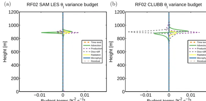
Figure 7.Profiles ofθ_l02budget terms for the DYCOMS-II RF02 drizzling stratocumulus case, time-averaged over the last hour (hour 6) of

the simulation, for(a)SAM LES and(b)CLUBB SCM. The profiles of overall time tendency are orange dashed-dotted lines, the advection

terms are green solid lines, and the production terms are purple dashed lines. The sum of the dissipation and diffusion terms are gray dashed lines. The microphysics (precipitation) terms are blue solid lines, the radiation terms are yellow solid lines, and the residuals are brown dashed-dotted lines. The microphysics term is negligible in both SAM LES and CLUBB. In this respect, both models match, as desired.

cloud fraction (RICO). Can CLUBB’s formulas approximate the microphysical (co)variance terms produced by SAM LES in other cloud cases? To begin to address this question, we simulate a boundary-layer case that has a layer-averaged rainwater mixing ratio that is comparable to that of RICO but that has a cloud fraction and precipitation fraction of nearly one. The case we simulate is the DYCOMS-II RF02 marine stratocumulus case.

In the SAM LES budgets of DYCOMS-II RF02 for r_t02

(Fig. 6a) andθ_l02(Fig. 7a), the microphysics term is negligi-ble in comparison to the other terms. While CLUBB’s dis-sipation and production terms are overestimated, CLUBB’s microphysics term is also negligible for both r_t02 (Fig. 6b) and θ_l02 (Fig. 7b), in agreement with SAM LES. In addi-tion, both SAM and CLUBB show similarly negligible mi-crophysics terms in the w0_r0

t, w0θl0, and r 0

tθl0 budgets (not

shown). This agreement suggests that CLUBB’s microphys-ical (co)variance formulas are applicable for shallow cloud cases with either small or large values of cloud fraction.

Why are the microphysics budget terms so much less sig-nificant in DYCOMS-II RF02 than they are in RICO? Con-sider the covariance of a field and a microphysics process rate – for example, the covariance ofθl and accretion rate. The magnitude of this covariance is related, in part, to the magnitude of θ_l02 and the magnitude of the variance of ac-cretion rate. (We set aside the issue of the correlation be-tween the two fields.) Comparing SAM LES results at al-titudes where precipitation is large, both θ_l02 and r_t02 are smaller in DYCOMS-II RF02 than in RICO (not shown). This is because marine stratocumulus cloud layers are well mixed by turbulence. DYCOMS-II RF02 also exhibits less variability in microphysical process rates. The variance of

warm-rain microphysics process rates is related, in part, to the variance of rainwater mixing ratio. In RICO, precipita-tion is found over a small region of the horizontal domain, while in the overcast DYCOMS-II RF02 case, precipitation is found over almost the entire horizontal domain. The in-precipitation mean ofrris much larger in RICO than it is in DYCOMS-II RF02 (not shown). Additionally, in RICO the ratio of thein-precipitationvariance to the square of the in-precipitationmean forrr(≈5) is much larger than the

corre-sponding ratio (_.1) in DYCOMS-II RF02. As a result, both the in-precipitation variance and the layer-mean variance of

rr is much greater in RICO than in DYCOMS-II RF02. In

summary, the microphysical (co)variance terms are smaller in marine stratocumuli than in cumuli partly because both the thermodynamic and microphysical fields are more homoge-neous in marine stratocumuli.

4.3 RICO sensitivity study: how significant are the microphysical (co)variance terms?

If the microphysical terms in the (co)variance equations are omitted, how large are the resulting errors? To address this, a second CLUBB simulation of RICO was run that is identi-cal to the original simulation with the one exception that the microphysical (co)variance terms are turned off.

(13)

−1 −0.5 0 0.5 1 x 10−9 0

500 1000 1500 2000 2500 3000 3500 4000

RICO CLUBB r variance budget t

Height [m]

(a)

−5 0 5

x 10−4

0 500 1000 1500 2000 2500 3000 3500 4000

RICO CLUBB θ_l variance budget

Height [m]

(b)

−1 −0.5 0 0.5 1

x 10−6

0 500 1000 1500 2000 2500 3000 3500 4000

RICO CLUBB r flux budget t

Height [m]

(c)

−1 −0.5 0 0.5 1

x 10−3

0 500 1000 1500 2000 2500 3000 3500 4000

RICO CLUBB θ

l flux budget

Height [m]

(d)

Figure 8.Profiles of budget terms for(a)r_t02,(b)θ_l02,(c)w0r_t0, and(d)w0θ_l0for the RICO precipitating shallow cumulus case, time-averaged over the last half (36 h) of the simulation (minutes 2160 through 4320), for CLUBB with the effects of microphysics on variances and covariances disabled. The profiles of overall time tendency are orange dashed-dotted lines, the advection terms are green solid lines, and the production terms are purple dashed lines. The sum of the buoyancy and pressure terms are the red solid lines. The diffusion (or the sum of diffusion and dissipation) terms are gray dashed lines, the microphysics (precipitation) terms are blue solid lines, and the residuals are brown dashed-dotted lines. Disabling the microphysical (co)variance terms greatly alters the budget balances for those fields. For the scalar

variances(a, b), both dissipation and advection increase in magnitude.

CLUBB simulation with microphysics feedback enabled in Figs. 3b and 4b, respectively, the terms from the simulation with microphysics feedback disabled are all much larger in magnitude. Within the cloudy layer, microphysics is a domi-nant sink of scalar variances. In order to compensate for the loss of that sink term, both dissipation and advection (be-low 3000 m) increase in (negative) magnitude. Since the in-tegral of the (turbulent) advection term over the vertical pro-file must have a mass-weighted vertical integral of 0, it be-comes an excessive source of r_t02andθ_l02above 3000 m. In essence, when the microphysical sink of variance is removed, the layer becomes more variable, develops more turbulence, and grows deeper. Similar characteristics are exhibited in the budget ofr_t0θ_l0(not shown).

The budgets of turbulent fluxes w0_r0

t andw0θl0 are shown

for the CLUBB simulation with microphysics terms dis-abled in Fig. 8c and d, respectively. When compared to

the same budgets from the CLUBB simulation with micro-physics terms enabled in Figs. 1b and 2b, respectively, the buoyancy+pressure terms, the advection terms, and thew0_r0 t

production term all increase in magnitude. This increase is relatively small, however, which is expected because micro-physics is a less significant term in the turbulent flux budgets. The terms from the simulation with microphysics terms dis-abled extend much higher in altitude, again because the layer has more vigorous turbulence.

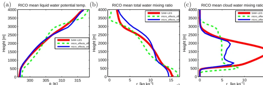
The errors induced by the loss of the microphysical (co)variance terms propagate throughout the model solu-tion, infecting, for instance, the mean fields. Figure 9 shows profiles of mean fields in a three-way comparison between (1) SAM LES, (2) CLUBB with microphysical effects on (co)variances disabled, and (3) CLUBB with microphysical effects on (co)variances enabled. In Fig. 9a, when the micro-physical effects on (co)variances are turned off, CLUBB’s

(14)

300 305 310 315 0

500 1000 1500 2000 2500 3000 3500 4000

RICO mean liquid water potential temp.

θ_l [K]

Height [m]

SAM−LES micro_effects_off micro_effects_on

(a)

0 5 10 15

x 10−3 0

500 1000 1500 2000 2500 3000 3500 4000

RICO mean total water mixing ratio

r [kg kg ]

t

Height [m]

(b)

0 5 10 15

x 10−6 0

500 1000 1500 2000 2500 3000 3500 4000

RICO mean cloud water mixing ratio

r [kg kg ]

c

Height [m]

(c)

–1 –1

Figure 9.Profiles of(a)θl,(b)rt, and(c)rcfor the RICO precipitating shallow cumulus case, time-averaged over the last half (36 h) of the simulation (minutes 2160 through 4320). The red solid lines are SAM LES results, the blue solid lines are CLUBB with the effects of

microphysics on the variances and covariances (w0r_t0,w0θ_l0,r_t02,θ_l02, andr_t0θ_l0) enabled, and the green dashed lines are CLUBB with the effects

of microphysics on the aforementioned variances and covariances turned off. Disabling the microphysical feedbacks into the (co)variances

produces aθlprofile that is too warm at lower altitudes and too cool aloft when compared to SAM LES. This is because turning off the

microphysical damping increases the vigor of the layer. As a result, cloud water is found at altitudes higher than it is found in SAM LES.

As a result of the cooler temperatures and excessive turbu-lence aloft, Fig. 9c shows thatrcextends too high in altitude when compared to SAM LES. Omitting the microphysical (co)variance terms would constitute a significant model er-ror.

5 Conclusions

Microphysical sources and sinks of (co)variances involving total water and liquid water potential temperature are signif-icant. A LES of the RICO shallow cumulus case shows that, in this cloud case, microphysical sources and sinks are ma-jor terms in the budgets of variances and turbulent fluxes. In particular, microphysical processes have three main effects. First, precipitation formation and growth is the major sink of r_t02, θ_l02, and the magnitude of r_t0θ_l0 in the upper half of the cloud layer (see Figs. 3, 4, and 5). In particular, micro-physical damping is greater than turbulent dissipation. The damping of scalar variances occurs because rain formation depletes cloud water preferentially in the moistest part of the cloud. This depletion preferentially reduces the largest val-ues of (liquid) cloud water, thereby reducing the horizontally averaged variance. Second, microphysics also damps the tur-bulent flux of scalars,w0_r0

tandw0θl0(see Figs. 1 and 2). The

mechanism is the same: precipitation reduces cloud water in the moistest part of the cloud, which also contains stronger updrafts. Although the effects of microphysics on fluxes are smaller than those on variances, microphysics is still a ma-jor term in the w0_θ0

l budget and ought not to be ignored.

Third, evaporation of rain below cloud acts as a source ofθ_l02. The positive sign arises because evaporation of rain cools the cooler part of the subcloud layer. This evaporation-induced generation ofθ_l02 is a key aspect of cold pool formation. It

leads to buoyant generation ofw0_θ0

l below cloud base, which

in turn leads to new convection.

This paper demonstrates that all these microphysical sources and sinks can be calculated analytically, given a suf-ficiently simple warm-rain microphysics scheme and a suffi-ciently simple multivariate PDF. These analytic expressions have been implemented in the predictive equations for vari-ances and covarivari-ances involving rt and θl in the CLUBB

parameterization. When applied in an interactive, single-column simulation of the RICO case by CLUBB, the micro-physical terms agree qualitatively with LES in sign and in relative magnitude.

In the future, analytic integration of microphysical sources of scalar (co)variances may provide a useful step for the parameterization of cold pools and cloud organization. It does not parameterize cold pools and cloud organization di-rectly, because it does not account for spatial arrangement of cloud parcels. Furthermore, it does not even parameter-ize all effects of cold pools and cloud organization. How-ever, it does parameterize effects that are directly related to scalar variability, and it parameterizes these effects in a non-phenomenological, rigorous way. Namely, it defines the mi-crophysical sources with precise, mathematical expressions, and it provides explicit formulas for the case of idealized, warm-rain microphysics. Although the effects of cold pools are relatively modest in the statistically steady, shallow-cumulus case analyzed in this paper, the effects are larger in some transient, deep convective cases (e.g., Khairoutdinov and Randall, 2002, 2006).

(15)

sampling noise or other integration errors. More importantly, analytic integration provides an alternative solution that can be used to test whether a Monte Carlo integration code con-verges to the correct solution (Larson and Schanen, 2013). In past experience, we have found such testing to be crucial. Bugs are surprisingly easy to introduce, and without com-parison against an independent solution, results produced by a Monte Carlo integrator will be subject to lingering doubts. On the other hand, once a Monte Carlo integrator has been tested against an analytic solution, it can be used more con-fidently with a comprehensive microphysics scheme that in-cludes ice in order to simulate a variety of shallow and deep cloud cases. In fact, this has already been done in Storer et al. (2015). In this way, analytic integration of the microphysical effects on scalar variances and fluxes is an enabling technol-ogy: it enables the verification of general subgrid integration methods.

6 Code availability

(16)

Appendix A: Covariances involving microphysics process rates

This Appendix sets up the integrals that need to be solved in order to find the microphysical covariance terms listed in Sect. 2.1. The integrals set up here can be evaluated using the expressions given in the Supplement.

The nine microphysical covariances involving each ofw,

rt, andθlwith each of KK autoconversion rate, accretion rate,

and evaporation rate are calculated by integrating over the PDF. The KK microphysics process rates are calculated, in part, based on variables that involve saturation, such as rc. In order to calculate quantities that involve saturation, a PDF transformation, which is a change of coordinates, is required. The multivariate PDF undergoes stretching, translation, and rotation of the axes (Larson et al., 2005; Mellor, 1977). An independent PDF transformation takes place in each PDF component. Ultimately,rt andθlare replaced in the PDF by

χ andη, whereχis an “extended” liquid water mixing ratio that has a positive value when air is supersaturated. In this scenario,χ is also equal torc. When air is subsaturated, χ

has a negative value. The variableηis orthogonal toχ. Please note that several prior publications denote these variables as

s andt (e.g., Larson et al., 2005, 2002; Mellor, 1977). The transformations that relatertandθltoχandηare

crt(i) rt−µrt(i)

₌ η−µη(i)

+ χ−µχ (i)

2 ,and (A1)

cθl(i) θl−µθl(i)

= η−µη(i)

− χ−µχ (i)

2 , (A2)

whereµrt(i)is the mean ofrtin theith PDF component and

µθl(i)is the mean ofθlin theith PDF component.

The mean ofχin theith PDF component,µχ (i), is given

by

µχ (i)=

µrt(i)−rsw µTl(i), p

1+3 µTl(i)

rsw µTl(i), p

, (A3)

wherersw µTl(i), p

is the saturation mixing ratio with re-spect to liquid water,µTl(i)is the mean ofTl in theith PDF component (calculated fromµθl(i)), and3 µTl(i)

is given by

3 µTl(i)

=Rd

Rv

_L

v RdµTl(i)

Lv CpdµTl(i)

, (A4)

whereRvis the gas constant for water vapor. The mean ofη

in theith PDF component,µη(i), ultimately does not factor

into the solution to the integral equations. Its value is irrele-vant and can be set to an arbitrary value, such as 0, for sim-plicity. However, it should be noted that the PDF component standard deviations ofηand PDF component correlations in-volvingηstill factor into the solution. The coefficientscrt(i) andcθl(i)are given by

crt(i)=

1 1+3 µTl(i)

rsw µTl(i), p

,and (A5)

cθl(i)=

1+3 µT_l(i)

µrt(i)

3 µT_l(i)

rsw µT_l(i), p

1+3 µTl(i)

rsw µTl(i), p

2

C_pd

Lv

p p0

R_d C_pd

.

(A6) Theith PDF component variance ofχ is found by squar-ing the difference of Eq. (A1) and Eq. (A2), and then aver-aging the result. Likewise, theith PDF component variance ofηis found by squaring the sum of Eq. (A1) and Eq. (A2), and then averaging the result. Theith PDF component corre-lation ofχ andηcan be found using a similar method. See Larson et al. (2005) for more details.

A1 Covariances involving autoconversion rate

The general form of the KK equation for autoconversion rate is the product of a coefficient (Cauto) andr_cαNcβ (where for

KK,α=2.47 andβ= −1.79). The integral equation for the covariance ofw and autoconversion rate involves the PDF variablesw,rt,θl, andNcn. The equation is

w0∂rr ∂t

0

auto

=

∞ Z

−∞ ∞ Z

0

w−w

_∂rr

∂t _auto

− ∂rr

∂t _auto

!

×P (w, rt, θl, Ncn)dNcndθldrtdw. (A7) The PDF is transformed (in each component) from rt and

θl coordinates to χ and η coordinates. Additionally, rc=

χ H (χ )andNc=NcnH (χ ), whereH (χ )is the Heaviside step function (Griffin and Larson, 2016). The equation be-comes

w0∂rr ∂t

0

auto

=

n X

i=1 ξ(i)

∞ Z

−∞ ∞ Z

0

w−w

× CautoχαNcnβ(H (χ ))α+β − ∂rr

∂t _auto

!

×P(i)(w, χ , η, Ncn)dNcndηdχdw, (A8)

where the coefficientCauto=1350 10−6ρdβ, and whereρd

is the density of dry air. For CLUBB’s PDF,n=2. The vari-ableηcan be integrated out of the PDF. The equation for the covariance ofwand autoconversion rate is

w0∂rr ∂t

0

auto

=

Cauto n X

i=1 ξ(i)

∞ Z

−∞ ∞ Z

0

w−w

(17)

× χαNcnβ(H (χ ))α+β − 1 Cauto ∂rr ∂t auto !

×PNNL(i)(w, χ , Ncn)dNcndχdw, (A9)

where PNNL(i)(w, χ , Ncn) is the ith component trivariate

PDF involving two normal variates and one lognormal vari-ate. The functional form of the PDF (for theith PDF compo-nent) is given in the Supplement in Eq. (S2), and the integral is solved (for theith PDF component) in Sect. S6 (Eqs. S25 through S32).

The integral equation for the covariance ofrtand autocon-version rate involves the PDF variablesrt,θl, andNcn. The equation is

r_t0∂rr ∂t 0 auto = ∞ Z −∞ ∞ Z −∞ ∞ Z 0

rt−rt ∂rr ∂t _auto − ∂rr ∂t _auto !

×P (rt, θl, Ncn)dNcndθldrt. (A10) During the PDF transformation, Eq. (A1) is used to substitute forrt. The equation becomes

r_t0∂rr ∂t 0 auto = n X

i=1 ξ(i) ∞ Z −∞ ∞ Z −∞ ∞ Z 0

µrt(i)−rt+

η−µη(i)

+ χ−µχ (i)

2crt(i)

× CautoχαNcnβ(H (χ ))α+β − ∂rr ∂t _auto !

×P(i)(η, χ , Ncn)dNcndχdη. (A11)

The integral equation is split and simplified, and becomes

r_t0∂rr ∂t 0 auto = Cauto n X i=1 ξ(i) ×   1 2crt(i)

∞ Z −∞ ∞ Z −∞ ∞ Z 0

η−µη(i)

× χαNcnβ(H (χ ))α+β −

1 Cauto ∂rr ∂t _auto !

×PNNL(i)(η, χ , Ncn)dNcndχdη

+ 1

2crt(i)

∞ Z 0 ∞ Z 0

χα+1NcnβPNL(i)(χ , Ncn)dNcndχ

+

µrt(i)−rt−

µχ (i)

2crt(i)

× ∞ Z 0 ∞ Z 0

χαNcnPNLβ (i)(χ , Ncn)dNcndχ 

, (A12)

wherePNL(i)(χ , Ncn)is theith component bivariate PDF

in-volving one normal variate and one lognormal variate. The functional form of the trivariate NNL PDF (for theith PDF component) is given in the Supplement in Eq. (S2), and the related integral is solved (for the ith PDF component) in Sect. S6 (Eqs. S25 through S32). The functional form of the bivariate NL PDF (for theith PDF component) is given in Eq. (S5), and the related integrals are solved (for theith PDF component) by using the general form given in Sect. S8 (Eqs. S41 through S44).

The integral equation for the covariance ofθland

autocon-version rate involves the PDF variablesrt,θl, andNcn. The equation is

θ_l0∂rr ∂t 0 auto = ∞ Z −∞ ∞ Z −∞ ∞ Z 0

θl−θl

_∂r r ∂t auto

− ∂rr

∂t auto !

×P (rt, θl, Ncn)dNcndθldrt. (A13)

During the PDF transformation, Eq. (A2) is used to substitute forθl. The equation becomes

θ_l0∂rr ∂t 0 auto = n X i=1 ξ(i) ∞ Z −∞ ∞ Z −∞ ∞ Z 0

µθl(i)−θl+

η−µη(i)

− χ−µχ (i)

2cθl(i)

× CautoχαNcn(H (χ ))β α+β − ∂rr

∂t auto !

×P(i)(η, χ , Ncn)dNcndχdη. (A14)

The integral equation is split and simplified, and becomes

θ_l0∂rr ∂t 0 auto = Cauto n X i=1 ξ(i) ×   1 2cθl(i)

∞ Z −∞ ∞ Z −∞ ∞ Z 0

η−µη(i)

× χαNcnβ(H (χ ))α+β −

1 Cauto ∂rr ∂t _auto !

×PNNL(i)(η, χ , Ncn)dNcndχdη

− 1

2cθl(i)

∞ Z 0 ∞ Z 0

χα+1NcnβPNL(i)(χ , Ncn)dNcndχ

+

µθl(i)−θl+

µχ (i)

2cθl(i)

× ∞ Z 0 ∞ Z 0

χαNcnPNLβ (i)(χ , Ncn)dNcndχ 