www.geosci-model-dev.net/4/1011/2011/ doi:10.5194/gmd-4-1011-2011
© Author(s) 2011. CC Attribution 3.0 License.
Geoscientific
Model Development
Development of an ensemble-adjoint optimization approach to
derive uncertainties in net carbon fluxes
T. Ziehn1, M. Scholze1, and W. Knorr1,2
1Department of Earth Sciences, University of Bristol, Wills Memorial Building, Queen’s Road, Bristol, BS8 1RJ, UK 2Department of Meteorology and Climatology, Aristotle University of Thessaloniki, 54124 Thessaloniki, Greece
Received: 9 June 2011 – Published in Geosci. Model Dev. Discuss.: 8 July 2011
Revised: 3 November 2011 – Accepted: 9 November 2011 – Published: 18 November 2011
Abstract. Accurate modelling of the carbon cycle strongly depends on the parametrization of its underlying processes. The Carbon Cycle Data Assimilation System (CCDAS) can be used as an estimator algorithm to derive posterior parame-ter values and uncertainties for the Biosphere Energy Trans-fer and Hydrology scheme (BETHY). However, the simulta-neous optimization of all process parameters can be challeng-ing, due to the complexity and non-linearity of the BETHY model. Therefore, we propose a new concept that uses en-semble runs and the adjoint optimization approach of CC-DAS to derive the full probability density function (PDF) for posterior soil carbon parameters and the net carbon flux at the global scale. This method allows us to optimize only those parameters that can be constrained best by atmospheric car-bon dioxide (CO2) data. The prior uncertainties of the
re-maining parameters are included in a consistent way through ensemble runs, but are not constrained by data. The final PDF for the optimized parameters and the net carbon flux are then derived by superimposing the individual PDFs for each ensemble member. We find that the optimization with CCDAS converges much faster, due to the smaller number of processes involved. Faster convergence also gives us much increased confidence that we find the global minimum in the reduced parameter space.
1 Introduction
The terrestrial biosphere plays an important role in the global carbon cycle and has a great impact on the accumulation of carbon dioxide (CO2) in the atmosphere. Feedbacks between
the carbon cycle and climate change, generally known as carbon-climate feedbacks, have the potential to accelerate the
Correspondence to: T. Ziehn ([email protected])
rise in atmospheric CO2, which causes further global
warm-ing (Matthews et al., 2007). The quantification of the carbon cycle-climate feedback is therefore important for determin-ing the magnitude of future climate change. However, there is much uncertainty about the size of natural sinks of the ter-restrial carbon cycle, which in turn has a major impact on the uncertainty of climate predictions (Zaehle et al., 2005; Denman et al., 2007). The large variations in the prediction of the future atmospheric CO2load result from differences
between models (Cramer et al., 1999; Friedlingstein et al., 2006), but also from uncertainties of the process parame-ters of the terrestrial ecosystem models (TEMs) (Knorr and Heimann, 2001).
The increase in the complexity of TEMs over recent years has also led to an increase in the number of parameters. Prior parameter values are usually based on “expert knowl-edge”, which in some cases is little more than an informed guess. Furthermore, even those parameters that have clear analogues iin the observed system are often not directly re-lated to the values derived from laboratory experiments or site-scale experiments. Parameter optimization methods are very useful in this context: they provide a way of constrain-ing the model parameters against observations and in this way reduce parameter uncertainties.
size which is not always feasible due to computational lim-itations (i.e. long computing time of TEMs). Variational data assimilation, such as the four-dimensional variational scheme (4-D-Var), allows one to combine observational data with a model. It uses derivative code (i.e. the adjoint of the model) for the optimization of the parameters and therefore requires the model to be differentiable with respect to all pa-rameters. Although the 4-D-Var approach is very efficient in most cases, the optimization might not always converge in time or might only identify a local minimum. These is-sues arise due to the complexity and non-linearity of state-of-the-art TEMs and the potentially high-dimensional parame-ter space.
In this contribution we address the convergence is-sue of the optimization scheme in the 4-D-Var approach as used in the Carbon Cycle Data Assimilation System (CCDAS) (Rayner et al., 2005) and propose a new con-cept for deriving the posterior PDF for parameters and target quantities in a global TEM. Although we focus only on one TEM, the Biosphere Energy Transfer and Hydrology scheme (BETHY) (Knorr, 2000), the approach is universal and can be applied to any other model. The main idea is that we only optimize a subset of parameters, i.e. those controlling the heterotrophic respiration (in the following called soil car-bon parameters), because they are best constrained by atmo-spheric CO2concentration observations as demonstrated by
Rayner et al. (2005) and Scholze et al. (2007). The prior uncertainties of the remaining parameters, i.e. those related to net primary productivity (NPP), are included through en-semble runs and are therefore not constrained by the obser-vations. This new concept allows us to treat all parameter uncertainties in a consistent way.
2 Materials and methods
The 4-D-Var data assimilation scheme has been successfully applied within CCDAS to constrain process parameters in a TEM. CCDAS can be used in various modes. For exam-ple, in calibration mode it serves as an estimator algorithm for a set of photosynthesis, autotrophic and heterotrophic respiration process parameters by using automatically gen-erated adjoint code (first derivative) for parameter optimiza-tion. In Hessian mode, the Hessian model code (second order derivative) is used for estimating posterior parameter uncer-tainties. As its ecosystem model, CCDAS uses the BETHY model, which simulates carbon assimilation and soil respi-ration within a full energy and water balance and phenology scheme. Calculated fluxes are then mapped to atmospheric concentrations using the atmospheric transport model TM2 (Heimann, 1995).
The CCDAS framework has been previously described in detail by Scholze (2003) and Rayner et al. (2005). Therefore, we provide only a brief summary. The data assimilation in CCDAS is performed in two steps: In the first step, the full BETHY model is used to assimilate global monthly fields of
the fraction of Absorbed Photosynthetically Active Radiation (fAPAR) for optimizing parameters controlling soil moisture and phenology (Knorr and Schulz, 2001). In the second step, soil moisture and leaf area index (LAI) fields are provided as inputs for a reduced version of BETHY, in the follow-ing referred to as CarbonBETHY. This version is used to as-similate atmospheric CO2 concentration observations from
a large number of observation stations for optimizing pho-tosynthesis and soil carbon parameters and to derive their posterior uncertainties (Rayner et al., 2005; Scholze et al., 2007).
2.1 Data assimilation
The Bayesian approach (Tarantola, 1987, 2005) provides a consistent framework for constraining model parametersx
against observationsc. This framework enables us to com-bine the prior probability distribution of the parametersP (x) with the probability distribution of the observations given the parametersP (c|x)in order to determine the inverse (poste-rior) probability distribution of the parameters given the ob-servationsP (x|c):
P (x|c)= 1
AP (c|x)P (x). (1)
The factor 1/A is a normalisation constant and in-dependent of the parameters x. In many cases a normal distribution is assumed for the prior parameter values and the observations. This Gaussian assumption has the advantage that only the mean and covariance have to be provided in order to describe the prior probability distribution of each variable. Applying a normal distribution to Eq. (1) leads to the following expression:
P (x|c)= 1 Aexp
−1
2(cM−c)
TC−1
c (cM−c)
exp
−1
2(x−x0)
TCx 0
−1(x−x 0)
, (2)
wherecM=M(x)are the modelled observations. The
co-variance matrices Ccand Cx0 express the uncertainty of the observations cand the model parameter priors x0,
respec-tively. We are usually interested in the maximum ofP (x|c), which will give us the most likely set of parameter values. This can be found in two ways: we can either maximize Eq. (2) using Monte Carlo inversion, or we can minimize the negative exponent of Eq. (2) using variational data assimila-tion.
The cost functionJ (x) P (x|c)= 1
Aexp(−J (x)) (3)
J (x)=1 2
(cM−c)TCc−1(cM−c)
+(x−x0)TCx0
−1(x−x 0)
(4)
describes the mismatch between the observations and their modelled equivalents and the mismatch between the param-eters and their priors.
The data assimilation in CCDAS is based on the 4-D-Var scheme. In our case, the vector of observations, c, repre-sents monthly atmospheric CO2concentrations measured at
41 remote monitoring stations (GLOBALVIEW-CO2, 2004).
CarbonBETHY is used to calculate surface fluxes which are then mapped via the atmospheric transport model TM2 to atmospheric concentrations cM. Since BETHY calculates
only the natural land-atmosphere fluxes, we have to add land use change as an external flux as described in Rayner et al. (2005). Background fluxes for fossil fuel emissions are based on the flux magnitudes from Boden et al. (2009) as described in Scholze et al. (2007). The spatial flux pattern and the magnitude of ocean CO2exchange is taken from Takahashi
et al. (1999) with estimates of inter annual variability taken from Le Qu´er´e et al. (2007).
The parameter vector x contains the photosynthesis and soil carbon parameters in CarbonBETHY with their prior values represented by x0 (see Tables S1 and S2).
A quasi-Newton method, the Broyden-Fletcher-Goldfarb-Shanno (BFGS) variant of the Davidon-Fletcher-Powell (DFP) formula (Fletcher and Powell, 1963; Press et al., 1996), is used for the minimization of the cost function, which requires the calculation of the gradient ofJ with re-spect to the control parametersxin each iteration. All deriva-tive code is generated from the model’s source code using the tool Transformation of Algorithms in Fortran (TAF) (Giering and Kaminski, 1998; Kaminski et al., 2003).
2.2 Challenges
The simultaneous optimization of the photosynthesis and soil carbon parameters in CCDAS as described in the previous section can be challenging due to slow convergence or fail-ure of convergence. Even if a convergence requirement is fulfilled (i.e. test for convergence on1x), the gradient of the cost function may not be sufficiently close to zero at the final convergence point in parameter space. As a consequence the Hessian is not positive definite (i.e. contains negative eigen-values), which indicates that an exact minimum has not been found. This has been noted by Rayner et al. (2005) where, in order to derive the posterior parameter uncertainties, the Hessian had to be modified manually. Another concern is that due to the large input space dimension and the fact that the BETHY model is highly non-linear, it is likely that we only identify a local minimum with CCDAS.
The study by Ziehn et al. (2011a) has revealed that the per-formance of the optimization in CCDAS can be significantly improved if only the soil carbon parameters are constrained with atmospheric CO2concentration data, while all
param-eters controlling NPP were kept fixed. Earlier studies with CCDAS (Rayner et al., 2005; Scholze et al., 2007) confirmed that NPP-related parameters (i.e. photosynthesis parameters)
are constrained relatively little by the assimilation of CO2
concentration observations. Most importantly it could be shown in the study by Ziehn et al. (2011a) that an ensem-ble run of optimizations, starting each of them in a different point, identified only one minimum in the physical parameter space, which gives us additional confidence that the global minimum has been found. Additionally, the gradient in the cost function minimum was very close to zero and the Hes-sian was positive definite so that no manual modification of the Hessian was required. Although the overall performance of the optimization has improved significantly, there is one drawback of the technique presented in their work: the un-certainties in the NPP-related parameters have not been in-cluded, which means that estimated uncertainties of the soil carbon parameters and diagnostics were only a lower bound. Therefore, we propose a new concept, that treats the uncer-tainties in the photosynthesis parameters via ensemble runs and optimizes the soil carbon parameters using the adjoint optimization approach within CCDAS.
2.3 Concept and test case
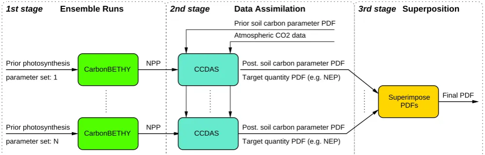
A flow chart of the concept developed in this contribution is presented in Fig. 1. In a first stage, ensemble runs are per-formed using CarbonBETHY by varying the NPP-related pa-rameters randomly according to a normal distribution defined by their prior mean and standard deviation (see Table S1). All other parameters (i.e. soil carbon parameters) are kept fixed. Here, we use a sample size ofN=200. We also per-form one additional forward run, referred to as base case, where all NPP controlling parameters are set to their prior mean.
CarbonBETHY is driven by observed climate data over 25 yr for the period 1979 to 2003. Global vegetation is mapped onto 13 different plant functional types (PFTs) and each grid cell can contain sub-areas (sub-grid cells) with up to three different PFTs with their amount specified by each PFT’s fractional cover. CarbonBETHY is run on a 2◦×2◦ grid with 3462 land grid cells (excl. Antarctica).
Each ensemble run (including the base case) provides a monthly field of NPP, which is used as an input field in the second stage. Here, we apply CCDAS to optimize only the soil carbon parameters, using atmospheric CO2
parameter set: 1
parameter set: N
Prior photosynthesis NPP
NPP
CCDAS
CCDAS
Target quantity PDF (e.g. NEP) Post. soil carbon parameter PDF Target quantity PDF (e.g. NEP) Post. soil carbon parameter PDF
Superimpose PDFs
Final PDF
Prior photosynthesis
Atmospheric CO2 data Prior soil carbon parameter PDF
CarbonBETHY
CarbonBETHY
1st stage Ensemble Runs 2nd stage Data Assimilation 3rd stage Superposition
Fig. 1.
Flow chart of the ensemble-adjoint optimization approach.
13
Fig. 1. Flow chart of the ensemble-adjoint optimization approach.model within CCDAS (Scholze et al., 2007). Thus we ob-tain uncerob-tainty estimates and covariances for output target quantities, such as the net ecosystem productivity (NEP) cal-culated as
NEP=NPP−RS=NPP−(RS,s+RS,f), (5)
whereRS,sandRS,fare the respiration fluxes from the slowly
and rapidly decomposing soil carbon pools, respectively. In a third stage, we superimpose the posterior PDFs for the soil carbon parameters and the output target quantity in order to obtain their final PDF, which also accounts for the prior uncertainties in the NPP-related parameters. The calculation of the final PDFp(y)for the output target quantityyis given by the following equations:
p(y)=p 0(y)
N (6)
p0(y)=
N
X
i=1
1
q
2π σi2
exp −(yi−µi)
2
2σi2
!
, (7)
whereN is the ensemble size andµi andσi are the mean
and standard deviation for each individual outputyi.
Indi-vidual PDFs described byµi andσi have a normal
distri-bution. In practice, we discretize those PDFs using a step length of 1×10⁻⁴PgC and then calculate the sum over all discrete points divided by the total numberN of PDFs (en-semble size). In this way we obtain the final PDF as de-scribed by Eqs. (6) and (7), which can be non-Gaussian. The calculation of the final (superimposed) soil carbon parameter PDF is performed in a similar way.
3 Results and discussion
The optimization within CCDAS (data assimilation in stage 2, see Fig. 1) reached convergence for 198 out of the
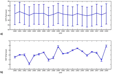
200 ensemble members and required about 1700 iterations on average. However, of the 198 successful optimization runs we had to exclude further 28 runs, where either the gra-dient in the cost function minimum was not sufficiently small enough (i.e. greater than 1×10⁻³) or the optimal (posterior) parameter set contained non-physical parameter values. For physically meaningful results we require here that all param-eters are positive, and some paramparam-eters that respresent frac-tions have to fall between 0 and 1. However, the optimal set of parameters derived by CCDAS may contain values out-side those defined ranges and we therefore have to exclude the corresponding runs. This leaves us with 170 sets of op-timal soil carbon parameters, which were obtained by using 170 different NPP input fields (ensemble runs in stage 1, see Fig. 1). A time series of global mean NPP including error bars is shown in Fig. 2a.
A list of the posterior parameter values for the five global parameters including their uncertainties is presented in Ta-ble 1, the values for the parameterβ for each PFT and re-gion and the offset (global atmospheric CO2 concentration
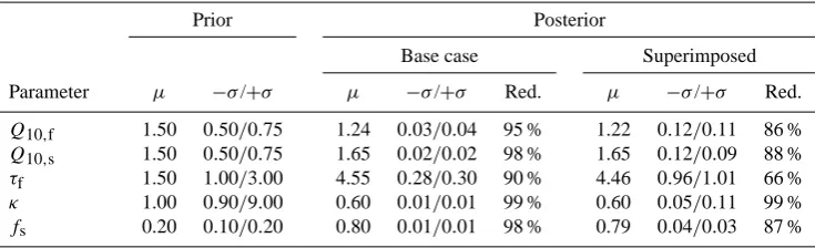
at the beginning of the optimization period) are presented in Table S2. Note that we distinguish between model pa-rameters (physical domain) and papa-rameters as used by the optimization in CCDAS (normalized domain). For most of the parameters we assume a log-normal distribution to en-sure positive values as discussed above, which results in the asymmetry shown in Table 1 and Table S2. However, af-ter suitable transformation, all parameaf-ters follow a Gaussian distribution in the normalized domain. Results are only dis-cussed in the physical domain and in the following, we focus only on the five global parameters. The optimal values for the temperature sensitivity of respiration for the fast and slow carbon pools (Q10,fandQ10,s) for the base case are close to
their prior values and within the prior uncertainty range. The soil moisture dependence parameterκis reduced from its ini-tial value, but is also within its prior uncertainty range. The
1980 1981 1982 1983 1984 1985 1986 1987 1988 1989 1990 1991 1992 1993 1994 1995 1996 1997 1998 1999 50
55 60 65 70 75 80
NPP [PgC/year]
year
1980 1981 1982 1983 1984 1985 1986 1987 1988 1989 1990 1991 1992 1993 1994 1995 1996 1997 1998 1999 −1
0 1 2 3 4 5
NEP [PgC/year]
year
a)
b)
Fig. 2.Time series of (a) the global mean net primary productivity (NPP) and (b) the global mean net ecosystem
productivity (NEP). For (a) the median and error bars are calculated from the 170 NPP fields for each year,
which are then used as inputs for CCDAS. For (b) the median and error bars are based on the final NEP PDF for
each year. Error bars represent the lower and upper percentiles equivalent to one standard deviation (i.e. 15.9th
percentile and 84.1th percentile respectively).
14
Fig. 2. Time series of (a) the global mean net primary productivity (NPP) and (b) the global mean net ecosystem productivity (NEP). For (a) the median and error bars are calculated from the 170 NPP fields for each year, which are then used as inputs for CCDAS. For (b) the median and error bars are based on the final NEP PDF for each year. Error bars represent the lower and upper percentiles equivalent to one standard deviation (i.e. 15.9th percentile and 84.1th percentile, respectively).
1.7 1.75 1.8 1.85 1.9 1.95 2
0 10 20 30 40 50
Mean : 1.8296 Sigma : 0.013416 Skewness : 1.1886 Kurtosis : 7.2952
Mean : 1.8303 Sigma : 0.0093712
1980s
NEP [PgC/yr]
p [yr/PgC]
2.450 2.5 2.55 2.6 2.65
10 20 30 40 50 60 70 80
Mean : 2.5559 Sigma : 0.011646 Skewness : −0.20574 Kurtosis : 0.52795
Mean : 2.556 Sigma : 0.0054002
1990s
NEP [PgC/yr]
p [yr/PgC]
a)
b)
Fig. 3. PDFs for global NEP for(a)the 1980s and(b)the 1990s. Blue: 170 individual PDFs, red: base case
PDF (which used prior photosynthesis parameters and was not part of the ensemle), green: superimposed PDF
from the 170 individual PDFs.
Fig. 3. PDFs for global NEP for (a) the 1980s and (b) the 1990s. Blue: 170 individual PDFs, red: base case PDF (which used prior photosynthesis parameters and was not part of the ensemle), green: superimposed PDF from the 170 individual PDFs.
−1 −0.8 −0.6 −0.4 −0.2 0 0.2 0.4 0.6 0.8 1
1980 1981 1982 1983 1984 1985 1986 1987 1988 1989 1980
1981 1982 1983 1984 1985 1986 1987 1988 1989
a) b) 1990 1991 1992 1993 1994 1995 1996 1997 1998 1999
1990 1991 1992 1993 1994 1995 1996 1997 1998 1999
Fig. 4.Uncertainty correlation matrix of global mean NEP for(a)the 1980s and(b)the 1990s.
16
Fig. 4. Uncertainty correlation matrix of global mean NEP for (a) the 1980s and (b) the 1990s.
Table 1. Prior and posterior parameter values including their uncertainties for five global parameters. Upper and lower percentiles equivalent to one standard deviation are given (i.e.µ−σ is equivalent to the 15.9th percentile andµ+σ is equivalent to the 84.1th percentile). The relative reduction in uncertainty (Red.) related to+σis also shown. Prior and posterior parameter values for theβparameters are provided in Table S2. Units:τf, years; all others unitless.
Prior Posterior
Base case Superimposed
Parameter µ −σ/+σ µ −σ/+σ Red. µ −σ/+σ Red.
Q10,f 1.50 0.50/0.75 1.24 0.03/0.04 95 % 1.22 0.12/0.11 86 %
Q10,s 1.50 0.50/0.75 1.65 0.02/0.02 98 % 1.65 0.12/0.09 88 %
τf 1.50 1.00/3.00 4.55 0.28/0.30 90 % 4.46 0.96/1.01 66 %
κ 1.00 0.90/9.00 0.60 0.01/0.01 99 % 0.60 0.05/0.11 99 % fs 0.20 0.10/0.20 0.80 0.01/0.01 98 % 0.79 0.04/0.03 87 %
optimized parameter values for the fast pool turnover time, τf, and the fractionfsof the decomposition flux going from
the fast to the long-lived soil carbon pool are much larger than their priors and both outside the prior uncertainty range. All five global parameters are well constrained by the CO2
data, shown by the small posterior uncertainty in the base case. The posterior mean values for all soil carbon param-eters are very similar in both cases (base case and superim-posed case), showing that the mean values are not heavily effected by changes in the NPP-related parameters.
Our target output quantity is global mean NEP, for which a time series is shown in Fig. 2b. In the following we focus on global mean NEP for the 1980s and 1990s. The PDFs for those quantities are presented in Fig. 3. We obtain the final PDF by superimposing the 170 individual PDFs (Eq. 7) from each optimization run to account for both, the posterior soil carbon parameter uncertainties and the prior uncertain-ties in the NPP-related parameters. The superimposed PDF is not necessarily Gaussian. However, skewness and kurtosis of the distribution for the case of the 1990s (Fig. 3b) indi-cate that the assumption of a normal distribution is a good
approximation. The mean values for our target quantities are nearly identical for the base case and the superimposed case, showing again that the NPP-related parameters have little effect on the mean values. The uncertainties for the target quantities, however, increase by more than 50 % for the 1980s and by more than 100 % for the 1990s using the ensemble-adjoint method.
According to Denman et al. (2007) the terrestrial carbon sink removed −1.7 Pg C yr−1 (range: −3.4 to +0.2 Pg C yr−1) during the 1980s and −2.6 Pg C yr−1 (range: −4.3 to−0.9 Pg C yr−1) during the 1990s from the atmosphere. The results from our study match the mean values well, with a carbon flux of−1.83 Pg C yr−1 (range: −1.84 to−1.82 Pg C yr−1) for the decade of the 1980s and −2.55 Pg C yr−1 (range: −2.57 to−2.54 Pg C yr−1) for the decade of the 1990s. However, the uncertainties of our re-sults are small in comparison to those from Denman et al. (2007). One reason for this is the large number of negative entries for individual years in the error covariance matrix of global mean NEP for the 1980s and 1990s.
The covariance between the flux uncertainties can be ex-pressed via the uncertainty correlation matrix of diagnostics, Rd, which is defined as follows:
Rdi,j=
Cdi,j
σiσj
, (8)
whereCdi,j is elementi,j of the uncertainty covariance ma-trix of the diagnostics (global NEP per year), andσi the
pos-terior uncertainty of parameteri derived from the diagonal elements Cdi,i of the matrix Cd. Figure 4 shows the
cor-relation matrix for global mean NEP for the 1980s and the 1990s. Due to the large number of negative correlations the overall uncertainty for global mean NEP over the 10 yr pe-riod (1980s and 1990s) is rather small. However, the uncer-tainty for global mean NEP for a single year, for example the year 1990, is by at least a factor of two larger then global mean NEP for the 1990s in the base case and increases by the ensemble-adjoint method by more than a factor of four.
4 Conclusions
The ensemble-adjoint optimization approach presented here allows us to treat all parameter uncertainties in a TEM in a consistent way. Some parameters are constrained against data using the 4-D-Var data assimilation scheme, whereas the uncertainties of the remaining parameters are included via ensemble runs. In this way we optimize only those pa-rameters which are constrained best by the observations used in the 4-D-Var step, but retain full error propagation from parameters to diagnostics. This has the advantage that fewer parameters and processes are involved within the optimiza-tion process, which, in turn, speeds up the convergence of the optimization. We are also more confident that we find the global minimum in the reduced parameter space.
In this study we have illustrated the usefulness of the ensemble-adjoint optimization approach by including prior uncertainties of model parameters (here the NPP-related pa-rameters) that have not been constrained by the atmospheric CO2 data, to derive a full probability density function on
the model’s target output quantities. For future applications, the proposed concept also allows the inclusion of posterior uncertainties for the remaining, yet unconstrained parame-ters. Ziehn et al. (2011b) have demonstrated how to constrain the parameters of the Farquhar et al. (1980) photosynthesis model using an extensive set of plant traits and therefore pro-vide a way on how to derive the posterior PDF for the NPP-related parameters. Those results could potentially been used within the same ensemble-adjoint optimization framework. We would only need to replace the prior mean and uncertain-ties for the NPP-related parameters with the derived posterior mean and uncertainties for the same parameters. In this case
all parameters, NPP-related parameters and soil carbon pa-rameters, would be constrained by observational data. Supplementary material related to this
article is available online at:
http://www.geosci-model-dev.net/4/1011/2011/ gmd-4-1011-2011-supplement.pdf.
Acknowledgements. Stimulating discussions with Peter Jan van
Leeuwen are gratefully acknowledged. This work was supported by the NERC National Centre for Earth Observation.
Edited by: I. Rutt
References
Boden, T. A., Marland, G., and Andres, R. J.: Global, Re-gional, and National Fossil-Fuel CO2Emissions, Carbon
Diox-ide Information Analysis Center, Oak Ridge National Labo-ratory, US Department of Energy, Oak Ridge, Tenn., USA, doi:10.3334/CDIAC/00001, 2009.
Cramer, W., Kicklighter, D. W., Bondeau, A., Moore, B., Churk-ina, C., Nemry, B., Ruimy, A., and Schloss, A. L.: Compar-ing global models of terrestrial net primary productivity (NPP): overviewand key results, Glob. Change Biol., 5, 1–15, 1999. Denman, K. L., Brasseur, G., Chidthaisong, A., Ciais, P., Cox, P.
M., Dickinson, R. E., Hauglustaine, D., Heinze, C., Holland, E., Jacob, D., Lohmann, U., Ramachandran, S., da Silva Dias, P. L., Wofsy, S. C., and Zhang, X.: Couplings between changes in the climate system and biogeochemistry, in: Climate Change 2007: The Physical Science Basis, edited by: Solomon, S., Qin, D., Manning, M., Chen, Z., Marquis, M., Averyt, K., Tignor, M. M. B., and Miller, H. L., Working Group 1 Contribution to the Fourth Assessment Report of the Intergovernmental Panell on Climate Change (IPCC), Cambridge University Press, Cam-bridge, United Kingdom and New York, NY, USA, 499–588, 2007.
Farquhar, G. D., von Caemmerer, S., and Berry, J. A.: A biochem-ical model of photosynthetic CO2assimilation in leaves of C3 species, Planta, 149, 78–90, 1980.
Fletcher, R. and Powell, M. J. D.: A rapidly convergent descent method for minimization, Comput. J., 6, 163–168, 1963. Friedlingstein, P., Cox, P., Betts, R., Bopp, L., von Bloh, W.,
Brovkin, V., Cadule, P., Doney, S., Eby, M., Fung, I., Bala, G., John, J., Jones, C., Joos, F., Kato, T., Kawamiya, M., Knorr, W., Lindsay, K., Matthews, H. D., Raddatz, T., Rayner, P., Reick, C., Roeckner, E., Schnitzler, K.-G., Schnur, R., Strassmann, K., Weaver, A. J., Yoshikawa, C., and Zengq, N.: Climate-carbon cycle feedback analysis: results from the C4MIP model inter-comparison, J. Climate, 19, 3337–3353, 2006.
Giering, R. and Kaminski, T.: Recipes for adjoint code construc-tion, ACM T. Math. Software, 24, 437–474, 1998.
GLOBALVIEW-CO2: Cooperative Atmospheric Data
Heimann, M.: The global atmospheric tracer model TM2, Techni-cal Report, 10, Deutsches Klimarechenzentrum, Hamburg, Ger-many, 1995.
Kaminski, T., Giering, R., Scholze, M., Rayner, P., and Knorr. W.: An example of an automatic differentiation-based modelling sys-tem, in: Computational Science – ICCSA 2003, International Conference Montreal, Canada, Lecture Notes in Computer Sci-ence, edited by: Kumar, V., Gavrilova, M. L., Tan, C. J. K., and L’Ecuyer, P., Springer, New York, NY, 2668, 95–104, 2003. Knorr, W.: Annual and interannual CO2exchanges of the terrestrial
biosphere: process-based simulations and uncertainties, Global Ecol. Biogeogr., 9, 225–252, 2000.
Knorr, W. and Heimann, M.: Uncertainties in global terrestrial bio-sphere modeling, 1. A comprehensive sensitivity analysis with a new photosynthesis and energy balance scheme, Global Bio-geochem. Cy., 15, 207–225, 2001.
Knorr, W. and Schulz, J. P.: Using satellite data assimilation to in-fer global soil moisture an vegetation feedback to climate, in: Remote Sensing and Climate Modelling: Synergies and Limita-tions, edited by: Beniston, M. and Verstraete, M., Springer, New York, 207–225, 2001.
Le Qu´er´e, C., R¨odenbeck, C., Buitenhuis, E. T., Conway, T. J., Langenfelds, R., Gomez, A., Labuschagne, C., Ramonet, M., Nakazawa, T., Metzl, N., Gillett, N., and Heimann, M.: Satura-tion of the southern ocean CO2sink due to recent climate change,
Science, 316, 1735–1738, doi:10.1126/science.1136188, 2007. Matthews, H. D., Eby, M., Ewen, T., Friedlingstein, P., and
Hawkins, B. J.: What determines the magnitude of carbon-climate feedbacks?, Global Biogeochem. Cy., 21, GB2012, doi:10.1029/2006GB002733, 2007.
Press, W. H., Teukolsky, S. A., Vetterling, W. T., and Flannery, B. P.: Numerical Recipes in FORTRAN 77: the Art of Scientific Computing, Cambridge University Press, New York, NY, 1996. Rayner, P. J., Scholze, M., Knorr, W., Kaminski, T., Giering, R.,
and Widmann, H.: Two decades of terrestrial carbon fluxes from a carbon cycle data assimilation system (CCDAS), Global Bio-geochem. Cy., 19, GB2026, doi:10.1029/2004GB002254, 2005.
Sambridge, M. and Mosegaard, K.: Monte Carlo methods in geophysical inverse problems, Rev. Geophys., 40, 1009, doi:10.1029/2000RG000089, 2002.
Scholze, M.: Model studies on the response of the terrestrial car-bon cycle on climate change and variability, Ph.D. thesis, Max-Planck-Institute f¨ur Meteorologie, Hamburg, Germany, 2003. Scholze, M., Kaminski, T., Rayner, P., Knorr, W., and Giering, R.:
Propagating uncertainty through prognostic carbon cycle data as-similation system simulations, J. Geophys. Res., 112, D17305, doi:10.1029/2007JD008642, 2007.
Takahashi, T., Wanninkhof, R. H., Feely, R. A., Weiss, R. F., Chip-man, D. W., Bates, N., Olafsson, J., Sabine, C., and Sutherland, S. C.: Net sea-air CO2flux over the global oceans: an improved
estimate based on the sea-airpCO2difference, Paper presented
at 2nd International CO2in the Oceans Symposium, Center for
Global Environmental Research, National Institute for Environ-mental Studies, Tsukuba, Japan, January 18–23, 1999.
Tarantola, A.: Inverse Problem Theory: Methods for Data Fitting and Model Parameter Estimation, Elsevier, New York, NY, 1987. Tarantola, A.: Inverse Problem Theory and Methods for Model
Pa-rameter Estimation, SIAM, Philadelphia, PA, 2005
Zaehle, S., Sitch, S., Smith, B., and Hatterman, F.: Ef-fects of parameter uncertainties on the modeling of terrestrial biosphere dynamics, Global Biogeochem. Cy., 19, GB3020, doi:10.1029/2004GB002395, 2005.
Ziehn, T., Knorr, W., and Scholze, M.: Investigating spatial dif-ferentiation of model parameters in a carbon cycle data assimi-lation system (CCDAS), Global Biogeochem. Cy., 25, GB2021, doi:10.1029/210GB003886, 2011a.
Ziehn, T., Kattge, J., Knorr, W., and Scholze, M.: Im-proving the predictability of global CO2 assimilation rates
under climate change, Geophys. Res. Lett., 38, L10404, doi:10.1029/2011GL047182, 2011b.