Dual-parameter regularization method in three-dimensional ionospheric reconstruction

https://doi.org/10.5194/angeo-36-1255-2018 © Author(s) 2018. This work is distributed under the Creative Commons Attribution 4.0 License.

Dual-parameter regularization method in three-dimensional

ionospheric reconstruction

Sicheng Wang1, Sixun Huang1,2, and Hanxian Fang1,3

1_{Institute of Meteorology and Oceanography, National University of Defense Technology, Nanjing, China} 2_{State Key Laboratory of Satellite Ocean Environment Dynamics, Second Institute of Oceanography,}

State Oceanic Administration, Hangzhou, China

3_{State Key Laboratory of Space Weather, Chinese Academy of Sciences, Beijing, China}

Correspondence:Sicheng Wang ([email protected])

Received: 2 November 2017 – Revised: 21 August 2018 – Accepted: 3 September 2018 – Published: 24 September 2018

Abstract. Ionospheric tomography based on the total elec-tron content (TEC) data along the ray path from Global Navigation Satellite Systems (GNSS) satellites to ground re-ceivers is a typical ill-posed inverse problem. The regular-ization method is an effective method to solve this problem, which incorporates prior constraints to approximate the real ionospheric variations. When two or more prior constraints are used, the corresponding multiple regularization parame-ters are introduced in the cost functional. Assuming that the ionospheric spatial variations can be separable in the hori-zontal and vertical directions, different prior constraints are used in each direction, and the dual-parameter regularization algorithm is established to reconstruct the three-dimensional ionospheric electron density in the present paper. To make the reconstruction results comprehensively reflect the obser-vation information and background (prior) information, it is crucial to determine the optimal regularization parameters. The linear model function method is used to choose these regularization parameters. Both an ideal test and a real test show that this regularization algorithm can effectively im-prove the background model output.

1 Introduction

The ionosphere is an important part of the earth’s environ-ment, significantly influencing the propagation of electro-magnetic waves through reflection and absorption. It is gen-erally accepted that radio waves up to 10 GHz can be af-fected by the ionosphere to some extent when they propagate through the ionosphere.

The ionosphere has extremely complex temporal and spa-tial variations. Nowadays, the amount of ionospheric mea-surements steadily increases, and their accuracies continually improve. However, when ionospheric data are collected into certain temporal–spatial bins, some bins have rather sparse measurements, or even have no measurements.

The Global Navigation Satellite Systems (GNSS) ground beacon receiver has the advantages of being low cost, hav-ing wide distribution, and havhav-ing operational simplicity. It can provide a great deal of ionospheric total electron con-tent (TEC) data along the ray path. Moreover, the three-dimensional electron density can be reconstructed through the ionospheric tomography technique by using these TEC data (e.g., Austen et al., 1988; Fougere, 1995; Na and Lee, 1991; Raymund et al., 1990), which can greatly enrich the ionospheric data resource. Due to the limitations of the receiver-satellite geometry, the TEC observation in the hor-izontal direction is limited and the measurement is incom-plete, and the ionospheric tomography is a typical ill-posed problem.

et al., 2011; Dettmering et al., 2011; Yue et al., 2012), and constrained least-squares algorithms (Seemala et al., 2014). However, it needs to be noted that ill-posedness is still a cru-cial problem in ionospheric tomography algorithms (Yao et al., 2015).

The regularization method is an effective method to solve this ill-posed problem by incorporating some prior con-straints to approximate the real ionospheric electron den-sity variations. The classical Tikhonov regularization method uses a single constraint to treat ill-posed problems, and natu-rally has a single regularization parameter. The regularization parameter is applied to balance the weights between back-ground information and real measurements, and different regularization parameters can lead to different reconstruc-tion results. Many methods have been proposed to determine the regularization parameter, such as unbiased predictive risk estimation (UPRE; Mallows, 1973), generalized cross-validation (GCV; Golub et al., 1979), the L-curve method (Hansen and O’Leary, 1993), and the damped Morozov dis-crepancy principle (Kunisch, 1993). Chen et al. (2008) have analyzed the superiority of the multiparameter regularization over the single-parameter regularization. When two or more prior constraints are imposed on the cost functional, the re-construction accuracy may be improved further, and multiple regularization parameters are introduced accordingly. The question of how to optimally determine multiple regulariza-tion parameters is an important research avenue in the study of regularization algorithms. The recently proposed model function method is a simple and practical way to choose mul-tiple regularization parameters.

In this paper, the spatial variations of the ionosphere are separated into the horizontal and vertical directions, and a dual-parameter regularization algorithm is established by in-corporating different constraints in each direction. The linear model function method is adopted to determine the optimal regularization parameters, and the ideal test and real test are carried out to validate the effectiveness of this algorithm.

2 Data and regularization method 2.1 Data

The reconstruction area covers 35–50◦N in latitude, 280– 300◦E in longitude, and 100–1000 km in altitude. The spa-tial interval is 0.5◦in latitude, 1◦in longitude, 20 km from 100 km to 500 km, and 50 km from 500 km to 1000 km in altitude. There are 18 000 grids in total.

The dual-frequency GNSS receiver can provide continu-ous phase and pseudorange observations with a sample inter-val of 30 s. Ionospheric TEC can be derived by using phase observations to smooth pseudorange observations. The eleva-tion cutoff angle is 15◦, and the accumulation time for TEC data used at one tomography case is 15 min. The ionospheric residual observations and dual-frequency pseudorange

ob-280 285 290 295 300

35 40 45 50

Longitude (oE)

Latitude (

o N)

Figure 1.Geographical position of the GNSS ground receivers (cir-cle) and MHJ ground ionosonde (square).

servations (Melbourne–Wübbena combination) are used to detect the cycle slips and gross errors. A modified single-layer ionospheric model and a spherical harmonic expan-sion function model are adopted to determine the differen-tial code biases (Jin et al., 2012). Only the satellite-receiver rays that propagate through both the upper and lower bound-ary in the altitudinal direction of the reconstruction area are used here. Eight ground receivers located in the reconstruc-tion area are chosen, and their geographical posireconstruc-tions are dis-played in Fig. 1 and are unevenly distributed. The phase and pseudorange data were downloaded from the IGS website. 2.2 Regularization method

2.2.1 Regularization method I

The electron density in the horizontal direction is constrained by a multipoint finite-difference approximation of the two-order Laplace operator (Hobiger et al., 2008). For a grid on a certain layer, the constraint operator is

.

The constraint operator for a grid at the northern, southern, western, and eastern boundary of the layer is

, and the constraint operator for a grid at the northwest, north-east, southwest, and southeast corner of the layer is

. Then the smoothness constraint matrixHcan be constructed. To obtain the estimate of the ionospheric electron densityx, the following cost functional should be minimized (Huang and Wu, 2011):

J (x)=1

2(Ax−y)

T_R−1_(Ax−y)+α

2(x−xb)

T_B−1 v

(x−xb)+

β

2(Hx)

T_O−1_{(Hx)=min, (1)}

whereAis the observation matrix, its elementaijrepresents

the length of theith ray propagating through thejth grid,y is the column vector consisting of TEC measurements data, andRis the observation error covariance matrix, assuming that the measurement error is independent (Bust et al., 2004; Yue et al., 2007b) and is taken as 2 TECU, so it is a diagonal matrix.xbis the background electron density,Bvis the

back-ground error covariance matrix in the vertical direction, and His the smoothness constraint matrix.Ois the correspond-ing covariance matrix of the smoothness constraint, assum-ing that it is a diagonal matrix and the value of its diagonal elements are the square of the average background electron density value in each layer. αandβ are regularization pa-rameters, and superscript T represents the matrix transpose operation. The dimension of matrixBvis very large, and its

inverse operation is time-consuming. To avoid calculating the inverse of this matrix, the Cholesky decomposition method is used; that is,Bv=LLT, whereLis a lower triangular

ma-trix. DenotingL−1(x−xb)=v, thenx=xb+Lv, Eq. (1) is

rewritten as

J (v)=1

2(ALv+Axb−y)

T_R−1_(ALv+Ax

b−y)+

α

2v

T_v

+β

2(HLv+Hxb)

T_O−1_(HLv+Hx

b)=min. (2)

2.2.2 Regularization method II

The electron density constraint in the horizontal direction is taken as Gaussian correlation, and the correlation distance is also derived from the statistical results of Yue et al. (2007a); that is, the horizontal correlation distance is about 16◦. The cost functional of the regularization method II is

J (x)=1

2(Ax−y)

T_R−1_(Ax−y)+α

2(x−xb)

T_B−1 h

(x−xb)+

β

2(x−xb)

T_B

v−1(x−xb)=min. (3)

The symbols in this equation are consistent with the for-mula mentioned above.Bh is the background error

covari-ance matrix in the horizontal direction. To avoid calculat-ing the inverse of the large dimension matrix, the Cholesky decomposition method is adopted; that is, Bh=L1LT1 and

Bv=L2LT₂. DenotingL−₁1(x−xb)=v1andL−₂1(x−xb)=

v2, we can get x=xb+L1v1 and x=xb+L2v2. From

these relations, the equation L1v1=L2v2 is derived, and

thenv2=L−₂1L1v1is available. The above equation can be

rewritten as

J (v1)=

1

2(AL1v1+Axb−y)

T_R−1_(AL

1v1+Axb−y)

+α

2v

T 1v1+

β

2(L −1 2 L1v1)

T_(L−1

2 L1v1)=min. (4)

2.3 Regularization parameter selection

The linear model function method in the framework of the damped Morozov discrepancy principle is used to determine the regularization parameters (Wang, 2012), and its basic idea is constructing a linear function to locally approximate the original function at each iteration step, greatly reducing the calculation time. In the following, we use this method to determine the optimal regularization parameters in the cost functional (2) as an example.

According to the damped Morozov discrepancy principle, the cost functional (2) can be rewritten as

1

2(ALv+Axb−y)

T_R−1_(ALv+Ax

b−y)+

αγ

2 v

T_v

+ β

κ

2 (HLv+Hxb)

T_O−1_(HLv+Hx

b)−cδ2=0, (5)

F (α, β)=min_v∈RnJ (v)=

1

2(ALv+Axb−y)

T_R−1

(ALv+Axb−y)+

α

2v

T_v+β

2(HLv+Hxb)

T

O−1(HLv+Hxb). (6)

Then its deviation equation is

G(α, β)=F (α, β)−(α−αγ)∂F (α, β) ∂α

−(β−βκ)∂F (α, β) ∂β −cδ

2_{=0. (7)}

In the kth iteration step for solving this equation, the linear model functionmk(α, β)=Tk+Ckα+Dkβis introduced to

approximately replace F (α, β), where Tk,Ck, and Dk are

constants needed to solve in each iteration step, and then

Gk(α, β)=mk(α, β)−(α−αγ)

∂mk(α, β)

∂α

−(β−βκ)∂mk(α, β) ∂β −cδ

2_{=0. (8)}

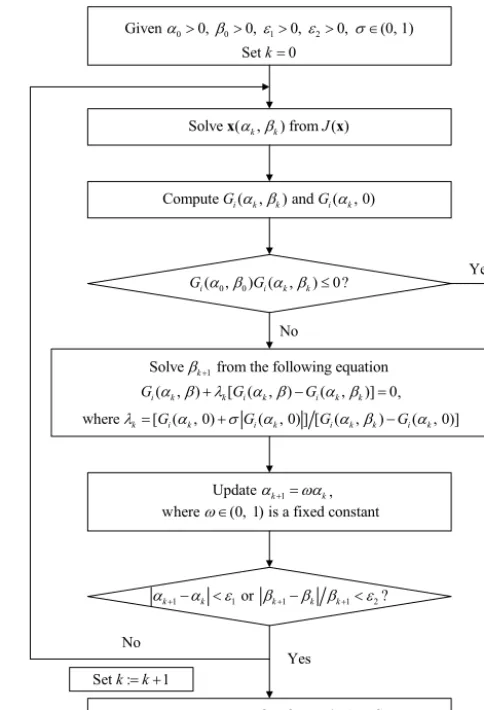
The flow chart of determining the regularization param-eters is shown in Fig. 2. For certain αk and βk, the

corresponding electron density Gi(αk, βk) and Gi(αk,0)

can be derived. If Gi(α0, β0)Gi(αk, βk)≤0, these αk and

βk are determined regularization parameters; otherwise,

βk+1 can be solved from the relaxation discrepancy

equa-tionGˆi(αk, β):=Gi(αk, β)+λk[Gi(αk, β)−Gi(αk, βk)] =

0, where λk=G_Gi(αk,0)+ ˆσ|Gi(αk,0)|

i(αk,βk)−Gi(αk,0) , and αk+1 can be

ob-tained by αk+1=ωαk, where ω∈(0,1) is a fixed

con-stant. When the iteration stop criterion, |_αk+1−αk|< ε1or

|_βk+1−βk|βk+1< ε2, whereε1andε2are constants, is

sat-isfied, the derived αk+1 and βk+1 are the optimal

regular-ization parameters, and the corresponding x is the recon-structed electron density; otherwise, theαk+1 andβk+1 are

set as the initial values to repeat the above steps. In the fol-lowing test, we takeγ=6.5,κ=3.5,ε1=10−5,ε2=10−8,

andω=0.618.

3 Results 3.1 Ideal test

In the ideal test, the real position between GNSS satellites and ground receivers on 8 March 2013 is used to establish the observation matrixA. The background electron density and simulated true electron density are both provided by the IRI2012 model (Bilitza et al., 2014). In this model, the IG (ionospheric global) index influences the electron density peak height, and the Rz (sunspot number) index influences the electron density peak density. To make the background electron density have a large difference from the simulated

Figure 2.The flow chart of determining the regularization parame-ters by using the linear model function method.

true electron density, the input parameters for the background model are set to IG−20, Rz−20 (denoting background I) and IG+20, Rz+20 (denoting background II). The simulated TEC measurement is derived by the length of the satellite-receiver ray propagating through each grid multiplied by the corresponding electron density (i.e., forward problem). To avoid the “inverse crime” and yielding unrealistically opti-mistic results, the grid sizes in the forward and inverse prob-lem are not the same (Kaipio and Somerrsalo, 2005). The spatial steps in the forward problem are 0.5◦in latitude, 0.5◦ in longitude, and 20 km in altitude. Due to the fact that the real measurements are inevitably subject to observational er-rors, noises are artificially imposed on the simulated TEC observations.

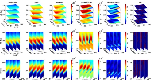
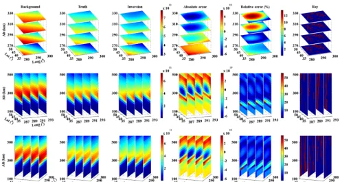
longi-Figure 3.The reconstruction results using regularization method I under background I conditions. From top to bottom are the longitude– latitude slices at different altitudes, altitude–latitude slices at different longitudes, and longitude–altitude slices at different latitudes. From left to right are the background electron density, true electron density, reconstructed electron density, reconstructed absolute error, reconstructed relative error, and whether the satellite-receiver ray propagates through the corresponding grid or not.

00:006 06:00 12:00 18:00

8 10 12 14 16 18 20 22 24

Hour (UT)

%

Background mean relative error SD of background relative error Inversion mean relative error SD of inversion relative error

Figure 4.The average relative reconstruction error and standard de-viation using regularization method I under the background I situ-ation. The red solid line is the average relative error of the back-ground electron density. The blue solid line is the standard deviation of the background relative error. The red dashed line is the average relative error of the reconstructed electron density. The blue dashed line is the standard deviation of reconstructed relative error.

tudes (287◦E, 289◦E, 291◦E, and 293◦E), and the altitude– longitude slices at different latitudes (39◦N, 41◦N, 43◦N, and 45◦N). From left to right are the background electron density, true electron density, reconstructed electron den-sity, reconstructed absolute error, reconstructed relative error, and whether the satellite-receiver ray propagating through the corresponding grid or not. The regularization parameters are 0.0146 and 0.1595, and the maximum absolute error of the reconstructed electron density is 1.5×1011electrons m−3

and mainly occurs near the southeast boundary of the recon-struction area. The maximum relative error is 96.48 %, and the large relative error mainly occurs at the height of about 170 km in the center and northwest of the reconstruction area. The average relative error is 12.89 %, and the standard devi-ation of the relative error is 8.61 %. Even though there are many satellite-receiver rays propagating through the certain grid, its reconstructed relative error is still large under some situations. The TEC measurement error caused by the differ-ent grid sizes in the forward and inverse problem are not the same along different satellite-receiver ray paths, leading to the large relative error in this region.

Figure 5.The reconstruction results using regularization method I under background II conditions. From top to bottom are the longitude– latitude slices at different altitudes, altitude–latitude slices at different longitudes, and longitude–altitude slices at different latitudes. From left to right are the background electron density, true electron density, reconstructed electron density, reconstructed absolute error, reconstructed relative error, and whether the satellite-receiver ray propagates through the corresponding grid or not.

8 10 12 14 16 18 20 22 24 26 28

%

Background mean relative error SD of background relative error Inversion mean relative error SD of inversion relative error

00:00 06:00 12:00 18:00

Hour (UT)

Figure 6.The average relative reconstruction error and standard de-viation using regularization method I under the background II sit-uation. The red solid line is the average relative error of the back-ground electron density. The blue solid line is the standard deviation of the background relative error. The red dashed line is the average relative error of the reconstructed electron density. The blue dashed line is the standard deviation of the reconstructed relative error.

background relative error (blue solid line) are also superim-posed for reference. After using the regularization method I, the average relative reconstruction error is significantly reduced compared with that of the background model, but the standard deviation of the relative reconstruction error in-creases during some periods.

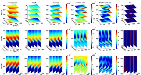
Figure 7.The reconstruction results using regularization method II under background I conditions. From top to bottom are the latitude-longitude slices at different altitudes, altitude–latitude slices at different latitude-longitudes, and latitude-longitude–altitude slices at different latitude-longitudes. From left to right are the background electron density, true electron density, reconstructed electron density, reconstructed absolute error, reconstructed relative error, and whether the satellite-receiver ray propagates through the corresponding grid or not.

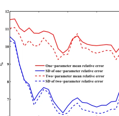
6 7 8 9 10 11 12

% _{One−parameter mean relative error}

SD of one−parameter relative error Two−parameter mean relative error SD of two−parameter relative error

00:00 06:00 12:00 18:00 Hour (UT)

Figure 8.The comparisons between the average relative error and standard deviation of the reconstructed relative error using regular-ization method II and the average relative error and standard devi-ation of the relative error using the single-parameter regularizdevi-ation method under background I conditions.

background electron density is lower than the simulated true electron density. The regularization parameters are 0.0012 and 5×10−5, and the maximum absolute error of the recon-structed electron density is about 5×1010electrons m−3and mainly occurs near the center of the reconstruction area. The maximum relative error is 115.07 %, the large relative error mainly occurs at the height of about 170 km in the center and north of the reconstruction area, the average relative recon-struction error is 11.04 %, and the standard deviation of the reconstructed relative error is 10.33 %.

Figure 8 shows the average relative error of the recon-structed electron density (red dashed line) and standard de-viation of the reconstructed relative error (blue dashed line) on 8 March. For comparison, the average relative error (red solid line) and standard deviation of the relative error (blue solid line) using the single-parameter regularization method are also shown. The cost functional of the single-parameter regularization method should be minimized to derive the ap-proximate solution of the ionospheric electron density:

J (x)=1

2(Ax−y)

T_R−1_(Ax−y)+α

2(x−xb)

T

B−1(x−xb)=min, (9)

Figure 9.The reconstruction results using regularization method II under background II conditions. From top to bottom are the longitude– latitude slices at different altitudes, altitude–latitude slices at different longitudes, and longitude–altitude slices at different latitudes. From left to right are the background electron density, true electron density, reconstructed electron density, reconstructed absolute error, reconstructed relative error, and whether the satellite-receiver ray propagates through the corresponding grid or not.

7 8 9 10 11 12 13

%

One−parameter mean relative error SD of one−parameter relative error Two−parameter mean relative error SD of two−parameter relative error

00:00 06:00 12:00 18:00

Hour (UT)

Figure 10.The comparisons between the average relative error and standard deviation of the relative error using regularization method II and the average relative error and standard deviation of the rel-ative error using the single-parameter regularization method under background II conditions.

in the vertical and horizontal direction, respectively, and the correlation distances are taken from Yue et al. (2007a). The average relative error and standard deviation of the recon-structed electron density using the dual-parameter regulariza-tion method are generally smaller than those of using single-parameter regularization method.

Figure 9 is the same as Fig. 7, but for the reconstruction results under the background II conditions. The regulariza-tion parameters are 0.0012 and 5.14×10−4, and the max-imum absolute error of the reconstructed electron density is about 6×1010electrons m−3and mainly occurs near the cen-ter of the reconstruction area. The maximum relative error is 55.32 %, the large relative error occurs mainly at the height of about 170 km in the center and northwest of the recon-struction area, the average relative error is 12.21 %, and the standard deviation of relative error is 8.93 %. Figure 10 is the same as Fig. 8, but for the reconstruction results under the background II condition, the reconstructed electron density using the dual-parameter regularization method show further improvement compared with that using the single-parameter regularization method.

0 2 4 6 100

300

500 00:00 UT

0 1 2 3 4 5 100

300

500 01:00 UT

0 1 2 3 4

100 300

500 02:00 UT

0 1 2 3

100 300

500 03:00 UT

0 1 2 3

100 300

500 04:00 UT

0 1 2 3

100 300

500 05:00 UT

0 1 2 3

100 300

500 06:00 UT

Alt (km)

0 1 2 3

100 300

500 07:00 UT

0 1 2

100 300

500 08:00 UT

0 0.5 1 1.5 2 100

300

500 09:00 UT

0 1 2 3

100 300

500 10:00 UT

0 1 2 3 4

100 300

500 11:00 UT

0 1 2 3 4 5 100

300

500 12:00 UT

0 2 4 6

100 300

500 13:00 UT

0 2 4 6 8

100 300

500 14:00 UT

0 6

100 300

500 15:00 UT

0 5 10

100 300

500 16:00 UT

0 5 10

100 300

500 17:00 UT

0 5 10

100 300

500 18:00 UT

0 5 10

100 300

500 19:00 UT

0 5 10

100 300

500 20:00 UT

Electron density (10 m )11 -3

0 5 10

100 300

500 21:00 UT

0 5 10

100 300

500 22:00 UT

0 2 4 6

100 300

500 23:00 UT Inversion Background Ionosonde measurement

Figure 11.The comparisons between the reconstructed electron density profiles near the MHJ station and the measured electron density profiles from ground ionosonde under the relatively quiet geomagnetic activity condition; LT=UT−4.6 h.

Overall, when the observation data are sparse, the regular-ization method II has a better performance. In the following, only the reconstruction results using regularization method II are shown in the real measurements test.

3.2 Real observation

In the real measurements cases, the effectiveness of the reg-ularization method II is tested under the quiet and active ge-omagnetic activity conditions. The ionosonde measurement from MHJ station is used as the independent validation data. These data were obtained from GIRO and were manually scaled by the SAO software, and they can provide accurate electron peak density and peak height. Due to the topside ionospheric electron density profiles derived by the extrapo-lation method, the electron density data below the height of 500 km are used to validate the reconstruction result. In the real reconstruction, it is assumed that the electron density in each grid does not vary within a 15 min interval.

The geomagnetic activity on 8 March was relatively quiet. The reconstruction results are shown in Fig. 11, in which the red line is the reconstructed electron density profile, the blue line is the background electron density profile, and the green line is the observed electron density profile from ground ionosonde. There are no ionosonde data at 01:00 and 12:00 UT. Overall, the reconstructed peak electron

den-sity using the regularization method II is much closer to the ionosonde measurements compared with that from the back-ground model, and the reconstructed electron density peak height is basically similar to the background value. This is mainly because the satellite-receiver geometry has limi-tations, and the TEC data contain much more ionospheric structure information in the horizontal direction than in the vertical direction. Only GNSS TEC data have limited influ-ences on the changes in altitudinal resolution in the back-ground model.

0 2 4 6 100

300 500

0 2 4 6

100 300 500

0 2 4 6

100 300 500

0 1 2 3 4 5 100

300 500

0 1 2 3 4

100 300 500

0 1 2 3 4

100 300 500

0 1 2 3 4

100 300 500

Alt (km)

0 1 2 3

100 300 500

0 0.5 1 1.5 2 2.5 100

300 500

0 1 2

100 300 500

0 1 2 3

100 300 500

0 1 2 3 4

100 300 500

0 1 2 3 4 5 100

300 500

0 2 4 6

100 300 500

0 2 4 6 8

100 300 500

0 2 4 6 8

100 300 500

0 2 4 6 8

100 300 500

0 2 4 6 8

100 300 500

0 5 10

100 300 500

0 5 10

100 300 500

0 5 10 15

100 300 500

0 5 10

100 300 500

0 2 4 6 8

100 300 500

0 2 4 6

100 300 500 Inversion Background Ionosonde measurement

00:00 UT 01:00 UT 02:00 UT 03:00 UT 04:00 UT 05:00 UT

06:00 UT 07:00 UT 08:00 UT 09:00 UT 10:00 UT 11:00 UT

12:00 UT 13:00 UT 14:00 UT 15:00 UT 16:00 UT 17:00 UT

18:00 UT 19:00 UT 20:00 UT

Electron density (10 m )11 3

21:00 UT 22:00 UT 23:00 UT

-Figure 12.The comparisons between the reconstructed electron density profiles near the MHJ station and the measured electron density profiles from ground ionosonde under the relatively active geomagnetic activity condition; LT=UT−4.6 h.

and temporal variations of the measurement error also need some more researches.

4 Conclusions

Ionospheric tomography based on GNSS TEC is a typical ill-posed inverse problem, and the regularization method is used to solve this problem by incorporating prior constraints to approximate the real electron density distribution. Because of the complexity of the spatial and temporal variations of the ionosphere, a single regularization term may not obtain the high-accuracy reconstruction results. Multiple constraints sometimes need to be incorporated, and multiple regulariza-tion parameters are introduced accordingly. Here, the iono-spheric variations are separated in the horizontal and vertical direction. The cost functional of the dual-parameter regular-ization method is established, and the regularregular-ization param-eters are determined by the linear model function method. This regularization algorithm is tested by the ideal cases and real cases, and the results show that it can significantly im-prove the background model outputs. Moreover, to imim-prove the reconstruction accuracy further, the measurement error and the background error covariance should be studied in de-tail.

Data availability. The GNSS observation data and precise ephemeris data can be obtained from ftp://cddis.gsfc.nasa.gov/ pub/gps/data/daily/2013/067/13o/ through FlashFXP software, and the ionosondes data can be obtained from the Digital Ionogram DataBase (DIDBase) (http://umlcar.uml.edu/DIDBase/) through SAO Explorer after applying for a personal account (MHJ45 MILLSTONE HILL, September 2018).

Acknowledgements. The authors would like to thank the IGS for providing the observation data and precise ephemeris data, and GIRO for the ionosondes data. This research was supported by the National Natural Science Foundation of China (no. 41575026, and no. 41804149).

The topical editor, Keisuke Hosokawa, thanks Gopi Krishna Seemala and two anonymous referees for help in evaluating this paper.

References

Alizadeh, M. M., Schuh, H., Todorava, S., and Schmidt, M.: Global ionosphere maps of VTEC from GNSS, satellite al-timetry, formosat-3/COSMIC data, J. Geod., 85, 975–987, https://doi.org/10.1007/s00190-011-0449-z, 2011.

Austen, J. R., Franke, S. J., and Liu, C. H.: Ionospheric imaging using computerized tomography, Radio Sci., 23, 299–307, 1988. Bilitza, D., Altadill, D., Zhang, Y., Mertens, C., Truhlik, V., Richards, P., McKinnell, L.-A., and Reinisch, B.: The inter-national reference ionosphere 2012 – A model of interna-tional collaboration, J. Space Weather Space Clim., 4, 689–721, https://doi.org/10.1051/swsc/2014004, 2014.

Bust, G. S., Garner, T. W., and Gaussiran II, T. L.: Ionospheric data assimilation three-dimensional (IDA3D): A global, multisensory, electron density specification algorithm, J. Geophys. Res., 109, A11312, https://doi.org/10.1029/2003JA010234, 2004.

Chen, Z., Lu, Y., Xu, Y., and Yang, H.: Multi-parameter Tikhonov regularization for linear ill-posed operator equations, J. Comput. Math., 26, 37–55, 2008.

Dettmering, D., Schmidt, M., and Heinkelman, R.: Combi-nation of different space-geodetic observations for re-gional ionosphere modeling, J. Geod., 85, 989–998, https://doi.org/10.1007/s00190-010-0423-1, 2011.

Fehmers, G. C., Kamp, L. P. J., Sluijter, F. W., and Spoel-stra, T. A. T.: A model-independent algorithm for ionospheric tomography: 1. Theory and tests, Radio Sci., 33, 149–163, https://doi.org/10.1029/97RS03007, 1998.

Fougere, P. F.: Ionospheric radio tomography using maximum en-tropy: 1. Theory and simulation studies, Radio Sci., 30, 429–444, 1995.

Garcia, R. and Crespon, F.: Radio tomography of the iono-sphere: Analysis of an underdetermined, ill-posed inverse problem, regional application, Radio Sci., 43, RS2014, https://doi.org/10.1029/2007RS003714, 2008.

Golub, G. H., Heath, M., and Wahba, G.: Generalized cross-validation as a method for choosing a good ridge parameter, Technometrics, 21, 215–223, 1979.

Hajj, G. A., Ibanez-Meier, R., Kursinski, E. R., and Ro-man, L. J.: Imaging the ionosphere with the global posi-tioning system, Int. J. Imaging Syst. Technol., 5, 174–184, https://doi.org/10.1002/ima.1850050214, 1994.

Hansen, P. C. and O’Leary, D. P.: The use of the L-curve in the reg-ularization of discrete ill-posed problems, SIAM J. Sci. Comput., 14, 1487–1503, 1993.

Hobiger, T., Kondo, T., and Koyama, Y.: Constrained simultaneous algebraic reconstruction technique (C-SART) – a new and sim-ple algorithm applied to ionospheric tomography, Earth Planets Space, 60, 727–735, 2008.

Huang, S. X. and Wu, R. S.: Methods of Mathematical Physics in Atmosphere Science, 3rd edn., China Meteorological Press, Bei-jing, China, 2011.

Jin, R., Jin, S., and Feng, G.: M-DCB: Matlab code for estimating GNSS satellite and receiver differential code biases, GPS Solut., 16, 541–548, https://doi.org/10.1007/s10291-012-0279-3, 2012. Kaipio, J. and Somersalo, E.: Statistical and Computational Inverse

Problems, Springer, New York, 2005.

Kunisch, K.: On a class of damped Morozov principles, Computing, 50, 185–188, https://doi.org/10.1007/BF02243810, 1993. Lee, J. K., Kamalabadi, F., and Makela, J. J.: Localized

three-dimensional ionospheric tomography with GPS ground receiver measurements, Radio Sci., 42, RS4018, https://doi.org/10.1029/2006RS003543, 2007.

Ma, X. F., Maruyama, T., Ma, G., and Takeda, T.: Three-dimensional ionospheric tomography using

observa-tion data of GPS ground receivers and ionosonde by neutral network, J. Geophys. Res., 110, A05308, https://doi.org/10.1029/2004JA010797, 2005.

Mallows, C. L.: Some comments on Cp, Technometrics, 15, 661– 675, 1973.

Markkanen, M., Lehtinen, M., Nygrén, T., Pirttila, J., Helenius, P., Vilenius, E., Tereshchenko, E. D., and Khudukon, B. Z.: Bayesian approach to satellite radio tomography with applica-tions in the Scandinavian sector, Ann. Geophys., 13, 1277–1287, 1995.

Mitchell, C. N. and Spencer, P. S.: A three-dimensional time-dependent algorithm for ionospheric imaging using GPS, Ann. Geophys., 46, 687–696, 2003.

Na, H. and Lee, H.: Orthogonal decomposition technique for iono-spheric tomography, Int. J. Imaging Syst. Technol., 3, 354–365, 1991.

Norberg, J., Roininen, L., Vierinen, J., Amm, O., McKay-Bukowski, D., and Lehtinen, M.: Ionospheric to-mography in Bayesian framework with Gaussian Markov random field priors, Radio Sci., 50, 138–152, https://doi.org/10.1002/2014RS005431, 2015.

Nygrén, T., Markkanen, M., Lehtinen, M., Tereshchenko, E. D., and Khudukon, B. Z.: Stochastic inversion in iono-spheric radio tomography, Radio Sci., 32, 2359–2373, https://doi.org/10.1029/97RS02915, 1997.

Pi, X., Wang, C., Hajj, G. A., Rosen, G., Wilson, B. D., and Bailey, G. J.: Estimation of E×B drift using a global assimilative ionospheric model: An observation sys-tem simulation experiment, J. Geophys. Res., 108, 1075, https://doi.org/10.1029/2001JA009235, 2003.

Raymund, T. D., Austen, J. R., Franke, S. J., Liu, C. H., Klobuchar, J. A., and Stalker, J.: Application of computerized tomography to investigation of ionospheric structures, Radio Sci., 25, 771–789, 1990.

Schunk, R. W., Scherliess, L., Sojka, J. J., Thompson, D. C., An-derson, D. N., Codrescu, M., Minter, C., Fuller-Rowell, T. J., Heelis, R. A., Hairston, M., and Howe, B. M.: Global assim-ilation of ionospheric measurements (GAIM), Radio Sci., 39, RS1S02, https://doi.org/10.1029/2002RS002794, 2004. Seemala, G. K., Yamamoto, M., Saito, A., and Chen, C.-H.:

Three-dimensional GPS ionospheric tomography over Japan using con-strained least squares, J. Geophys. Res.-Space, 119, 3044–3052, https://doi.org/10.1002/2014RS005431, 2014.

Wang, C., Hajj, G., Pi, X., Rosen, I. G., and Wilson, B.: Develop-ment of the global assimilative ionospheric model, Radio Sci., 39, RS1S06, https://doi.org/10.1029/2002RS002854, 2004. Wang, Z.: Multi-parameter Tikhonov regularization and model

function approach to the damped Morozov principle for choosing regularization parameters, J. Comput. Appl. Math., 236, 1815– 1832, 2012.

Wen, D. B., Wang, Y., and Norman, R.: A new two-step algorithm for ionospheric tomography solution, GPS Solut., 16, 89–94, https://doi.org/10.1007/s10291-011-0211-2, 2012.

us-ing GPS and Incoherent Scatter Radar observations, Ann. Geo-phys., 25, 1815–1825, https://doi.org/10.5194/angeo-25-1815-2007, 2007a.

Yue, X., Wan, W., Liu, L., Zheng, F., Lei, J., Zhao, B., Xu, G., Zhang, S.-R., and Zhu, J.: Data assimilation of incoherent scat-ter radar observation into a one-dimensional midlatitude iono-spheric model by applying ensemble Kalman filter, Radio Sci., 42, RS6006, https://doi.org/10.1029/2007RS003631, 2007b.